Jacques F´ejoz
1, Andreas Knauf
2, Richard Montgomery
31
Universit´e Paris-Dauphine & Observatoire de Paris, [email protected]
2
Department of Mathematics, Friedrich-Alexander-University Erlangen-N¨urnberg, Cauerstr. 11, D-91058 Erlangen, Germany, [email protected]
3
Mathematics Department, UC Santa Cruz, 4111 McHenry, Santa Cruz, CA 95064, USA, [email protected]
June 7, 2016
Abstract. Motivated by the high-energy limit of the N -body problem we construct non-deterministic billiard process. The billiard table is the comple-ment of a finite collection of linear subspaces within a Euclidean vector space. A trajectory is a constant speed polygonal curve with vertices on the subspaces and change of direction upon hitting a subspace governed by “conservation of momentum” (mirror reflection). The itinerary of a trajectory is the list of sub-spaces it hits, in order. (A) Are itineraries finite? (B) What is the structure of the space of all trajectories having a fixed itinerary? In a beautiful series of papers Burago-Ferleger-Kononenko [BFK] answered (A) affirmatively by us-ing non-smooth metric geometry ideas and the notion of a Hadamard space. We answer (B) by proving that this space of trajectories is diffeomorphic to a Lagrangian relation on the space of lines in the Euclidean space. Our methods combine those of BFK with the notion of a generating family for a Lagrangian relation.
1. Introduction. .
1.1. Euclidean Data. Point Billiards. Motivating Example. Consider a Euclidean vector space E endowed with a finite collection L of linear subspaces which we call “collision subspaces”. Write
(1) C= ⋃
L∈L
L (collision locus) for the collision locus and
(2) E0= E ∖ C (our billiard table)
for its complement. Play billiards on E0 !
A “billiard trajectory” will be a certain type of polygonal curve q∶ R → E all of whose vertices are collisions, i.e. lie on C. When q hits a subspace L∈ L it switches directions by bouncing off of L according to the laws of reflection (see equations (4), (5) below). Imagine light rays bouncing off of a finite collection of reflective wires (lines) in E= R3
.
1
1.1.1. Motivating Example: N -body billiards. E= (Rd)N is the configuration space for the N massive point particles moving in d–dimensional Euclidean space Rd. Endow E with its mass metric, by which we mean the inner product whose squared norm is twice the kinetic energy. Take L to consist of the (N
2) binary collision subspaces
(3) ∆ab= {q = (q1, . . . , qN), qi∈ Rd∶ qa= qb} ⊂ E for some pair a≠ b.
We call this class of examples “N -body billiards”. See the next section for details. 1.1.2. Billiard Rules. We now define what it means for a polygonal curve q∶ R → E to be a billiard trajectory. By a collision point for q we mean a time t or the corresponding point q(t) such that q(t) ∈ C. Thus at a collision point q(t) ∈ L for some L∈ L. We assume that collision points are discrete. In particular no edge of q lies within an L. Every vertex of q is a collision point. The velocities v−, v+ of q immediately before and after collision with L∈ L are well-defined and locally constant. They suffer a jump v−↦ v+ at collision. Let
πL∶ E → L
be orthogonal projection onto L. We require each velocity jump to obey the rules: (4) ∥v−∥ = ∥v+∥ “conservation of energy”
(5) πL(v+) = πL(v−) “conservation of momentum”
In N-body billiards (1.1.1) these rules correspond to conservation of energy and momentum. (Note that the rules allow for no jump: v−= v+.)
To summarize, a billiard trajectory for(E, ⟨⋅, ⋅⟩, L) is an oriented polygonal curve in E with vertices on collision subspaces, and no edge of which lies within a collision subspace. At each collision the velocity jump v−→ v+ obeys the two rules (4, 5) above. Without loss of generality we will assume the curve’s speed is 1.
1.1.3. Multiple collisions. The attentive reader will have noticed that the law of reflection (5) is ambiguous if the collision point q∗ belongs to more than one L. This ambiguity is analogous to the problem of trying to define standard billiard dynamics at the corner pocket of a polygonal billiard table in the plane. We get around this ambiguity by agreeing to choose one of the collision subspaces to which q∗ belongs and then using only that subspace in implementing law (5). Thus we view billiard trajectories with multiple collisions as coming with the extra structure of a labelling of collision points, with each collision point being labelled by one of the L∈ L to which it belongs. For more on problems arising with multiple collisions see subsection2.1further on.
1.1.4. Dimension and Transversality. For simplicity of exposition we will hence-forth assume that each subspace L has the same codimension d and d≥ 1. This assumption excludes various pathologies such as L1 ⊂ L2 occuring within our col-lectionL of subspaces.
In addition to being all of the same codimension d, the collection (eq (3)) of collision subspaces for N-body billiards are pairwise transversal: codim(L1∩ L2)= 2d for all distinct pairs L1, L2∈ L. We believe such transversality assumptions may be very useful in future work.
1.1.5. Non-deterministic Dynamics. For a given incoming v− ∈ E ∖ 0 to a q∗ ∈ L there is a(d−1)–dimensional sphere’s worth of choices for the outgoing v+’s, namely the set of all solutions to eq (4, 5) for that fixed v−. It follows that the billiard process is non-deterministic: there is no univalued rule that takes us from the past motion to the future motion. However, we do not view our billiard dynamics as a stochastic process. Rather we think of our billiard trajectories as arising as limits of deterministic N -body dynamics, and we are interested in what is the set of all possible limits. See section2 below.
(Even if d= 1 we do not have deterministic dynamics, since the 0-sphere consists of two choices. It is standard to turn this case into a deterministic dynamics by requiring transversality: v+≠ v−at each collision. This is what is done for N point particles moving on the line: the dynamics preserves their order on the line. The game is equivalent to playing billiards on a closed polyhedral cone in RN.) 1.2. Basic Questions and Main result.
1.2.1. Fundamental Finiteness Theorem.
QUESTION 1. Is the total number of collisions of a billiard trajectory finite? The answer is the fundamental theorem of the subject.
Background Theorem 1 ([BFK1, BFK2]). There is a K = K(E, ⟨⋅, ⋅⟩, L) such that every trajectory has less than or equal to K collisions.
To appreciate the subtlety of the problem of computing the smallest K, even in apparently simple deterministic (d= 1) situations, we strongly urge the reader to take a peek at [Gal].
1.2.2. Itineraries.
Definition 1. The itinerary of a billiard trajectory is the list of collision subspaces L∈ L that it intersects, in their order of occurrence.
By the Background Theorem of BFK just stated, any realized itinerary has length less than or equal to K. So if there are a total of M subspaces in L, then the set of all realized itineraries is a finite set of length less than MK. (Repeats such as L1L1. . .are not allowed, hence the strict inequality.)
QUESTION 2. What is the finite set of all itineraries which are realized by some billiard trajectory?
This is a hard question about which we have very little to say.
We can observe that beyond Li+1 ≠ Li there may be other ‘topological’ re-strictions on the allowable itineraries. For example, for N ≥ 4 bodies on the line (d= 1; E = RN) after the itinerary(∆12,∆34,∆23) particles 1 and 4 can no longer be neighbors, whether or not collisions change the ordering (are transverse). So (∆12,∆34,∆23,∆14) cannot be realized.
In section8.1we give some partial results regarding this question when each L is a line.
1.2.3. Space of trajectories realizing a given itinerary. Suppose a particular itinerary is realized. We can then ask about all of its realizations.
QUESTION 3. What is the structure (dimension, smoothness, symplectic char-acter) of the space of all billiard trajectories having a given itinerary?
Answering Question 3 is the point of our paper.
From now on we fix an itinerary L1L2. . . Lk, with Li∈ L.
Defining the space B of point billiard trajectories realizing the itinerary. Write B(L1. . . Lk), or simply B for the space of all billiard trajectories realizing the given itinerary. Let us be more precise: a billiard trajectory q is in the subsetB(L1. . . Lk) if and only if there are exactly k distinct collision times:
(6) t1< t2< . . . tk, q(ti) ∶= qi∈ Li. We emphasize that
(7) qi≠ qi+1, i= 1, 2, . . . , k − 1
since ∣qi+1− qi∣ = ti+1− ti > 0. Also qi+1− qi, qi− qi−1 ∉ Li since no edge of q lies in the collision locus. Condition (7) does not exclude the possibility of qi∈ L′ for some L′∈ L, L′≠ Li, Li+1, Li−1. In this case we label qi with L= Li when applying our ‘conservation of momentum” rule eq (5). We endowB with the compact-open topology.
A trajectory q ∈ B(L1. . . Lk) has an initial ray r− parameterized by the initial segment(−∞, t1) where q1= q(t1) is the first collision. Similarly q has a final ray r+parameterized by the final segment(tk,∞) where qk= q(tk) is the final collision along q. Extend the rays to oriented lines ℓ−, ℓ+. We want to think of the fixing of the itinerary as defining a “scattering map”
(8) ℓ+↦ ℓ+
on the space LINES(E) of oriented lines in E. (We will elucidate the structure of LINES(E) as a symplectic manifold momentarily.) However, this “scattering map” is almost never a map in that one ℓ− may give rise to many ℓ+’s. See example 1 below. Instead we have “scattering relation”
R = R(L1. . . Lk) ⊂ LINES(E) × LINES(E).
Definition 2. The scattering relationR = R(L1L2. . . Lk) associated to the chosen itinerary L1L2. . . Lk consists of all pairs(ℓ−, ℓ+) of incoming and outgoing lines for billiard trajectories q∈ B(L1. . . Lk).
We have just defined a continuous map
B → R ⊂ LINES(E) × LINES(E)
which sends each trajectory q∈ B(L1. . . Lk) to its incoming and outgoing (oriented) lines. The image of this map is the scattering relation. The group of time transla-tions acts on the space of billiard trajectories, sending q(t) to q(t − t0), for t0∈ R, without altering the itinerary or the incoming or outgoing line. Thus our map into the scattering relation induces a map on the quotient domain with the same image. We name this map the scattering projection.
(9) SCAT∶ B/R Ð→ R ⊂ LINES(E) × LINES(E) We can now state our main result.
Theorem 1. The scattering relationR is a Lagrangian relation on the symplectic manifold LINES(E) of oriented lines in E. In particular R is a smooth manifold of dimension 2(dim(E)−1). The scattering projection (eq (9)) defines a diffeomor-phism betweenB/R and R. In particular, modulo time translation, a point billiard
trajectory realizing the given itinerary is uniquely determined by its incoming and outgoing lines.
For completeness, we recall for the reader the definition of “Lagrangian relation” and the symplectic structure on LINES(E) in what immediately follows.
1.2.4. Lagrangian relations.
Definition 3. A Lagrangian relation on a symplectic manifold (P, ω) is a La-grangian submanifoldR of the product symplectic manifold ¯P × P, where the bar of “ ¯P” means we endow the product with the symplectic structure −ω ⊕ ω.
Graphs of symplectic maps P → P are Lagrangian relations. We think of La-grangian relations as generalized symplectic maps, that is, symplectic maps which are “allowed to go vertical” at various places.
1.2.5. The symplectic structure on the space of lines. An oriented line ℓ∈ LINES(E) can be represented by an initial position A∈ E and an initial velocity vA∈ Ev≅ E. (We use the subscript v in “Ev” to keep track of who is a velocity and who is a position.) The line associated to (A, vA) is parameterized as A + tvA. We will insist that velocities vA are unit: ∣vA∣ = 1. (A, vA) and (C, vC) represent the same oriented line if and only if vA= vC and C= A + svA for some real number s. There is a unique point Q ∈ ℓ closest to the origin of E. This Q is determined by the algebraic condition ⟨Q, vA⟩ = 0. Choosing Q as the initial position A on ℓ sets up a diffeomorphism between the space LINES(E) of oriented lines in E and the tangent bundle of the unit sphere in E:
LINES(E) ≅ TS(Ev) = {(v, Q) ∈ Ev× E ∶∣v∣ = 1, Q ⊥ v}.
Use the Euclidean structure to identify T S(Ev) with T∗S(Ev), thereby giving the space of lines a symplectic structure.
Remark. The diffeomorphism LINES(E) → TS(Ev) reverses the role of posi-tions and velocities. The position v∈ S(Ev) at which the tangent vector (v, Q) is attached represents the velocity vector v= vA of the corresponding line, while the tangent or Q-part of(v, Q) represents an initial position point on the line ℓ, namely the closest point to 0.
1.2.6. Lines as a reduced space. The space of oriented lines can be recast as a symplectic reduced space. Let H(A, v) = 1
2∣v∣ 2
be the usual Hamiltonian for free particle motion. Here(A, v) ∈ E ×Ev≅ E ×E∗≅ T∗E. The flow of the Hamiltonian vector field for H is φt(A, vA) = (A+tvA, vA) which is a symplectic R action on the full phase space. Its integral curves are lines. The level set H−1(1/2) consists of those initial conditions(A, v) such that ∣v∣ = 1. The space LINES(E) of oriented lines is thus the sub-quotient H−1(1/2)/R of E × E
v by this R action. This sub-quotient construction is precisely the symplectic reduction construction: LINES(E) with its symplectic structure is an instance of the construction of the “symplectic reduced space”. Write
(10) π∶ E × S(Ev) → LINES(E)
for the corresponding quotient map. Thus π(A, v) = π( ˜A,v˜) if and only if ˜v = v and ˜
1.2.7. The unreduced scattering relation. In order to prove and to better understand our main theorem 1 we must “unreduce” the relationR by working directly with normalized initial conditions(A, vA) ∈ E ×S(Ev) instead of the associated oriented line π(A, v) = ℓ. If q(t) is a billiard trajectory in B(L1. . . Lk) consider again its initial ray r−⊂ ℓ− and final ray r+⊂ ℓ+. Pick corresponding points A∈ r−, B ∈ r+ and the corresponding directions vA, vB. We emphasize that we are saying nothing about the times tA, tB at which the points A, B are selected along q(t). In this way we have chosen pairs(A, vA), (B, vB) ∈ E × Ev. The unreduced statement of theorem1 is
Theorem 2. For each q∈ B consider the two-parameter family of pairs of boundary conditions
((A, vA), (B, vB)) = ((q(t0), ˙q(t0)), (q(tk+1), ˙q(tk+1)))
lying on the incoming and outgoing rays of q. (Here t0 < t1 and tk+1 > tk as per eq (6).) As q varies over B these pairs sweep out a Lagrangian relation ˜R =
˜
R(L1. . . Lk) on E × Ev. The projection ((A, vA), (B, vB)) ↦ (A, B) maps ˜R dif-feomorphically onto an open subset of E× E. The projection of ˜R to LINES(E) × LINES(E) by π × π (where π is as in eq10) is the relationR of theorem1. Remark on algebraicity. Our Lagrangian relations are semi-algebraic varieties: they are defined by algebraic equations together with algebraic inequalities. This fact follows from our proof of the theorem using generating functions.
Remark: Scaling, Symmetries and Conservation Laws. Point billiard trajectories enjoy a scaling symmetry. N -body billiards enjoy translational and rotational symmetries and the consequent conserved quantities of linear and angular momentum. Details of these symmetries are discussed in section7.
2. Motivation : The Gravitational N –Body Problem.
We go into some detail regarding our underlying motivation. The basic set-up, E = (Rd)N with the collision subspaces being the binary collision subspaces ∆ab was described above in subsection1.1.1and we keep the same notation.
Positive energy solutions to the gravitational two-body problem, viewed in a center-of-mass frame, consist of a pair of coplanar hyperbolas sharing the origin as a focus. Viewed from afar away, these hyperbolas become indistinguishable from their asymptotes: the two bodies come in along their separate rays, bounce off each other, to head back to infinity along different rays.
For the gravitational N -body problem the same space-time picture holds when viewed from away from all close encounters. Each body moves nearly on a straight line at nearly constant speed until it comes into very close vicinity of another body at which time it veers off to recede along another near-line at near-constant speed. In the limit 1
, what happens at these close encounters is the bodies “bounce off” each other. The direction of this “bouncing” will look random unless we know detailed specifics of the incoming motion. Without these details, all we can say is that each bounce is an elastic collision : total energy and linear momentum are conserved. These two conservation laws are encoded by our rules of reflection (eq (4,5).
1
Thus we expect certain families of positive energy solutions to the graviational N-body problem will limit onto N -body billiard trajectories as described above (see subsection1.1.1). In a subsequent paper we will prove this assertion by showing that N-body billiard trajectories are “shadowed” by families of trajectories of positive energy solutions to the gravitational N -body problem.
2.1. Multiple Collisions and clusters. A collision between three or more parti-cles (or two or more simultaneous binary collisions) corresponds to a point q∈ (Rd)N lying in several ∆ab. The paper of Mather and McGehee [McG], and subsequent work on non-collision singularities based on their ideas make suspect the validity of our underlying assumption (4) of conservation of kinetic energy when trying to model such multiple collision events with point billiards. Mather and McGehee establish the existence of a set of initial conditions for 4 bodies (on the line) where the kinetic energy starts out O(1) and in a finite time becomes arbitrarily large, arbitrarily far away from the close encounter region. The infinite negative potential energy well of near-triple collision serves as a source which one of the bodies can extract to make its speed arbitrarily high. We imagine the following caricature of celestial mechanics based on the notion of cluster decompositions [DG], where each clusters represents a subset of close tightly bound particles. Total energy and mo-mentum is preserved for each isolated cluster. But not all energy need be kinetic. We could even allow trajectories to move inside intersections of the ∆ab, corre-sponding to systems that are bound over some large interval of time. At collisions between clusters, corresponding groups of particles can experience inelastic scatter-ing, potential energy being stored in groups or released from it, and redistributed.
3. Generating Families and the proof.
The chord length between successive impacts of the ball with the table serves as the generating function for the standard billiard map associated to a convex table in the plane. So it is not a great surprise that the path length of finite segments of polygonal paths realizing the given itinerary serves a similar function for our non-deterministic billiard processes. Fix points A= q0on the incoming ray and B= qk+1 on the outgoing ray of the billiard trajectory q∈ B. Let qi∈ Libe the intermediate collision points as per eq (6). Then the length of the segment q([t0, tk+1]) is: (11) S(A, q1, . . . , qk, B)= ∣A − q1∣+ ∣q1− q2∣+ . . . + ∣qk−1− qk∣+ ∣qk− B∣
and this is also the travel time of this segment. We turn this observation around to find the billiard trajectories as critical points of S.
Minimization Problem.
Fix A, B∈ E ∖ C. Minimize (11) over all intermediate choices qi∈ Li.
Write xy for the line segment joining x to y, x, y∈ E, parameterizing xy so as to have unit speed. If xi ∈ E are a collection of points then by x1x2x3. . . xn we will mean the polygonal path with n− 1 edges xixi+1. Let
Λ= L1× L2× . . . × Lk.
Then if A, B ∈ E and λ = (q1, . . . , qk)∈ Λ we write AλB for the piecewise linear segment Aq1q2. . . qkB.
Definition 4. We will say that λ∈ Λ is “generic” if q1 ∉ L2, qk ∉ Lk−1 and qi ∉ Li−1∪ Li+1,1< i < k.
We will say that(A, λ, B) ∈ E × Λ × E is ‘generic” if λ is generic, if A, B ∈ E0 and if the rays qiAand qkB have no collisions besides their initial points q1, qk. We will call the open set of all generic points in E× Λ × E the “generic set”.
Define
(12) SA,B∶ Λ → R; SA,B(q1, q2, . . . , qk) = S(A, q1, q2, . . . , qk, B)
by viewing the action (11) to be a function of the intermediate intersection points qi alone, with A, B∈ E as parameters.
Proposition 1. Suppose(A, λ, B) is generic in the sense of definition4. Then the following are equivalent.
● (A) λ is a critical point of SA,B
● (B) AλB is a segment of a billiard trajectory realizing the given itinerary. If either condition holds then the direction of the incoming line of the associated billiard trajectory is vA= −∇AS(A, λ, B) while the direction of the outgoing line is vB= +∇BS(A, λ, B) where ∇AS,∇BS∶ E0× Λ × E0→ E denote the gradients with respect to the A, B variables.
Example 1. [Total Collision] Consider the caseL = {0}, so that the only subspace is the 0 subspace. A linear billiard trajectory realizing the itinerary (0) consists of an angle with vertex at 0. The parameter space Λ is the single point 0. The action is S(A, 0, B) = ∣A∣ + ∣B∣. The intermediate collision point q1 = 0 cannot be varied so the condition dλS = 0 is vacuous. We compute ∇AS = A/∣A∣, ∇BS = B/∣B∣ consequently the Lagrangian relation of theorem2consists of all quadruples ((A, vA), (B, vB)) ∈ TE × TE for which vA= −A/∣A∣ and vB= B/∣B∣, and A, B ≠ 0. The first pair(A, −A/∣A∣) represents the initial position and velocity of a line thru the origin, moving towards the origin. The final pair (B, B/∣B∣) represents the initial position and velocity for a line thru the origin moving away from the origin. Our incoming line and outgoing line both pass through the origin, so their “Q parts” are 0. (See subsubsection1.2.5.) Their v parts, vAand vBare arbitrary unit vectors. The Lagrangian relation R of theorem 1 is the product of the two zero sections of T∗S(E) = LINES(E).
Proposition 1 asserts that S is a “generating family” (also known as a “Morse family”) for the Lagrangian relation of theorem2. We recall the notion of a gener-ating family.
Definition 5. The function F ∶ E × Λ × E → R is a generating family for the Lagrangian relationR on E × Ev ifR consists of those quadruples (pairs of pairs) ((A, vA), (B, vB)) ∈ (E × Ev) × (E × Ev) for which there exists a λ ∈ Λ such that
● (i) (A, λ, B) is a smooth point of F, and
● (ii) dλF(A, λ, B) = 0, vA= −∇AF(A, λ, B) and vB= +∇BF(A, λ, B). Here ∇A,∇B are the gradients with respect to these first and last component vari-ables, A, B and dλF(A, λ, B) ∈ Λ∗ is the differential with respect to λ.
The notion of generating family was formalized by H¨ormander in [Hor1] [Hor2, Def. 25.4.3] under the name of “phase function”. Libermann and Marle [LiMa] use the name “Morse family” and we find their treatment exceptionally clear. (See Definition 1.10 in [LiMa, Appendix 7.1].) Paraphrasing: “Let π∶ B → N be a submersion and S∶ B → R be a differentiable function. The function S is called a Morse family (for N , or for R⊂ T∗N) if the image of the one-form dS∶ B → T∗B and the conormal bundle to the fibers of π, are transverse within T∗B. This transverse intersection is necessarily smooth and pushes down to T∗N where it forms a Lagrangian submanifold R, the Lagrangian submanifold for which S is the ‘Morse family’.”
The transversality condition in the definition just given of a Morse family is needed to insure that the corresponding Lagrangian submanifold is smooth. In our case we establish smoothness by establishing:
Proposition 2. Every critical point λ of SAB which is a generic point in the sense of definition4is a non-degenerate critical point, so transversality holds as discussed above. Indeed, the Hessian of SA,B at λ is positive definite.
3.1. Proof of proposition1. For the function x ↦∣x∣ we have that d∣x∣ = ⟨x,dx⟩∣x∣ . (The algebraic meaning of ‘dx’ here, as per computations found frequently in Chern or Cartan, is that dx is the identity map on E, this being the differential of the map x ↦ x. In other words, for v ∈ E (d∣x∣)(v) = ⟨x,v⟩
∣x∣ .) Similarly if x0 ∈ E is a constant vector then d∣x − x0∣ = ⟨x−x
0,dx⟩
∣x−x0∣ = ⟨n(x, x0), dx⟩, where we write
n(x, y) = x− y ∣x − y∣
for the unit vector pointing from y to x, assuming x ≠ y. Now write di for the differential of SA,B with respect to qi, keeping the other qj constant. We have
diSA,B= di(∣qi−1− qi∣ + ∣qi− qi+1∣) = ⟨n(qi, qi−1), dqi⟩ + ⟨n(qi, qi+1), dqi⟩. Since n(y, x) = −n(x, y), this yields
diSA,B= ⟨n(qi, qi−1) − n(qi+1, qi) , dqi⟩.
Now dqi is the identity on Li, so this differential is zero if and only if n(qi, qi−1) − n(qi+1, qi) ⊥ Li which is the same as requiring that πi(n(qi, qi−1) − n(qi+1, qi)) = 0, where we have written πifor πLi. But if the piecewise linear trajectory Aq1q2. . . qkB
is parametrized by arc length, traveling from A to B, then its velocity just be-fore collision with Li is vi,− = n(qi, qi−1) and its velocity just after collision is vi,+= n(qi+1, qi), so that our condition of criticality is equivalent to the condition of conservation of momentum (equation (5)) at collision i. Finally dSA,B= 0 if and only if for i= 1, 2, . . . , k we have diSA,B= 0. ◻
We postpone the proof of proposition2 to section5.
3.2. Proof of (most of ) theorem 2. Let q0∈ B(L1. . . Lk) with initial ray ℓin,0 and final ray ℓout,0. Let λ0= q0
1, q0 2, . . . , q0
k be its collision points. According to the definition of a billiard trajectory we cannot have qi+1∈ Li, 1≤ i ≤ k −1 for otherwise segment qiqi+1 ⊂ Li which is forbidden. Similarly qi−1∉ Li for 2≤ i ≤ k. Choose
points A0∈ ℓin,0, B0∈ ℓout,0. Then A0, B0∉ C. Thus (A0, λ0, B0) ∈ E × Λ × E is a generic point. And according to proposition1, λ0is a critical point of SA0,B0.
Now flip the logic around. Consider the map E× Λ × E → Λ∗ (13) (A, λ, B) z→ dSA,B(λ) ∈ Λ∗.
Proposition1 asserts that the zeros(A, λ, B) of this map which are generic points (in the sense of definition 4) are precisely the billiard segments for some q ∈ B(L1, L2, . . . , Lk).
The chosen segment of q0 from A0to B0is such a zero. We use Proposition2 in conjunction with the Implicit Function Theorem to get nearby, smoothly varying, zeros. The derivative of map (13) with respect to λ∈ Λ at A0λ0B0 is the Hessian of SA0,B0 with respect to λ, evaluated at λ0. Proposition 2 asserts this derivative
is invertible. The hypotheses of the Implicit Function Theorem hold. There exist neighborhoods U−⊂ E of A and U+⊂ E of B0and a smooth function U−× U+→ Λ, written(A, B) ↦ λ(A, B) such that Aλ(A, B)B is a zero of the map (13) and hence potentially part of a billiard segment lying inB. We complete this billiard segment to a full trajectory q∶ R → E by extending its initial and final segments Aq1and qkB to rays. We can guarantee that this extended full trajectory has no new collisions by taking a sufficiently small neighborhood U−, U+ of A0, B0 and recalling that the generic set is open. This full trajectory is now a billiard trajectory q∈ B with these q’s smoothly parameterized by their ‘endpoints” by(A, B) ∈ U−× U+.
We have just described billiards q∈ B as locally forming graphs over their ‘end-points’ (A, B). By direct computation the velocity of the initial ray at A is vA = (q1−A)/∣q1−A∣ = −∇ASwhile the velocity of final ray is vB= (B−qk)/∣B−qk∣ = ∇BS. Hence, when viewed in terms of initial and final conditions ((A, vA), (B, vB)) at points along initial and final rays, the space of billiard trajectories q∈ B is realized locally as a Lagrangian relation ˜R on E ×E which arises from the generating family S, and forms locally a graph over some open set in E0× E0
.
It remains to prove that these local graphs piece together to a global graph over an open dense subset of the space of endpoints E0× E0
. That ‘piecing to-gether’ is precisely the uniqueness assertion of the penultimate sentence of theorem 2which states that a billiard trajectory q∈ B is uniquely determined (modulo time translations) by its endpoints A, B. Proving this uniqueness requires a new tool, summarized in theorem3below.
The assertion of the last sentence of theorem 2 concerns the relation between the Lagrangian relation of theorem 2 and the relation described by theorem 1. The proof of this assertion is the same as the proof of theorem1 which now follows. ◻ 3.3. Proof of theorem1: Reducing Lagrangian Relations.
We will push the Lagrangian relation ˜R on E × Ev of theorem 2 down to a Lagrangian relation on LINES(E) and verify that it is the desired Lagrangian relationR.
Recall from subsubsection1.2.6that LINES(E) is the symplectic reduced space of E×Ev by the Hamiltonian flow for the free particle Hamiltonian H(q, v) = 12∣v∣
2 . As such LINES(E) is a subquotient of E × Ev with subquotient map written π ∶ H−1(1/2) → LINES(E). Observe that ˜R ⊂ H−1(1/2) × H−1(1/2), since whenever ((A, vA), (B, vB)) ∈ ˜R then vA, vBhave unit length. Regardless of what points A, B we pick along the initial ray ℓ−and final ray ℓ+of a fixed billiard trajectory q, we get
the same intermediate points λ= q1q2. . . qk. In other words,(A, vA; B, vB) ∈ ˜R and (A+hvA, vA; B+svB, vB) ∈ ˜R give rise to the same trajectory q, modulo translation (provided that h, s∈ R are appropriately restricted so we have not “passed” the first or last collision of the initial or final ray). In other words these different choices of A, B yield the same initial and final rays, and hence the same initial and final lines. But this action of (h, s) ∈ R × R generates precisely the kernel of the form −ω ⊕ω on (E ×Ev)×(E ×Ev) upon restricting this form to H−1(1/2)×H−1(1/2) ⊂ (E×Ev)×(E×Ev). It follows that ˜R ⊂ H−1(1/2)×H−1(1/2) descends by the quotient map π × π to yield our desired Lagrangian relationR ⊂ LINES(E)×LINES(E). ◻. 3.4. Uniqueness. What remains to do. We have established that our space B/R of billiard trajectories realizing the given itinerary, modulo time translation, is locally a graph over its initial and final rays. But theorem 2 and theorems 1 asserts thatB/R is globally a graph: there cannot be two billiard trajectories with the given itinerary which share the same initial and final rays. The uniqueness assertion will be established by proving:
Theorem 3. For A, B∈ E0
there is a unique global minimum λ∈ Λ for SA,B and no other critical points or local minima.
Caveat. The global minimizer λ∈ Λ of theorem3 might not yield a trajectory in B because it might suffer multiple collisions of the form qi = qi+1 which were explicitly excluded from being paths in B. See eq (7). Note that SAB fails to be smooth at such multiple collision points.
The proof of theorem3will be given in section4.
Finishing the proof of the main theorem 1, given theorem 3.
Let q∈ B be a billiard trajectory realizing the given itinerary. Choose a point A on its initial ray, B on its final ray, and let λ∈ Λ be the list of collision points ticked off the itinerary. By proposition1, λ is a critical point for SA,B. By theorem3, λ is the global minimum of SA,B and its only critical point. By proposition1 again, there are no other billiard trajectories which pass through A, tick off the given itinerary through a collision sequence, and then pass through B. In particular no other billiard trajectory shares q’s itinerary while having the same initial and final ray. This yields the uniqueness assertion of theorem1and the diffeomorphism assertion
of the penultimate sentence of theorem2. ◻
4. The Gluing of CATs. Proof of theorem 3.
We follow the non-smooth metric geometry ideas and construction in [BFK1] to obtain the proof of theorem3. (See also [BFK2].)
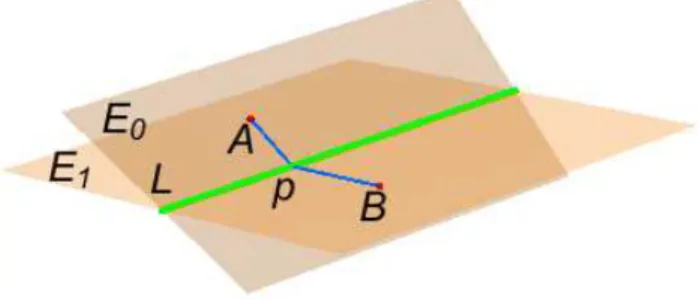
The main idea comes through clearly by looking into the case of a single subspace L = {L}, L ⊂ E, which is to say, an itinerary of length one. We form a new metric space EL by gluing two copies of E together along L. We call the two copies “sheets” and label them E0, E1. Thus
EL= E0∪LE1; Ei copies of E. See figure1 for the case where L is a line in the plane.
We define the metric on EL in terms of the minimizing geodesics between two points. If the two points lie in the same sheet then the geodesic between them is simply the usual line segment of E which joins them, viewed as lying in their shared
Figure 1. The metric space EL
sheet. If the two points A and B lie in different sheets, the only way we can travel from A to B is by passing through L to cross from one sheet to another. We are led to the problem of minimizing the distance from A to B, in E, among all paths which touch L in between. In other words, we must minimize SAB(p) = ∣A−p∣+∣p−B∣ over p∈ L. As we have seen, there is a unique minimizer p∗∈ L. Then the geodesic AB consists of the union of the line segment Ap∗ in A’s sheet and the segment p∗B in B’s sheet. The minimization problem is the same problem we encountered earlier. The geodesics in this case are in bijection with the point billiard trajectories having itinerary(L).
This construction of EL is a special case of a general metric gluing procedure which is the subject of a theorem by Reshetnyak. In order to describe Reshetnyak’s theorem we must recall what it means for a metric space to be “CAT(0)” and “Hadamard”.
Let (X, d) be a path-connected metric space. We define the length of a path in X by taking infimums of “polygonal approximations” to the path (see [BBI, Def. 2.3.1.]). X is called a length space if the distance d(A, B) between points A, B ∈ X is realized as the infimum of the lengths of paths between A and B. If X is also complete, then there is a shortest such path, denoted AB, and its length is d(A, B). We call AB a geodesic segment. (There may be more than one geodesic segment joining A and B.) A triangle ∆ABC in X is a subset consisting of three points A, B, C ∈ X together with geodesic segments AB, AC, BC joining them. A Euclidean comparison triangle ∆ ¯A ¯B ¯C⊂ R2for ∆ABC is a triangle in the Euclidean plane whose sides are congruent to those of ∆ABC: d(A, B) = ∥ ¯A− ¯B∥, d(A, C) = ∥ ¯A− ¯C∥ and d(A, C) = ∥ ¯B− ¯C∥. If x ∈ AB is a point on side AB, then there is a unique comparison point ¯x∈ ¯A ¯Bdefined by∥ ¯A−¯x∥ = d(A, x) , ∥¯x− ¯B∥ = d(x, B). Definition 6. [BBI, Defs. 4.1.9, 9.2.1.]) A CAT(0) space – also known as a space with non-positive curvature – is a complete length space (X, d) such that every sufficiently small triangle ∆ABC in X satisfies the following triangle comparison property. Let ∆ ¯A ¯B ¯C be a Euclidean comparison triangle for ∆ABC. If x∈ AB and ¯x∈ ¯A ¯B is the comparison point then d(x, C) ≤ ∥¯x − ¯C∥.
Definition 7. [BBI, Defs. 4.1.9, 9.2.1.] A Hadamard space is a simply-connected CAT(0) space.
The CAT(0) condition generalizes the Riemannian geometry condition that all sectional curvatures are non-positive to the case of (possibly) non-smooth metric
length spaces. The fiducial example of a Hadamard space is a Euclidean space. Hyperbolic space and metric trees are other examples.
Theorem 4. (Reshetnyak [BBI, 9.1.21.]) If X1 and X2 are Hadamard spaces containing isometric copies of the same convex set K, then the length space X1∪kX2 constructed by gluing X2 to X1 along K is again a Hadamard space.
Reshetnyak’s theorem asserts that the output of gluing Hadamard spaces serves as another input! We can iterate. If L1L2. . . Lk is an itinerary we thus form the Hadamard “itinerary” space
EL1L2...Lk= E0∪L1E1∪L2∪ . . . ∪LkEk.
Point billiard trajectories having itinerary L1L2. . . Lkyield geodesics which connect the first sheet E0 to the last sheet Ek.
Caveat. There may be minimizing geodesics in this Hadamard itinerary space which are not point billiard trajectories. These will be minimizers of SAB having either a multiple collision point qi= qi+1or an edge lying within an Li.
Proof of theorem 3. When X is Hadamard there is a unique geodesic AB joining any two points A, B∈ X. See, for example, Theorem 9.2.2 of [BBI]. ◻
5. The Hessian Proof of Proposition 2.
We continue with the same notation used in the proof of Proposition1 as above (subsection3.1), except now we add the shorthand:
(14) ni,j= n(qi, qj) ; ri,j= ∣qi− qj∣. Write d2
f for the Hessian of a function. Returning to the function ∣x∣ on E, a routine computation shows that
d2r=1
r∣dx − ⟨n, dx⟩n∣ 2
; n= x/r. An application of the chain rule now shows that
d2r12= 1
r12∣(dq1− dq2) − ⟨n12,(dq1− dq2)⟩n12∣ 2
which simply means that (d2 r12)(q1,q2)(ξ1, ξ2) = 1 r12∣(ξ1− ξ2) − ⟨n12,(ξ1− ξ2)⟩n12∣ 2 as a quadratic form on E× E. It follows that d2SA,B= k ∑ i=0 1
ri,i+1∣(dqi− dqi+1) − ⟨(dqi− dqi+1), ni,i+1⟩ni,i+1∣ 2
, provided we set q0= A, qk+1= B, dq0= 0, dqk+1= 0. In other words
d2SA,B = k ∑ i=0
1
ri,i+1∣(ξi− ⟨ξi, ni,i+1⟩ni,i+1) − (ξi+1− ⟨ξi+1, ni,i+1⟩ni,i+1)∣ 2 (15)
is the Hessian d2
SA,B(ξ, ξ), a quadratic form in ξ = (ξ0, ξ1, . . . , ξk, ξk+1) where we set ξ0= ξk+1= 0, and where ξi∈ Li, 1≤ i ≤ k.
Expand out this Hessian, focussing on the block diagonal terms: d2SA,B=∑∣ξ
i− ⟨ξi, ni,i+1⟩ni,i+1∣2 ri,i+1 + ∣
ξi− ⟨ξi, ni−1,i⟩ni−1,i∣2
ri−1,i + off-diagonal blocks. Since Aq1. . . qkB is a point billiard trajectory the projections of ni−1,i and ni,i+1 onto Li are equal and so
∣ξi− ⟨ξi, ni,i+1⟩ni,i+1∣2= ∣ξi− ⟨ξi, ni−1,i⟩ni−1,i∣2= ∣ξi∣2− ⟨ξi, ai⟩2 where we have written:
πi(ni−1,i) = πi(ni,i+1) ∶= ai. We define this common quadratic form on Li to be:
∥ξi∥2
i = ∣ξi− ⟨ξi, ni,i+1⟩ni,i+1∣ 2
= ∣ξi∣2
− ⟨ξi, ai⟩2
and we observe that it defines a new inner product on Li. Indeed since ∣ai∣ < 1 (equivalently ni,i+1, ni−1,i are unit vectors and are not in Li), this quadratic form is indeed that of a positive definite inner product on Li. Setting:
βi= 1 ri−1,i+ 1 ri,i+1 we see that d2SA,B= Σβi∥ξi∥ 2 i + off-diagonal.
We proceed to understand the off-diagonal terms. After polarizing the quadratic form d2
SA,Bto obtain the associated symmetric bilinear form, still denoted d2 SA,B we find that the off diagonal blocks are expressed in terms of the bilinear forms
Qij(ξi, ζj) = ⟨ξi− ⟨ξi, ni,j⟩ni,j , ζj− ⟨ζj, ni,j⟩ni,j⟩, with ∣i − j∣ = 1 with ξi∈ Li, ζj∈ Lj and so Qij is an “off-diagonal” bilinear form:
Qij∶ Li× Lj→ R. Then the off-diagonal terms of the polarized Hessian are:
off-diagonal terms= − ∑ ∣i−j∣=1
1 rij
Qij(ξi, ζj). Now, using our⟨⋅, ⋅⟩i inner products we have that
∣Qij(ξi, ζj)∣ ≤ ∥ξi∥i∥ζj∥j
according to the usual Cauchy-Schwartz inequality on E. It follows that if we define the operators Sij∶ Lj→ Li by
Qij(ξi, ζj) = ⟨ξi, Sijζj⟩i, then the operator norms of the Sij are
(16) ∥Sij∥ ≤ 1
relative to the norms∥ ⋅ ∥i,∥ ⋅ ∥j.
Endow Λ= L1× L2× . . . Lk with the inner product⟨⋅, ⋅⟩∗ whose squared norm is Σ∥ξi∥2
i. Then we can define a⟨⋅, ⋅⟩∗–symmetric matrix M∶ Λ → Λ in the usual way: d2S(ξ, ζ) = ⟨ξ, Mζ⟩∗
(17) M= ⎛ ⎜⎜ ⎜⎜ ⎜⎜ ⎝ β1 −r112S12 0 0 ⋯ 0 − 1 r21S21 β2 − 1 r23S23 0 ⋯ 0 0 − 1 r23S32 β3 − 1 r34S34 0 ⋯ ⋮ ⋮ ⋮ ⋮ ⋮ 0 0 ⋯ 0 −r 1 k−1,kSk,k−1 βk ⎞ ⎟⎟ ⎟⎟ ⎟⎟ ⎠ .
In what follows, it is crucial to observe that the coefficients in all the rows but the first and last satisfy a simple linear condition:
1 ri,i−1+
1 ri,i+1 = βi.
In order to establish that M is invertible and hence d2
S is nondegenerate we form
P= DM
where D is the block-diagonal matrix whose ith block is β1i. Thus D is the matrix for the invertible transformation (Dξ)i = β1iξi. Proposition 2 will be established
once we establish the following lemma1. ◻
Lemma 1. P is invertible. Proof. We compute that
P = I − A
where I is the identity and A is tridiagonal block matrix with 0’s on the diagonal and (18) A= ⎛ ⎜⎜ ⎜⎜ ⎜ ⎝ 0 b1S12 0 0 ⋯ 0 a2S21 0 b2S23 0 ⋯ 0 0 a3S32 0 b3S34 0 ⋯ ⋮ ⋮ ⋮ ⋮ ⋮ 0 0 ⋯ 0 akSk,k−1 0 ⎞ ⎟⎟ ⎟⎟ ⎟ ⎠ where ai= ri,i+1 ri,i−1+ri,i+1, bi= ri,i−1
ri,i−1+ri,i+1 so that
0< ai, bi< 1, and ai+ bi= 1.
To prove that P is invertible is equivalent to proving lemma2immediately below. ◻
Lemma 2. 1 is not an eigenvalue of A.
remark The argument underlying lemma 2 was inspired by playing with the situation in which all the Si,j= 1 so that A becomes a tri-diagonal matrix with 0’s on the diagonal, all other tridiagonal entries positive, and all of its row sums except the first and last being 1, that is, a Perron-Frobenius matrix.
Proof of lemma 2. Introduce the new norm on ⊕Li: ∥ξ∥∗∶= max
j ∥ξj∥j.
Suppose that Aξ= ξ. We must show that ξ = 0. The eigenvalue equation reads: ξi= aiSi,i−1ξi−1+ biSi,i+1ξi+1, 1< i < k
together with
By way of contradiction, suppose that ξ ≠ 0 so that ∥ξ∥∗ > 0. Let i be an index such that ∥ξ∥i= max j ∥ξj∥j∶= ∥ξ∥ ∗ .
Then i cannot be 1 or k, for if it were, taking norms of the eigenvalue equation for these indices and use eq (16), together with∣b1∣, ∣ak∣ < 1 we would have ∥ξ∥∗< ∥ξ∥∗, a contradiction. So 1< i < k. Taking norms we get
∥ξi∥i≤ ai∥Si,i−1ξi−1∥i+ bi∥Si,i+1ξi+1∥i≤ ai∥ξi−1∥i−1+ bi∥ξi−1∥i−1.
Now ∥ξi±1∥i±1 ≤ ∥ξ∥i and ai+ bi = 1. It follows that unless both ∥ξi−1∥i−1 and ∥ξi+1∥i+1 are equal to ∥ξi∥i we will have again that ∥ξ∥∗ < ∥ξ∥∗, a contradiction. Thus we have now have that
∥ξ∥∗= ∥ξi∥i= ∥ξi∥i−1= ∥ξi∥i+1.
Continuing in this manner we march up or down the indices until eventually∥ξ1∥1= ∥ξk∥k= ∥ξ∥∗ and we return to our original contradiction.
Finally that the Hessian is positive definite and not simply nondegenerate follows
from theorem3, and hence the CAT(0) ideas of4. ◻
6. Thickening
In this section we thicken each subspace L∈ L and in so doing obtain an ap-proximating deterministic dynamics to our point billiard system. We introduce the notion of trajectories being transverse. We prove that every transverse point billiard solution inB(L1. . . Lk) is the limit of a family of thickened billiard trajec-tories as the thickening parameter tends to zero. This limit assertion yields another perspective on point billiards as well as a new proof of the main parts of theorems1 and2.
Definition 8. Choose positive scale factors σL> 0 for each L ∈ L. For r > 0 , L ∈ L set
L(r)∶= {q ∈ E ∣ d(q, L) ≤ σLr}, Z(r)∶= {q ∈ E ∣ d(q, L) = σLr}, and
M(r)∶= cl(E − ⋃
L∈LL(r)).
An “r-thickened billiard trajectory” is a solution q(r) to the deterministic billiard problem played on the tableM(r).
The walls of our tableM(r) are the unions of the cylindrical hypersurfaces Z(r) minus certain small ‘corner’ or intersection parts where two or more of the interiors L(r) of these cylinders intersect. Away from these small corners, the r-thickened billiard problem is a deterministic dynamics of standard billiard type.
Example 2 (Thickened N -body billiards = ideal gas). The reason behind the scale factors in definition8arises here. The formula
(19) σabrab= distE(q, ∆ab); σab= √
ma+ mb mamb .
relates the usual distance rab = ∣qa− qb∣ between the ath and bth bodies and the E-distance between the corresponding configuration point q = (q1, . . . , qN) ∈ E = (Rd)N and the collision subspace ∆ab(See, for example, the proof of lemma 2 and eq (4.3.15a) in [Mont].) If we take σabfor each L= ∆abin definition8then the domain
M(r)within which the thickened billiard moves is precisely the configuration space of N hard balls with centers qa and radii r/2, that is, an ideal gas (but unconfined to a box).
Definition 9. If q is a point billiard solution then an r–family for q is a family of r-thickened billiard trajectories q(r)∶ R → M(r), r≤ r0, some r0 > 0, such that q(r)→ q in the compact-open topology as r → 0.
We would like to say that every point billiard trajectory admits an r-family. But that is not true. However the exceptional trajectories are quite easy to under-stand. Our reflection rule (eq 5) allows for point billiard trajectories which pass right through a collision subspace without changing direction: ni−1,i= ni,i+1. For deterministic billiards this cannot happen: collisions with walls change direction. Definition 10.
An internal vertex of a polygonal path q0q1. . . qkqk+1 is a vertex qi such that the edges qi−1qi and qiqi+1 incident to it form a line segment qi−1qi+1 with qi in the interior. A polygonal path is transverse if it has no internal vertices.
Here is the main result of this section.
Proposition 3. Any transverse point billiard trajectory q admits an r–family q(r). Basic remark. The itineraries of each path in the r–family agree with those of their limit q, for all r small enough.
Caveat. The set of transverse billiard trajectories need not be dense within the set of all billiard trajectories realizing a given itinerary.
Example 3. If L∈ L has codimension one then ‘half’ of the transverse billiard trajectories colliding with L are scattered back into the same half space of E∖ L while the other half pass straight thru L without their direction of travel being altered. So the transverse L-colliding trajectories are not transverse.
Example 4. If three consecutive different scattering subspaces Li−1, Li and Li+1 are coplanar lines then any trajectory which has Li−1LiLi+1as part of its itinerary will have ni−1,i= ni,i+1and hence is not transverse.
Our proof of proposition3 relies on a minimizing property of thickened billiard trajectories quite similar to that used for our earlier point billiards arguments but with one crucial difference. The difference is the existence of “ghost billiards”. (See lemma4.)
Thicken our old parameter space to Λ(r)= L(r) 1 × ⋯ × L (r) i × ⋯ × L (r) k .
and consider the polygonal path length function with Λ(r) as the input vertices to form the thickened analogue of SAB.
Lemma 3. For fixed A, B ∈ int(M(r)) the minimum of SA,B over λ(r) ∈ Λ(r) exists and is unique. Moreover, any local minimizer or critical point for SAB is this global minimizer. If that global minimizer is transverse then it is a solution to the deterministic billiard problem in int(M(r)). Conversely, any solution to the deterministic billiard problem is a minimum of SAB where A, B are taken on the incoming and outgoing rays of the solution.
Lemma 4 (Ghost Billiards). There exist non-transverse minimizers. For these, the interior vertex qi(r) is part of a line segment qi−1qi+1(r) which is either tangent to Zr
i at q (r)
i or (the more important case) which passes through the interior of L(r)i so that qi(r) may be taken to lie in that interior, in which case we say that the minimizer is a “ghost billiard trajectory” in honor of what such a trajectory looks like in the thickened N -body billiards case.
Proof of lemma3. With the exception of the assertion regarding transverse minimizers, the proof of lemma3is almost identical to the proof of the minimization property which we gave above in propositions1and2for point billiard trajectories. A proof can also be found in [BFK1]. The unique global minimization property of SABis achieved in a manner identical to our proof of theorem3. We form Hadamard spaces by gluing sheets Ei = E together, now along the convex bodies L(r)i . To understand the assertion regarding transverse minimizers within the lemma we must understand a bit about the ghost billiards of lemma4.
Sketch, Proof of lemma4. Take the case of a single L, that is, of an itinerary of length 1. Set K= L(r), a convex body with non-empty interior in E. Suppose that the line segment AB passes through the interior of K. Put A∈ E0 and B∈ E1 in the gluing construction E0∪KE1of Reshetnyak’s theorem. The geodesic from A to B is now the straight line segment AB passing through the convex body without being deflected and still passing from one sheet to the other. This is our ghost geodesic! Take q1∈ AB ∩ K when minimizing the thickened SAB to arrive at the non-transverse minimizer Aq1B. If, on the other hand, a minimizer is transverse it cannot be a ghost billiard (nor can it be a billiard with a tangency to K). Such a transverse minimizer must correspond to an “honest billiard” - a solution to the deterministic billiard system.
Proof of Proposition 3. Let q be a transverse point billiard trajectory with vertices qi ∈ Li listed in order. Choose points q0= A and qk+1= B on the ingoing and outgoing rays. By a slight abuse of notation, we will also write q for that finite part of q joining A to B. LetP0denote the space of polygonal paths q′starting at A, ending at B and having k vertices q′
i∈ Liin between, listed in order. Then q∈ P0. According to the set-up from the beginning of section3,P0is naturally isomorphic to the parameter space Λ and SAB is the restriction of the length functional ℓ to P0. Proposition1and theorem3assert that q is the global minimum of SAB. Write T = SAB(q) for this minimum value. (Thus, since q is parameterized by arclength if q(0) = A we have that q(T) = B.)
Claim 1. There is a small positive constant δ0 and a positive constant K with the following significance. If δ< δ0and if q′∈ P0has the property that one of its k corners qi′satisfies∣qi′− qi∣ ≥ δ then ℓ(q′) ≥ T + Kδ
2 .
Write P(r) for the space of polygonal paths starting at A, ending at B and having k vertices q′′
i ∈ Zi(r) = ∂L (r)
i . For q′′ ∈ P(r) we write π(q′′) ∈ P0 for the polygonal path whose k vertices are q′
i = πi(qi′′) ∈ Li where πi ∶ E → Li is the orthogonal projection.
Claim 2. Suppose that δ, δ0 and K are as in Claim 1. Take r0 > 0 such that 2Σσir0< Kδ2/2 where σi
= σLi are the scale factors attached to Li as per
defini-tion8. If r< r0 and q′′ ∈ P(r) is such that π(q′′) ∈ P0 satisfies the hypothesis of claim 1 (i.e. ∣q′i− qi∣ ≥ δ for some i) then ℓ(q′′) > T + Kδ
Claim 3. [Curve Shortening] For any q∈ P0 and any r sufficiently small there is a q′′∈ P(r) with ℓ(q′′) < ℓ(q).
We now show how the three claims yield the lemma. Afterwards we prove the claims. By lemma3for all r there exists a unique length minimizer q∗= q(r)∗ ∈ P(r). Apply the curve shortening process of Claim 3 to q in order to get a q′′ ∈ P(r) with ℓ(q′′) < T = ℓ(q). Thus ℓ(q∗) ≤ ℓ(q′′) < ℓ(q) = T < T + (K/2)δ2. Take δ, δ0, r0, ras per claim 2 to conclude that each vertex q′
i of the projected polygonal curve q′= π(q∗) ∈ P
0 satisfies ∣q′i− qi∣ < δ. But ∣q∗i− qi∣ = √ ∣q∗i− q′i∣2+ ∣qi′− qi∣2 = √ σ2 ir2+ ∣qi′− qi∣2< √
2δ where in the first equality we used the fact that q′
i= πi(q∗i) is the orthogonal projection onto Li. Letting δ → 0 we get that q∗i → qi. Since q is transverse, eventually, for r small enough, q∗ is also transverse, and hence a thickened billiard solution. This proves that the q∗ form an r-family for q.
It remains to prove the three claims.
Proof of Claim 1. (i) Since the Hessian of SAB is positive definite at q (propo-sition 2) we have that there exists a δ1 > 0 such that whenever q′ ∈ P
0 satisfies ∣q′
i− qi∣ < δ1 for all i then SAB(q′) − SAB(q) ≥ ΣiK∣q′i− qi∣2. Our δ0 will eventually be less than or equal to δ1.
(ii) Now if q′∈ P0 has any vertex q′i such that ∣qi′− q0∣ ≥ T + Kδ21 then ℓ(q′) > T+ Kδ1.2
(iii) Now restrict the length functional to the compact set of paths q′ ∈ P 0 all of whose vertices q′
i satisfy ∣q′i− qi∣ ≤ T + Kδ21 and at least one of which satisfies ∣q′
i− qi∣ ≥ δ1. This set of polygonal paths is naturally homeomorphic to a compact subset of Λ, and as such the length functional SAB achieves its minimum value TM = ℓ(qM) on the set. TM > ℓ(q) = T because q is the unique global minimizer of SAB and q is not in our compact set. Write TM = T + ǫM to get that ℓ(q′) > T + ǫ
M for all the paths in this compact set. (We have ǫM ≤ δ1.)
Combining (iii) and (ii) we see that if any path q′∈ P
0 has one vertex qi′ with ∣q′
i−qi∣ ≥ δ1then ℓ(q′) ≥ T +min{ǫM, Kδ12}. Choose δ0so that min{ǫM, Kδ21} = Kδ 2 0. This δ0 will do the needed trick. For let δ≤ δ0 and suppose that q′has one vertex q′i with ∣q′i− qi∣ ≥ δ. Let i be an index such that ∣qi′− qi∣ is maximized and let this maximum value be m. Thus m≥ δ. If m ≥ δ1, then from the previous paragraph ℓ(q′) ≥ T + min{ǫM, Kδ2} = T + Kδ2
. Otherwise, m < δ1 and the Hessian bound holds on q′, yielding ℓ(q′) ≥ T + KΣi∣qi′− qi∣
2
≥ T + Km2
≥ T + Kδ2 . ◻. Proof of Claim 2.
Suppose that q′′ is as in the statement of this claim so that its projection q′ satisfies the conditions of Claim 1 and thus ℓ(q′) ≥ T +Kδ2
. The difference between the vertices of q′′and q′satisfies∣q′′
i −q′i∣ = σir 2
since the projection πiis orthogonal and q′′
i ∈ Zi(r). By the triangle inequality ∣q′i− q′i+1∣ − σir− σi+1r≤ ∣qi′′− q′′i+1∣ so that T+ Kδ2≤ ℓ(q′) − 2Σσir≤ ℓ(q′′).
By assumption 2Σσir≤ (K/2)δ2
, yielding the desired result, T+ (K/2)δ2≤ ℓ(q′′)
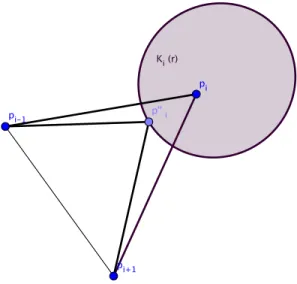
Proof of Claim 3. For each vertex qiconsider the triangle ∆i whose vertices are qi−1, qi, qi+1. By the transversality condition ∆iis a nondegenerate triangle and so lies in a unique affine planes Pi⊂ E. The solid cylinder Li(r) intersects Pi in a convex domain Ki(r) (the interior of an ellipse) containing the vertex qi, and for r sufficiently small the other two vertices of our triangle are not in Ki(r). See
Figure 2. The curve shortening process of Claim 3
figure 2. Ki(r) ∩ ∆i ⊂ Pi is a convex planar domain whose boundary consists of three arcs, two being line segments forming part of the edges of ∆i and the third curved arc Ci (a subarc of the ellipse) lying in the interior of ∆i. Choose any point qi′′ ∈ Ci on this third arc. Then q′′i ∈ Zi(r). But q′′i is in the interior of our triangle, and so by a general property of interior points of triangles we have that ∣qi−1− q′′
i∣ + ∣q′′i − qi+1∣ < ∣qi−1− qi∣ + ∣qi− qi+1∣. See figure2 again.
It follows that the replacement of vertex qi by qi′′ leaving all other vertices of q unchanged shortens the polygonal path. Indeed, only the edge lengths of the two edges incident to the changed vertex change and the sum of these two de-crease. Write this replacement process as q ↦ σi(q). Apply this polygonal curve shortening process consecutively, vertex-by-vertex, q↦ σ1(q) ↦ σ2(σ1(q)) ↦ . . . ↦ σk(. . . (σ1(q)) . . .)) = q′′. Each replacement shortens the path. The kth application yields a path q′′∈ P(r) all of whose corners q′′
i lie on their respective boundary sets Zi(r) and which is shorter than the original path q. ◻ (for the proof of Proposi-tion3).
6.1. Relation to proofs of theorems 1, 2. The r-thickened dynamics is de-terministic and symplectic. The graph of its time T flow is, morally speaking, a Lagrangian graph. This graph is partitioned up into pieces according to the itineraries of the trajectories. In some sense, which we are purposely vague on, our Lagrangian relations of theorems1 and 2, are the limits r → 0 and T →∞ of the
pieces of this graph. Among the problems faced in turning this idea into a complete proof is the fact that the flow is not continuous due to the instantaneous velocity changes suffered at collisions.
7. Conservation Laws, Symmetries, and Scaling.
Solutions to the N -body problem enjoy conservation of linear and angular mo-mentum. We expect that our N -body billiard trajectories to obey these same conservation laws. They do. We show derive the laws from the group invariance of the collision subspaces. We end this section with a remark on a scaling symme-try for billiard trajectories and what it implis for the closures of our Lagrangian relations in theorem1.
7.1. Momentum maps for free motion and its restrictions. The usual linear and angular momentum are the components of the momentum map for the group of rigid motions of the underlying Euclidean space. We take, to start with, the full group of rigid motions of our E, and later restrict to subgroups mapping the collision spaces to themselves.
The group Iso(E) of rigid motions of E splits into translations and rotations. Write Lie(Iso(E))∗for the dual of the Lie algebra of this Lie group. Using the inner product on E we have canonical identifications: T∗E= E × E and Lie(Iso(E))∗ = Lie(Iso(E)) = E ⊕ Λ2
E. The full momentum map is then the map Φ = (P, J) ∶ E× E → E ⊕ Λ2
E whose first (translational) factor P(x, v) = v we call the “full” linear momentum and whose second (rotational) factor Jrot(x, v) = x∧v we call the ‘full’ angular momentum and is that for the full rotation group.
Free (=straight line) motion(x, v) ↦ (x + tv, v) is a Hamiltonian flow on E × E which has the full momenta as conserved quantities.
Now restrict attention to the Lie subgroup of those g∈ Iso(E) such that g(L) = L for each L∈ L. Being a subgroup of Iso+(E), this subgroup also acts symplectically on the phase space E × E and has its own momentum map which is well-known to be the composition of the previous full momentum map Φ with the orthogonal projection onto our subgroup’s Lie algebra. In this way we get linear and angular momenta associated to our collision-preserving subgroup. :
Ptr(x, v) = πtr(v) ∈ Ltr and
J(x, v) = π(x ∧ v) ∈ Lie(H)
where πtr ∶ E → Ltr projects onto the translational part of our subgroup and π ∶ Λ2
E → Lie(H) projects onto its rotational part. In the next two subsections we compute these projections and derive their conservation consequences.
7.2. Linear Momentum and Translation invariance. The translational part of our collision-preserving subgroup is:
(20) Ltr= ⋂
L∈L L.
In other words, Ltr is precisely the subgroup of translations of E which maps each Lonto itself. Write πtr∶ E→ Ltr for the orthogonal projection onto this subspace, as above, we have:
Proposition 4. The ‘total linear momentum” πtr(v) is constant along each billiard trajectory.
Proof. At each collision we have πL(v−) = πL(v+). But Ltr⊂ L for all L ∈ L. So πtr(v−) = πtr(v+) at each collision: the total momentum remains unchanged at each collision and thus πtr(v) is constant along any given billiard trajectory. ◻ N -body billiard momentum conservation In N -body billiards the inter-section of all of the ∆ij consists of the d-dimensional subspace consisting of all vectors of the form(z, z, . . . , z), z ∈ Rd. It is the subspace of E= (Rd)N generated by the translation group of Rd. The projection of a velocity v ∈ (Rd)N onto this subspace, relative to the mass metric, is (v1, . . . , vN) ↦ Σmava which co-incides with total linear momentum.
7.3. Angular Momentum and Rotational Invariance. Now we consider the rotational part of our collision-preserving subgroup. Denote this subgroup as H⊂ O(E) so that H consists of all rotations which map the collision subspaces to themselves. We write πH∶ Λ2
E→ Lie(H) for the orthogonal projection, identifying Lie(H) with a linear subspace of Λ2(E). Use the naturally induced invariant inner product on Λ2(E). On bivectors v ∧ w the squared length for this inner product is (21) ⟨v ∧ w, v ∧ w⟩ = det ( ⟨⟨v, w⟩ ⟨w, w⟩ )v, v⟩ ⟨w, v⟩
Proposition 5. The ‘total angular momentum” πH(x, v) is constant along each billiard trajectory.
Proof. Let ξ ∈ Lie(H). Thus etξ ∈ H is a one-parameter family of rotations leaving each L invariant. The ξ-component of the full angular momentum is
Jξ(x, v) = ⟨x ∧ v, ξ⟩ where ⟨⋅, ⋅⟩ is the inner product on so(E) ≅ Λ2
E just described. Since x∧ v is constant along straight line motions, Jξ(x, v) remains constant along the straight line segment parts of a billiard trajectory. We must show that it remains unchanged at collisions. The jump in Jξ at a collision with an L at q∈ L is:
Jξ(q, v+) − Jξ(q, v−) = ⟨q ∧ (v+− v−), ξ⟩
Now from πL(v+) = πL(v−) we have that v+− v−∈ L⊥. Thus q∧ (v+− v−) ∈ L ∧ L⊥⊂ Λ2
E. Our proposition now follows from the computational lemma: Lemma 5. If ξ∈ Lie(H), q ∈ L and v ∈ L⊥ then ⟨q ∧ v, ξ⟩ = 0.
Proof of lemma. Using bilinearity of the inner product and formula (21) one verifies that for any ξ∈ Λ2
E we have
⟨q ∧ v, ξ⟩ = ⟨ξ(v), q⟩
where on the right-hand side we view are viewing ξ as a skew symmetric map ξ ∶ E→ E using the canonical identification Λ2
(E) ≅ so(E). (Under this identification the bivector q∧v becomes the linear transformation e ↦ (q ∧v)(e) = ⟨v, e⟩q −⟨q, e⟩v of E.) It follows that we also have
⟨q ∧ v, ξ⟩ = −⟨ξ(q), v⟩
Now if ξ∈ Lie(H) then etξ∈ H is a one-parameter family of rotations leaving each L invariant. Differentiating, we see that if q∈ L then ξ(q) ∈ L. But in the lemma
v∈ L⊥ so that−⟨ξ(q), v⟩ = 0. ◻
N body billiards. The group H = O(d) acts diagonally on the N-body con-figuration space (Rd)N leaving each ∆ij invariant. The mass-metric projection of
q∧ v ∈ so((Rd)N) = so(E) to Lie(H) = Λ2Rd is πH(q ∧ v) = ΣN
a=1maqa∧ va ∈ Λ2Rd, the usual formula for the total angular momentum. We have that total angular momentum is conserved for N -body billiards.
7.4. Scaling and the Scattering map as a Legendrian Map. If q(t) is a billiard trajectory with itinerary L1L2. . . Lkthen so is λq(λt) ∶= qλ(t), λ > 0. Letting λ→ 0 brings all the collision points qiof qλto the origin. In this way we see that the closure of the Lagrangian relation R for B(L1L2. . . Lk) (see theorem1) contains points lying in the Lagrangian relation for total collision described in example1 -namely the product of the two zero sections of T∗S(E) = LINES(E).
Scaling acts on pairs (q, v) ∈ E × Ev by λ(q, v) = (λq, v). Directions are left un-changed while ‘impact parameters’ q are scaled. Let ˜R = ˜R(L1. . . Lk) be the “unre-duced” Lagrangian relation of theorem2. The scale invariance ofB(L1L2. . . Lk) im-plies that ˜R is scale-invariant: (qA, vA), (qB, vB) ∈ ˜R ⇐⇒ ((λqA, vA), (λqB, vB)) ∈
˜
R. In other words, the Lagrangian relation is a scale-invariant submanifold of (E × Ev) × (E × Ev).
Scaling commutes with reduction, and so induces a scaling action on T∗S(Ev)× T∗S(Ev) which leaves the Lagrangian relation R of theorem1invariant. In terms of the coordinates on LIN ES(E) ≅ T∗S(Ev) discussed in subsection1.2.6, scaling acts again by (v, Q) ↦ (v, λQ). Thus we expect to be able to form the quotient by this action to arrive at a submanifoldR/R+⊂ (T∗S(E
v) × T∗S(Ev))/R+. The latter is a nice manifold provided we delete its zero section before forming the scaling quotient. Indeed, for any manifold X, let ZX⊂ T∗X denote the zero section of its cotangent bundle. Then(T∗X∖Z
X)/R+= P(T∗X) is a canonical contact manifold which fibers over X with fibers RPn−1’s, n= dim(X). (See [Arnold, Appendix 4].) We apply this observation to X = S(Ev) × (S(Ev), using T∗(S(Ev) × T∗S(Ev) = T∗(S(Ev) × (S(Ev)) to arrive at:
Theorem 5. If the itinerary has length greater than 1 then the quotient R/R+ of the Lagrangian relation R of theorem 1 by the scaling group R+ is a submanifold of PT∗(S(E
v) × (S(Ev)) of dimension 2dim(E) − 3 which is Legendrian relative to the (nonstandard) contact form
Θ= ⃗Q−⋅ d⃗v−− ⃗Q+ ⋅ d⃗v+.2
The projections to the incoming and outgoing velocity spheres are scale invariant maps and combine to yield the Legendrian fibration
π−× π+∶ PT∗(S(Ev) × (S(Ev)) → S(Ev) × S(Ev)
under which the image ofR/R+ is a (possibly singular) hypersurface provided it is transverse to the fiber at some point
Proof. We first check thatR does not intersect the zero section. If Q = 0 then 0= q1+ tv− which is only possible if either q1= 0 or v−∈ L1 with v−= −q1/t. The latter is impossible since this would imply that the whole incoming line ℓ−⊂ L1. If the itinerary has length 2, the former is also possible, since if q1= 0, then q1∈ L2 as well, which is excluded by our definition of belonging toB. Thus the quotient R/R+is a well-defined submanifold of PT∗(S(Ev) × (S(Ev)).
2
The form itself varies under scaling so is not well-defined as a one-form on PT∗(S(E
v) ×
(S(Ev)). The form is to be viewed projectively: its zero locus, which is the contact distribution,
Next we check the Legendrian condition and at the same time work out the contact form. Write D = ⃗Q−∂ ⃗Q∂
− + ⃗
Q−∂ ⃗Q∂
− for the Euler vector field, this being
the vector field whose flow is dilation (with λ= et if t is the flow parameter). Let Ω = ω−− ω+ be the symplectic form with respect to which R is Lagrangian. A standard construction from contact and symplectic geometry suggests forming the one-form Θ= iDΩ which a direct computation shows that Θ is the one-form stated in the theorem. Since R is scale invariant, D is tangent to R and consequently Θ(v) = Ω(D, v) = 0 for any other vector v tangent to R. This proves that R/R+ is Legendrian relative to Θ.
Finally, ifR/R+is transverse to the fibers of the fibration, then π−× π
+maps it locally diffeomorphically onto a hypersurface. The projection andR/R+ are both algebraic so if the Legendrian submanifold is transverse at one point it is transverse at almost every point and the image of each component is a singular hypersurface. ◻
Remark. IfR/R+is nowhere transverse to the fiber then it is mapped to a subvariety of codimension greater than 1 within the product of the spheres.
Remark. We can summarize the discussion of this subsection as saying that the map q ↦ (v−, v+) which sends a billiard trajectory to its incoming and outgoing velocities is a “Legendrian map”. Arnol’d [Arnold, Appendix 16, p. 487] calls the restriction of a Legendrian fibration to a Legendrian submanifold a “Legendrian map” and its image a “front” as in “wave-front. So the “scattering map” π−× π+ restricted to R/R+ is a Legendrian map and its image, the ‘scattering front’ will be an interesting singular hypersurface within the product of the incoming and outgoing velocity spheres. See subsection8.2below.
8. Examples
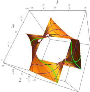
8.1. Origami unfoldings. Suppose thatL consists of lines, so that d = dim(E)−1. Let q∈ B(L1L2. . . Lk) be a trajectory. Then each qi∈ Li is nonzero, for otherwise qi∈ Li+1which is forbidden. Assume k> 1. Edge qiqi+1 of our k+ 1-gon q joins the rays Ð0qi→andÐÐ→0qi+1 and hence lies in the plane Pi spanned by 0, qi, qi+1. Within this plane the edge lies within the sector Si bounded by these two rays. (By a “sector” we mean a planar convex region bounded by two rays.) Let θi = angle(qi0qi+1) denote the opening angle of this sector. Thus the interior part q1q2...qk of our billiard trajectory lies on a polygonal cone within E whose faces are the sectors S1. . . Sk−1 glued together along the rays 0qi⊂ Li. We can “unfold” this cone onto a fixed plane, thus forming a big sector which is made of congruent copies of our sectors S1, S2, . . . , Sk−1joined along their shared rays; see figure3.
The opening angle of this big developed sector is β= θ1+ θ2+ . . . θk−1.
Our billiard trajectory unfolds onto this developing plane as well. The billiard condition (1) is precisely that this unfolded trajectory is a straight line segment on this developing plane. To reiterate,
The billiard segment q1. . . qk becomes a straight line segment drawn on our big sector which is the flattened polyhedral cone!
Figure 3. Left: Origami in E. Right: Origami unfolded
Proof. For if a straight line enters in to one part of a sector through one ray boundary and leaves through the other ray boundary then the opening angle of the sector cannot be greater than π. Said differently, the developed sector will not be
convex if β> π. ◻
Set βi= angle(Li, Li+1) so that βi is the minimum of θi and π− θi. Thus β≥ Σβi. Corollary 2. Set θmin= min(angle(L, M)), the minimum taken over all L, M ∈ L, L≠ M. There are no itineraries of length greater than 1 + ⌊π/θmin⌋.
Proof. Indeed since βi≥ θminwe have that β≥ (k − 1)θminso that π≥ (k − 1)θmin and thus the number of intersection k satisfies(π/θmin) ≥ k − 1 . ◻ Projecting the incoming and outgoing velocities onto our developing plane we get information on their angles from the unfolded figure.
Corollary 3. Consider the angle θ0 between the incoming ray (direction vA) and the line L1, the angle oriented so as to be the angle between q1 and−vA. Similarly consider the angle θk between the final collision line Lk and the outgoing ray (di-rection vB), that angle oriented so as to be between the vector qk and vector vB. Then:
θ0+ β + θk= π; i.e. Σki=0θi= π.
Proof. Indeed, add on open planar sectors with the plane AL1 and LkB to the polygonal figure described above, and flatten it. Our billiard trajectory is a straight line on the resulting plane and the angle sum, simply the opening angle of a line,
is π. ◻
We can now give a precise description of the Lagrangian relation ˜R(L1. . . Lk). For the relation to be nonempty we require Σβi< π. For each i we consider two possible angles, βi and π− βi. In all then, we have a collection of 2k−1 angles θi, each θi being either βi or π− βi. Among all these angle selections θ1, θ2, . . . , θk−1 we only consider those for which β∶= Σθi< π. Now fix such a selection. If our incoming line hits L1at an angle θ0, as defined in the corollary, then our outgoing line must leave at angle θk = π − β − θ1. Let q1, qk be the points where the incoming line hits L1