The Informational Content of Over-the-Counter Currency Options

Texte intégral

(1)2004s-16. The Informational Content of Over-the-Counter Currency Options Peter Christoffersen, Stefano Mazzotta. Série Scientifique Scientific Series. Montréal Avril 2004. © 2004 Peter Christoffersen, Stefano Mazzotta. Tous droits réservés. All rights reserved. Reproduction partielle permise avec citation du document source, incluant la notice ©. Short sections may be quoted without explicit permission, if full credit, including © notice, is given to the source..

(2) CIRANO Le CIRANO est un organisme sans but lucratif constitué en vertu de la Loi des compagnies du Québec. Le financement de son infrastructure et de ses activités de recherche provient des cotisations de ses organisations-membres, d’une subvention d’infrastructure du ministère de la Recherche, de la Science et de la Technologie, de même que des subventions et mandats obtenus par ses équipes de recherche. CIRANO is a private non-profit organization incorporated under the Québec Companies Act. Its infrastructure and research activities are funded through fees paid by member organizations, an infrastructure grant from the Ministère de la Recherche, de la Science et de la Technologie, and grants and research mandates obtained by its research teams. Les organisations-partenaires / The Partner Organizations PARTENAIRE MAJEUR . Ministère du développement économique et régional [MDER] PARTENAIRES . Alcan inc. . Axa Canada . Banque du Canada . Banque Laurentienne du Canada . Banque Nationale du Canada . Banque Royale du Canada . Bell Canada . BMO Groupe Financier . Bombardier . Bourse de Montréal . Caisse de dépôt et placement du Québec . Développement des ressources humaines Canada [DRHC] . Fédération des caisses Desjardins du Québec . GazMétro . Hydro-Québec . Industrie Canada . Ministère des Finances [MF] . Pratt & Whitney Canada Inc. . Raymond Chabot Grant Thornton . Ville de Montréal . École Polytechnique de Montréal . HEC Montréal . Université Concordia . Université de Montréal . Université du Québec à Montréal . Université Laval . Université McGill ASSOCIE A : . Institut de Finance Mathématique de Montréal (IFM2) . Laboratoires universitaires Bell Canada . Réseau de calcul et de modélisation mathématique [RCM2] . Réseau de centres d’excellence MITACS (Les mathématiques des technologies de l’information et des systèmes complexes) Les cahiers de la série scientifique (CS) visent à rendre accessibles des résultats de recherche effectuée au CIRANO afin de susciter échanges et commentaires. Ces cahiers sont écrits dans le style des publications scientifiques. Les idées et les opinions émises sont sous l’unique responsabilité des auteurs et ne représentent pas nécessairement les positions du CIRANO ou de ses partenaires. This paper presents research carried out at CIRANO and aims at encouraging discussion and comment. The observations and viewpoints expressed are the sole responsibility of the authors. They do not necessarily represent positions of CIRANO or its partners.. ISSN 1198-8177.

(3) The Informational Content of Over-the-Counter Currency Options* Peter Christoffersen†, Stefano Mazzotta Résumé / Abstract Les dirigeants et les participants du marché examinent souvent l'information prévisionnelle des options sur devises lorsqu’ils produisent des estimations quant aux développements futurs des taux de change étrangers. Les volatilités implicites des options peuvent être employées comme prévisions de la volatilité réalisée et les prévisions d'intervalles et de densités peuvent être extraites à partir de stellages (strangles) et de cylindres (risk-reversals). Le but de cet article est d'évaluer la qualité de telles prévisions des volatilités, intervalles et densités. Nous analysons des prévisions basées sur les options à partir d'une base de données unique comprenant 10 ans de données quotidiennes sur des prix d’options sur devises hors cote (OTC). Nous constatons que les volatilités implicites du marché hors cote expliquent une part beaucoup plus importante de la variation de la volatilité réalisée que celle qui a été mise en évidence précédemment dans les études basées sur des options transigées sur les marchés cotés. Nous constatons également que les prévisions d'intervalles de grande amplitude sont souvent mal spécifiées tandis que des prévisions d'intervalles de faible amplitude sont bien caractérisées. De plus, nous constatons que les prévisions de densité basées sur les options sont en général rejetées. L'étude graphique des prévisions de densité suggère que bien que les sources de rejets varient avec la devise, la spécification erronée des queues de distribution est une source d'erreur commune. Mots clés : devises, volatilité, intervalle, densité, prévisions. Policy makers and market participants often consider the forward-looking information in currency option valuations when making assessments about future developments in foreign exchange rates. Option implied volatilities can be used as forecasts of realized volatility and interval and density forecasts can be extracted from strangles and risk-reversals. The purpose of this paper is to assess the quality of such volatility, interval and density forecasts. We analyze option-based forecasts from a unique dataset consisting of over 10 years of daily data on over-the-counter (OTC) currency option prices. We find that the OTC implied volatilities explain a much larger share of the variation in realized volatility than has been found previously in studies relying on market-traded options. We also find that wide-range interval forecasts are often misspecified whereas narrow-range interval forecasts are well specified. Finally, we find that the option-based density forecasts are rejected in general. Graphical inspection of the density forecasts suggests that while the sources of rejections vary from currency to currency misspecification of the distribution tails is a common source of error. Keywords: Foreign exchange, volatility, interval, density, forecastings.. * We have benefited from several visits to the External Division of the European Central Bank whose hospitality is gratefully acknowledged. Very useful comments were provided by Torben Andersen, Lorenzo Cappiello, Olli Castren, Bruce Lehmann, Filippo di Mauro, Stelios Makrydakis, Nour Meddahi and Neil Shephard. The OTC volatilities used in this paper were provided by Citibank N.A. The usual disclaimer applies. † Corresponding author: Peter Christoffersen is at the Faculty of Management, McGill University, 1001 Sherbrooke Street West, Montreal, Quebec, Canada H3A 1G5, Phone: (514) 398-2969, Fax: (514) 398-3876, Email: peter. christoffersen@mcgill.ca, Web: www.christoffersen.ca..

(4) 1. Introduction Policy makers and market participants often consider the forward-looking information in currency option valuations when making assessments about future developments in foreign exchange rates.1 Option implied volatilities can be used as forecasts of realised volatility and interval and density forecasts can be extracted from strangles and risk-reversals. The purpose of this paper is to assess the quality of such volatility, interval and density forecasts. Our work is based on a very unique database consisting of more than ten years of daily quotes on European currency options from the OTC market. The OTC quotes include at-the-money implied volatilities, strangles and risk-reversals on the dollar, yen and pound per euro2 as well as on the yen per dollar. From this data we have constructed daily 1-month interval and density forecasts using the methodology in Malz (1997). The main findings of the paper are as follows: First and foremost, we find that the OTC implied volatilities explain a much larger share of the variation in realized volatility than has been found previously in studies relying on market-traded options. Second, we find that widerange interval forecasts are often misspecified whereas narrow-range interval forecasts are well specified. Third, we find that the option-based density forecasts are rejected in general. Graphical inspection of the density forecasts suggests that while the sources of rejections vary from currency to currency misspecification of the distribution tails is a common source of error. Our paper aims to fill two gaps in the literature. First, to our knowledge, the empirical performance of option-based interval and density forecasts has not been systematically explored so far. Second, while there is a considerable literature on implied volatility forecasts from market-traded options, OTC data have only recently been employed.3 Early market-data based contributions include Beckers (1981), Canina and Figlewski (1993), Lamoureux and Lastrapes (1993), and Jorion (1995), and more recent work include Christensen and Prabhala (1998), Fleming (1998), Blair, Poon, and Taylor (2001), and Neely (2003). One of our contributions consists of analyzing OTC options which turn out to have impressive volatility prediction properties. OTC options are quoted daily with a fixed maturity 1. See for example Bank for International Settlements (2003), Bank of England (2000), International Monetary Fund. (2002), and OECD (1999). 2. Prior to January 1, 1999 these were denoted in DEM.. 3. See Pong, Shackleton, Taylor and Xu (2004) and Covrig and Low (2003).. 2.

(5) (say one month) whereas market-traded options have rolling maturities which in turn complicate their use in fixed-horizon volatility forecasting. In addition to volatility forecasts we evaluate option-based interval and density forecasts which are widely used by practitioners but which have not been systematically assessed so far. OTC options are quoted daily with fixed moneyness in contrast with market-traded options which have fixed strike prices and thus timevarying moneyness as the spot price changes. This time-varying moneyness complicates the use of market-traded options for interval and density forecasting in that the effective support of the distribution is changing over time. Finally, the trading volume in OTC options is often much larger than in the corresponding market traded contracts which in turn renders the OTC quotes more reliable for information extraction. The remainder of the paper is structured as follows. Section 2 defines the competing volatility forecasts we consider and describes the standard regression-based framework for volatility forecast evaluation. Section 3 presents results on the option-implied and historical return-based volatility forecasts of realized volatility. Section 4 suggests a method for evaluating interval forecasts from option prices and present results from this method. Section 5 suggests methods for evaluating density forecasts from option prices and present results from these methods. Finally, Section 6 discusses potential points for future research. 2. Volatility Forecast Evaluation In order to evaluate the informational content of the volatilities implied from currency options, we define the realized future volatility for the next h days to be. σ tRV ,h =. 252 h 2 ∑ Rt +i h i =1. in annualized terms, where Rt+i = ln(St+i/St+i-1) is the FX spot return on day t+i. This realized volatility (and its logarithm) will be our forecasting object of interest in this section.4 We will consider four competing forecasts of realized volatility. First and most importantly the implied volatility from at-the-money OTC currency options with maturity h, where h is either 1 month or 3 months corresponding to roughly 21 and 63 trading days respectively. Denote this options-implied volatility by σ tIV,h . 4. Later on we will consider realized volatilities calculated from 30-minute rather than daily returns.. 3.

(6) The other three volatility forecasts are derived from historical FX returns only. The simplest possible forecast is the historical h-day volatility, defined as 252 h 2 Rt − h + i = σ tRV ∑ − h, h h i =1. σ tHV ,h =. The historical volatility is a simple equal weighted average of past squared returns. We can instead consider volatilities that apply an exponential weighting scheme putting progressively less weight on distant observations. The simplest such volatility is the Exponential Smoother or RiskMetrics volatility, where daily variance evolves as ∞. σ~t2+1 = (1 − λ )∑ λi −1 Rt2−i +1 = λσ~t2 + (1 − λ )Rt2 i =1. Following JP Morgan we simply fix λ=0.94 for all the daily FX returns. The fact that the coefficients on past variance and past squared returns sum to one makes this model akin to a random walk in variance. The annualized forecast for h-day volatility is therefore simply 252σ~t2+1 σ tRM ,h =. Finally we consider a simple, symmetric GARCH(1,1) model, where the daily variance evolves as. σˆ t2+1 = ω + βσˆ t2 + αRt2 In contrast with the RiskMetrics model, the GARCH model implies a non-constant term structure of volatility. The unconditional variance in the model can be computed as. σˆ 2 =. ω 1−α − β. The conditional variance for day t+h can be derived as. σˆ t2+h|t = σˆ 2 + (α + β )h−1 (σˆ t2+1 − σˆ 2 ) And the annualized GARCH volatility forecast for day t+1 through t+h is thus. σ tGH ,h =. (. 252 h 2 σˆ + (α + β )i−1 σˆ t2+1 − σˆ 2 ∑ h i=1. 4. ).

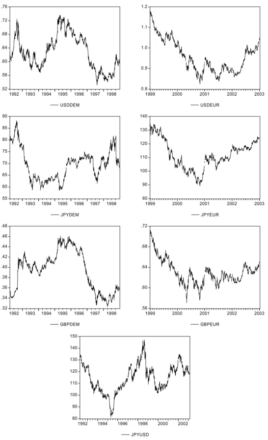
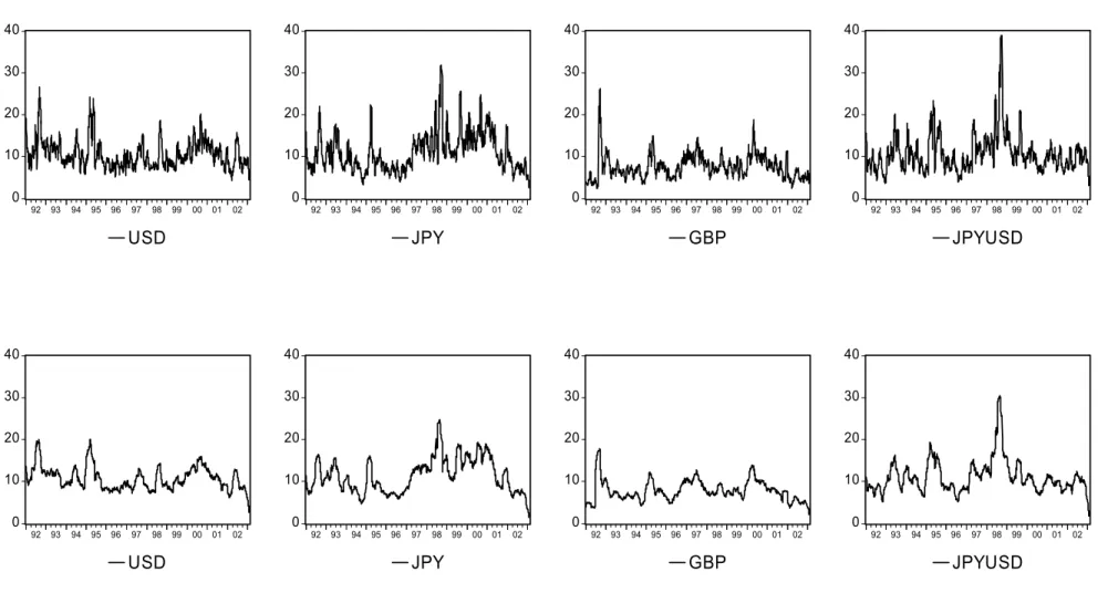
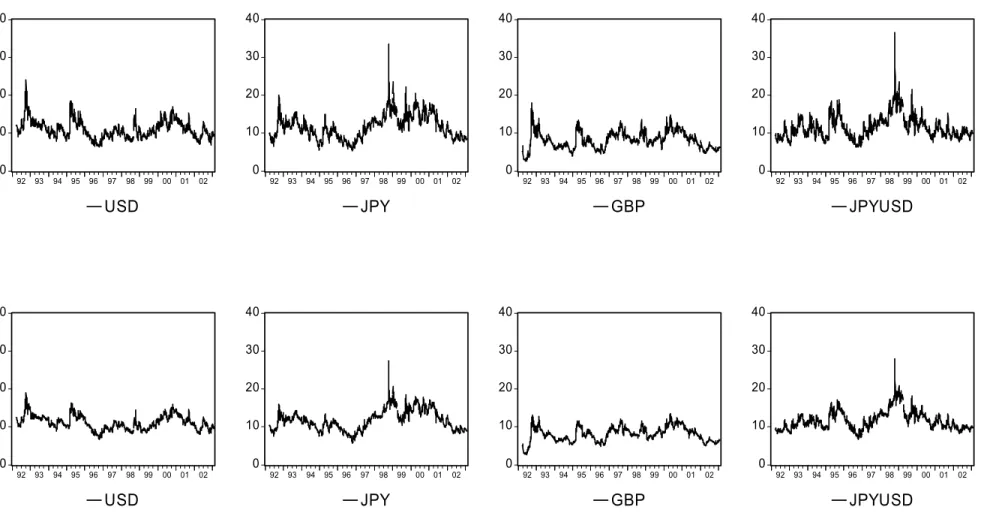
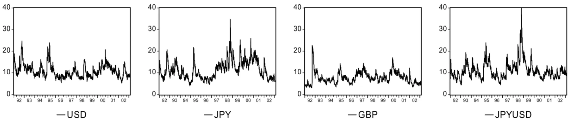
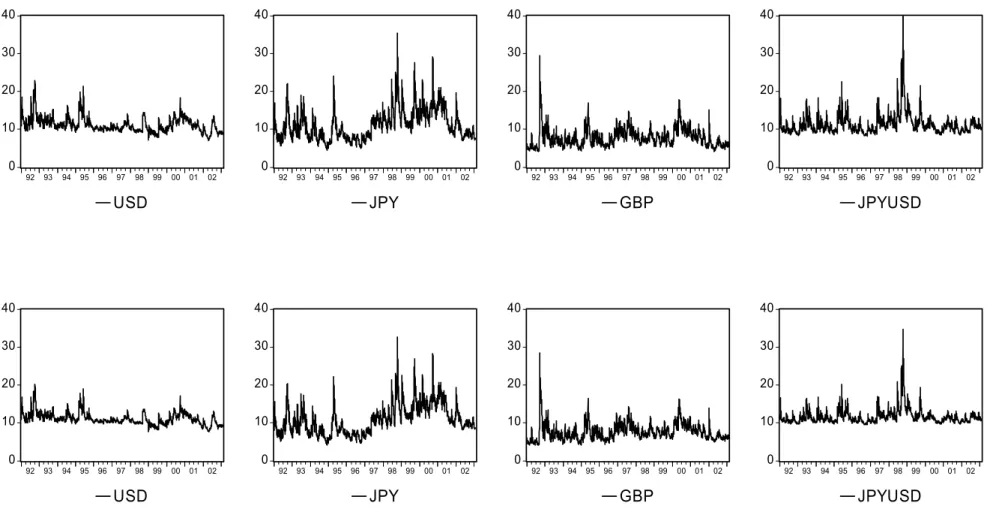
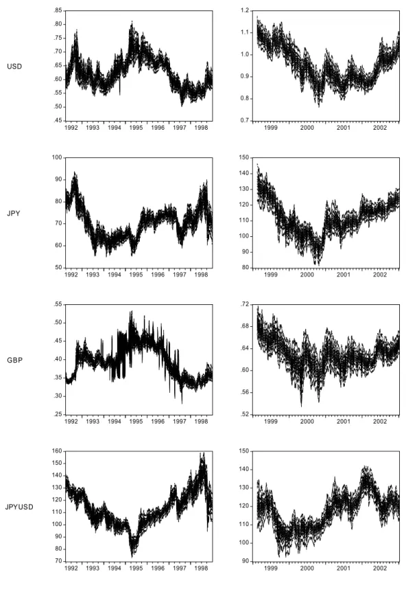
(7) The GARCH model will have a downward sloping volatility term structure when the current variance is above the long horizon variance and vice versa.5 Figure 1 shows the spot rates of the four FX rates analysed in this paper. Prior to the euro introduction in 1999 we observe FX options denoted against the Deutschmark (DEM) and we will therefore work with the DEM spot rates prior to the euro introduction as well. Prior to January 1, 1999 we use DEM options to forecast DEM volatility and afterwards we use euro options to forecast euro volatility. The five volatility specifications including the realized volatility are plotted in Figures 2-5. Each page corresponds to a particular volatility specification and each column on a page represents an FX rate. The top row shows the 1-month volatility and the bottom row the 3-month volatility. Notice that the RiskMetrics volatilities in Figure 4 are identical for 1-month and 3month maturities as the random-walk nature of this specification implies a flat volatility term structure. We are now ready to assess the quality of the different volatility forecasts. This will be done in simple linear predictability regressions. We first run four univariate regressions for each currency j j σ RV t , h = a + bσ t , h + ε t , h , for j = IV, HV, RM , GH. The purpose of these univariate regressions is to assess the fit through the adjusted R2 and to check how close the estimates of a are to 0 and how close the estimate of b are to 1. Bollerslev and Zhou (2003)6 point out that if the volatility risk is priced in the options markets then we should expect to find a positive intercept and a slope less than one in the above regression. Nevertheless, for someone using implied volatility in the real time monitoring of FX movements, the intercept and slope coefficients are informative of the size of the bias and efficiency respectively of the forecasts.. 5. The GARCH model contains parameters which must be estimated. We do this on rolling 10-year samples starting. in January 1982 and using QMLE. Each year we forecast volatility one-year out-of-sample before updating the estimation sample by another calendar year of daily returns. The euro volatility forecasts are constructed using synthetic euro rates in the period prior to the introduction of the euro. 6. See also Bandi and Perron (2003) and Chernov (2003).. 5.

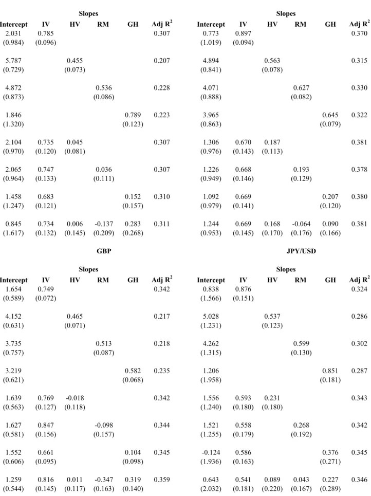
(8) In addition we will run three bivariate regressions including the implied volatility forecast as well as each of the three return-based volatility forecasts in turn. Thus we have IV j IV , j σ RV t , h = a + bσ t , h + cσ t , h + ε t , h , for j = HV, RM, GH. The purpose of the bivariate regressions is to assess if the return-based volatility forecasts add anything to the market-based forecasts implied from currency options. Finally, we run a regression including all the four volatility forecasts in the same equation. The purpose of this regression is to assess the relative merits of the different volatility forecasts. We will run all regressions for h=21 and 63 corresponding to the 1-month and 3-month option maturities. We will also run all regressions in levels of volatility as above as well as in logarithms. Due to the volatilities being strictly positive, the log specification may have error terms, which are better behaved than those from the level regressions. 3. Volatility Forecast Evaluation Results. Tables 1 and 2 report the regression point estimates as well as standard errors corrected for heteroskedasticity and autocorrelation using GMM. Throughout this paper we apply the robust Newey-West weighting matrix with a prespecified bandwidth equal to 21 days for the 1-month horizon (Table 1) and 63 days for the 3-month horizon (Table 2). We also report the regression fit using the adjusted R2. Several strong and interesting empirical regularities emerge. First, the regression fit is very good in all cases. Jorion (1995) reports R2 in the region 0.10-0.15 for the USD/JPY, USD/DEM and USD/CHF using implied volatility forecasts. We get instead R2 of 0.30-0.38 for the 1-month maturity and 0.16-0.35 for the 3-month maturity case. Second, comparing the R2 across the univariate forecast regressions we see that the implied volatility is the best volatility forecast. This result holds across currencies and horizons. Third, comparing the slope estimates across the bivariate forecast regressions where the implied volatility forecast is included along with each of the other three forecasts, the implied volatility always has the highest slope. Thus, in the cases when GARCH has a higher slope in the univariate regression the bivariate regressions including the IV and GARCH forecasts always assign a larger slope to the IV forecast. The fact that GARCH-based forecasts sometimes have a slope closer to one than do the implied volatility forecasts is not surprising given the price of volatility risk argument in Bollerslev and Zhou (2003) and others. But it is interesting to note 6.

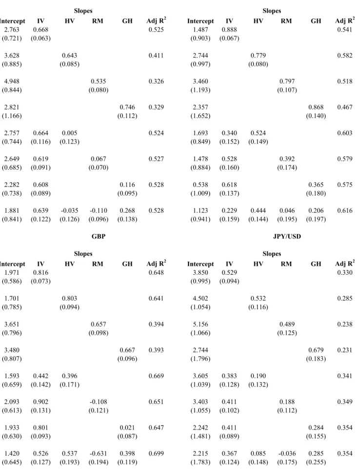
(9) that the R2 is higher for the implied volatility forecasts even in the cases where its slope is lower than that of the GARCH-based forecasts. Fourth, comparing the slope estimates across the multivariate forecast regressions where all four forecasts are included simultaneously the implied volatility has the highest slope. This result holds across currencies and horizons. Fifth, comparing across the horizon forecasts it appears perhaps not surprisingly that the 1-month forecasts have higher R2 than the 3-month forecasts. Finally, the slope coefficient is often insignificantly different from one for the IV forecasts, and its intercept is often insignificantly different from zero. Tables 3 and 4 contain the same set of regressions as Tables 1 and 2, but now run on the euro sample (i.e. post January 1, 1999) only, and furthermore relying on 30-minute intraday returns rather than daily returns to compute the one and three month realized volatilities. The objective of Tables 3 and 4 is to see if the post-euro sample is different from the full sample period which straddles the introduction, and furthermore to assess the value of using highfrequency returns in volatility forecast evaluation. The theoretical benefits of doing so have been documented in Andersen and Bollerslev (1998) and Andersen, Bollerslev and Meddahi (2003) who show that the R2 in the regressions we run will be significantly higher when proxying for true volatility using an intraday rather than daily return-based volatility measure. As pointed out by Alizadeh, Brandt and Diebold (2002), and Brandt and Diebold (2003) this theoretical benefit may in practice be outweighed by market microstructure noise, but relying on 30-minutes returns in very liquid markets as we do here should mitigate these problems. The results in Table 3 and 4 are broadly similar to those from the full sample but using high-frequency returns does lead to some new interesting findings. First, for the three euro cross currencies the regression fit is typically much better now. Due to the obvious structural break in 1999 this is perhaps not surprising. But it is still interesting that we now get R2 as high as 65% in the univariate regressions. Note that the R2 for the 3-month JPY/USD case is now slightly lower than before. It is therefore not simply the case the FX volatility has become more predictable as of late. Second, comparing the R2 across the univariate forecast regressions the implied volatility is typically the best volatility forecast. The exception is the EUR/JPY rate. Third, comparing the slope estimates across the bivariate and multivariate forecast regressions the implied volatility typically has the highest slope. It is interesting that the simple historical realized volatility. 7.

(10) forecast now sometimes has the highest slope.7 The added accuracy in this forecast from the intra-day returns is thus evident. In summary we find strong evidence that the implied volatility from FX options is useful in predicting future realized volatility at the one and three month horizons. The predictability is particularly strong for the euro cross rates in the recent period. In spite of the potential bias from volatility risk being priced in the options, the regression slope on the volatility forecasts are often quite close to one. Perhaps the most striking finding in Tables 1-4 is the high level of R2 found in the implied volatility regressions. It appears that the volatility implied in the OTC options offer much more precise forecasts than the volatility implied from market-traded options, which have been analyzed in previous studies. We suspect that the so-called telescoping bias arising from the rolling-maturity structure of market-traded options (see Christensen, Hansen, and Prabhala, 2001) could be part of the reason. Furthermore, the fact that OTC options are quoted daily with a fixed moneyness, as opposed to a fixed strike price, which ensures that the options used for volatility forecasting are exactly at-the-money each day. Finally, the large volume of transaction in OTC currency options compared with market traded options may offer additional explanation. 4. Interval Forecast Evaluation. The information in currency options may be useful not only for volatility forecasting but for spot rate distribution forecasting more generally. In this section we study the performance of one-month interval forecasts calculated from option prices and forward rates. The intervals are constructed from the option-implied densities which in turn are calculated using the estimation method in Malz (1997). The Malz methodology is based on a second order Taylor approximation to the volatility smile. The procedure forces the approximation of the implied volatility function to be exactly equal to the observed implied volatility for the three values of the Black-Scholes delta, namely .25, .50, and .75. We have computed conditional interval forecasts for the {0.45, 0.55} probability interval, as well as the {0.35, 0.65}, {0.25, 0.75}, {0.15, 0.85}, and the {0.05, 0.95} intervals. These. 7. The historical volatility forecast could potentially be improved further by estimating a slope coefficient thus. allowing for mean reversion in the forecast.. 8.

(11) forecasts are shown in Figure 6. Notice that the intervals for the GBP/DEM look excessively jagged in a large part of the pre euro sample. We now set out to evaluate the usefulness of the interval forecasts. To this end consider the following simple framework. Let the generic interval forecast be defined as. {L. t,h. ( pL ),U t , h ( pU )}. where pL and pU are the percentages associated with the lower and upper conditional quantiles making up the interval forecast. Consider now the indicator variable defined as 0, if St + h ∈ {Lt,h(pL ),U t,h(pU )} I t,h =  1, if not. Then if the interval forecast is correctly calibrated, we must have that E [I t ,h | X t ] = 1 − ( pU − p L ) ≡ p where Xt denotes a vector of information variables (and functions thereof) available on day t. If the interval forecast is correctly calibrated then the expected outcome of the future FX rate falling outside the predicted interval must be a constant equal to the pre-specified interval probability p. This hypothesis will be tested in a linear regression setup, but binary regression methods could have been used as well. Under the alternative hypothesis we have I t , h − p = a + bX t + ε t , h and the null hypothesis corresponds to the restrictions a=b=0. Running these regressions on daily data we again have to worry about overlapping observations, which we allow for using GMM estimation. Table 5 shows the results for the regression-based tests of the interval forecasts. The interval forecasts for the {0.45, 0.55}, {0.35, 0.65}, {0.25, 0.75}, {0.15, 0.85}, and the {0.05, 0.95} intervals are denoted by the probability of an observation outside the interval, i.e. p=.90, .70, .50, .30 and .10 respectively. We refer to these outside observations as hits. The zero/one hit sequence (less its expected value p) is regressed on a constant, the 21-day lagged hit and the 21day lagged 1-month implied volatility. The lagged hit is included to capture any dependence in the outside observations. The implied volatility is included to assess if it is incorporated 9.

(12) optimally in the construction of the interval forecast. If the interval forecast is correctly specified then the intercept and slopes should all be equal to zero. Table 5 reports coefficient estimates along with t-statistics again calculated using GMM. Below the solid line in each subsection of the table the average hit rate, which should be equal to p, is reported along with the t-statistic from the test that the average hit rate indeed equals p. All t-statistics larger than two in absolute value are denoted in boldface type. We also include Wald tests of the joint hypothesis that all the estimated coefficients are zero. The results in Table 5 can be summarized as follows. First, for the pound the average hit rate is significantly different from the pre-specified p for all but the narrowest interval (with outside probability equal to .90). The jagged pound intervals evident from Figure 6 are probably the culprit here. Second, for the other three FX rates, the average hit rate is typically not significantly different from the pre-specified p. The only notably exception is the wide-range intervals (with outside probability .10) where all but the JPY/EUR intervals are rejected. It thus appears that the interval forecast have the hardest time forecasting the tails of the spot rate distribution. Third, notice that no regression slopes are significant in the JPY/EUR case. No dependence in the hit sequence is apparent and the information in implied volatilities seems to be used optimally in this case. Fourth, while the interval forecasts for the JPY/EUR are well specified, the intervals for the other three forecasts are typically rejected. The slope on the 21-days lagged implied volatility is most often found to be significantly negative. This indicates that the hits tend to occur when the implied volatility was relatively low on the day the forecast was made. If the intervals had been using the implied volatility information optimally then no dependence should be found between the current implied volatility and the subsequent realization of the hit sequence. Table 6 reports the interval forecast evaluation results using data from the euro sample only. The results are now somewhat different and can be summarized as follows. First, the average hit rate is typically not significantly different from the pre-specified p with a couple of noteworthy exceptions: The average hit rate is rejected across all the four FX rates for the widest intervals. Again, it appears that the option implied densities have trouble capturing the tails of the distribution. For all four FX rates it is the case that the outside hit frequency is lower than it should be, thus the wide-range option-implied intervals are too wide on average.. 10.

(13) Second, the average hit rate is rejected in the two widest intervals for the pound, but in general the pound intervals are better calibrated in the euro sample than before. Third, the JPY/USD interval is now the most poorly calibrated interval. In summary we find that the option-implied interval forecast for the euro cross rates perform well in the post January 1, 1999 sample. The exception is the forecasts for the widest intervals, which tend to be too wide on average. The option-implied densities apparently have trouble capturing the tail behaviour of the spot rate distributions. The rejection of widest intervals and thus misspecification of the tails of the density forecasts should perhaps not come as a surprise. The density tails are estimated on the basis of an extrapolation of the volatility smile from the values for which option price information is available (that is for deltas equal to .25, .50, and .75). It appears that this extrapolation could be improved. We will pursue the topic of density forecasting in more detail in the next section. 5. Density Forecast Evaluation. The option-implied interval forecasts analysed above are constructed from the implied density, which contains much more information than the intervals alone. We would therefore like to evaluate the appropriateness of these density forecasts in their own right. Doing so is likely to yield some insights into the poor performance of the widest interval forecasts, which was noted above. We start off by outlining the general idea behind density forecast evaluation. Let Ft , h (S ) and f t ,h (S ) denote the cumulative and probability density function forecasts made on day t for the FX spot rate on day t+h. We can then define the so-called probability transform variable as U t ,h ≡ ∫. St + h. −∞. f t ,h (u )du ≡Ft ,h (S t + h ).. The transform variable captures the probability of obtaining a spot rate lower than the realization where the probability is calculated using the density forecast. The probability will of course take on values in the interval [0,1]. If the density forecast is correctly calibrated then we should not be able to predict the value of the probability transform variable Ut,h using information available at time t. That is we should not be able to forecast the probability of getting a value smaller than the realization. Moreover, if the density forecast is a good forecast of the true probability distribution then the estimated probability will be uniformly distributed on the [0,1] interval.. 11.

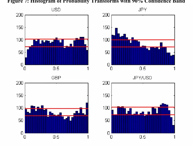
(14) 5.a Graphical Density Forecast Evaluation Figure 7 assesses the unconditional distribution of the probability transform variable Ut,h for each spot rate through a simple histogram. If the density forecast is correctly calibrated then each of the histograms should be roughly flat and a random 10% of the 31 bars should fall outside the two horizontal lines delimiting the 90% confidence band. It appears that the histograms display certain systematic differences from the uniform distribution. Notice in particular that the JPY/EUR histogram (top right panel) shows a systematically declining shape moving from left to right. This is indicative of the forecasted mean spot rate being wrong. There are too many observations where the realized spot rate lies in the left side of the forecasted distribution (and generates a Ut,h less than 0.5) and vice versa. In the USD/EUR case (top left panel) it appears that there are not enough observations in the two extremes, which suggests that the forecasted density has tails, which are too fat. This finding matches Table 5 where we found that the widest intervals were too wide for the USD/EUR. Finally, the JPY/USD distribution (bottom right panel) appears to be misspecified in the right tail. For certain purposes, including statistical testing, it is more convenient to work with normally distributed rather than uniform variables for which the bounded support may cause technical difficulties. As suggested by Berkowitz (2001)8 we can use the standard normal inverse cumulative density function to transform the uniform probability transform to a normal transform variable Z t , h = Φ −1 (U t , h ) = Φ −1 (Ft , h (St + h )). If the implied density forecast is to be useful for forecasting the physical density, it must be the case that the distribution of Ut,h is uniformly distributed and independent of any variable Xt observed at time t. Consequently the normal transform variable must be normally distributed and also independent of all variables observed at time t.. 8. See also Diebold, Gunther and Tay (1998) and Diebold, Hahn and Tay (1999).. 12.

(15) Figure 8 assesses the unconditional normality of the normal transforms by plotting the histograms with a normal distribution superimposed.9 The normal histograms typically confirm the findings in Figure 7 but also add new insights. While it appeared in Figure 7 that the GBP/EUR had fairly random deviations from the uniform distribution, it now appears that the normal transform is systematically skewed compared with the superimposed normal distribution. While the graphical evidence in Figures 7 and 8 is quite informative of the potential deficiencies in the option implied density forecasts, it may be interesting to formally test the hypothesis of the normal transforms following the standard normal distribution. We do this below. 5.b Tests of the Unconditional Normal Distribution We first want to test the simple hypothesis that the normal transform variables are unconditionally normally distributed. Basically, we want to test if the histograms in Figure 8 are significantly different from the superimposed normal distribution. The unconditional normal hypothesis can be tested using the first four moment conditions. [ ]. [ ]. [ ]. E [Z t ,h ] = 0, E Z t2,h = 1, E Z t3,h = 0, E Z t4,h = 3. We still need to allow for autocorrelation arising from the overlap in the data and so we estimate the following simply system of regressions Z t ,h = a1 + ε t(,1h) Z t2,h − 1 = a 2 + ε t(,2h) Z t3,h = a3 + ε t(,3h) Z t4,h − 3 = a 4 + ε t(,4h) using GMM and test that each coefficient is zero individually as well as the joint test that they are all zero jointly.10 In each case we allow for 21 day overlap in the daily observations. The results of these tests are reported in Tables 7 and 8. Table 7 tests for unconditional normality on the entire sample and Table 8 restricts attention to the post 1999 period.. 9. The superimposed normal distribution functions have different heights due to the different number of observations. available for each currency. 10. See Bontemps and Meddahi (2002) for related testing procedures.. 13.

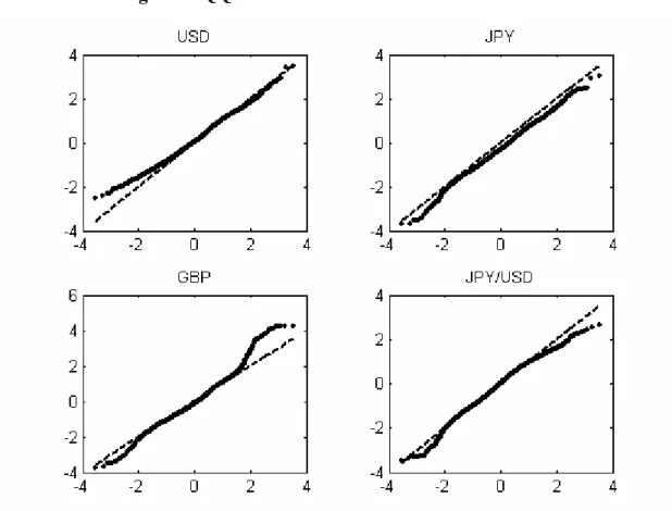
(16) Table 7 shows that while only a few of the individual moments are found to be significantly different from the normal counterpart, the joint (Wald) test that all moments match the normal distribution is rejected strongly in three cases and weakly in the case of the JPY/USD. The post 1999 results are very similar. Now the Wald test strongly rejects all four density forecasts. We thus find fairly strong evidence overall to reject the option-implied density forecasts using simple unconditional tests. In order to focus attention on the performance of the density forecasts in the tails of the distribution, we report QQ-plots of the normal transform variables in Figure 9. QQ-plots display the empirical quantile of the observed normal transform variable against the theoretical quantile from the normal distribution. If the distribution of the normal transform is truly normal then the QQ-plot should be close to the 45-degree line. Figure 9 shows that the left tail is fit poorly in the case of the dollar, and that the right tail is fit poorly in the case of the pound and the JPY/USD. In the case of the dollar there are too few small observations in the data, which is evidence that the option implied density has a left tail that is too thick. The pound has too many large observations indicating that the right tail of the density forecast is too thin. In the JPY/USD case the right tail appears to be too thick. These findings are also evident from Figure 7. Rejecting the unconditional normality of the normal transform variables is of course important, but it does not offer much constructive input into how the option-implied density forecasts can be improved upon. The conditional normal distribution testing we turn to now is more useful in this regard. 5.c Tests of the Conditional Normal Distribution We would like to know why the densities are rejected, and specifically if the construction of the densities from the options data can be improved somehow. To this end we want to conduct tests of the conditional distribution of the normal transform variable. Is it possible to predict the realization of the time t+h normal transform variable using information available at time t? If so then this information is not used optimally in the construction of the density forecast. The conditional hypothesis can be tested using the generic moment conditions. [. ]. [. ]. [. ]. E [Z t ,h f1 ( X t )] = 0, E Z t2,h f 2 ( X t ) = 1, E Z t3,h f 3 ( X t ) = 0, E Z t4,h f 4 ( X t ) = 3. 14.

(17) Choosing particular moment functions and variables these conditions can be implemented in a regression setup as follows Z t , h = a1 + b11Z t − h , h + b12σtIV + εt(1, h). ( ) +ε + b (σ ) + ε Z + b (σ ) + ε. Z t2,h − 1 = a2 + b21Z t2− h , h + b22 σtIV Z t3, h = a3 + b31Z t3− h , h Z t4,h − 3 = a4 + b41. 4 t − h, h. 32. 2. IV 3 t. 42. ( 2) t ,h. ( 3) t ,h. IV 4 t. ( 4) t ,h. where we include the lagged power of the normal transform as well as the power of the current implied volatility as regressors. We can now test that the regression coefficients are zero. Table 9 shows the estimation results of the regression systems for the four exchange rates. In line with previous results we find that the information in the implied volatility is not used optimally in the construction of the option-implied density forecast for the GBP/EUR. Table 10 shows the regressions from Table 9 run only on the euro sample. Comparing the two tables, it is evident that the clear rejection of the pound density forecasts in Table 9 is largely due to problems in the pre-euro sample. Restricting attention to the euro sample there is more evidence on the implied volatility being misspecified in the JPY/USD rate. Looking across Tables 9 and 10 we see that the Wald test of all coefficients being zero is strongly rejected for all four FX rates in both samples. It would therefore seem possible in general to improve upon the option-implied density forecasts studied here. 6. Conclusion and Directions for Future Work. We have presented evidence on the usefulness of the information in over-the-counter currency option for forecasting various aspects of the distribution of exchange rate movements. We focused on three aspects of spot rate forecasting, namely, volatility forecasting, interval forecasting, and distribution forecasting. While other papers have pursued volatility forecasting in manners similar to ours we believe to be the first to systematically investigate the properties of option-based interval and density forecasts. Furthermore, we believe to be the first to investigate long time series of volatilities from over-the-counter options, which we find to be much more useful for volatility forecasting than the market-traded options used in previous studies. The reasons for this important finding are likely to be 1) the so-called telescoping bias arising from rolling maturities in market-traded options is not an issue in the OTC options, 2) the time-. 15.

(18) varying moneyness in market-traded options, and 3) the volume of trades done over-the-counter is much larger than the exchange trading volume for currency options. Our other findings can be summarized as follows. First, the implied volatilities from currency options typically offer predictions that explain much more of the variation in realized volatility than do volatility forecasts based on historical returns only. Second, when combining implied volatility forecasts with return-based forecasts, the latter typically receive very little weight. Third, in terms of interval forecasting on the entire 1992-2003 sample, the optionimplied intervals are useful for the JPY/EUR but rejected for the other three currencies in the study. Fourth, focusing on the euro sample, the option-implied interval forecasts are generally useful. Two notable exceptions are the widest-range intervals with 90% coverage and the JPY/USD intervals in general. The 90% intervals tend to be too wide due to the misspecification of the tails of the forecast distribution. Fifth, when evaluating the entire implied density forecasts these are generally rejected. The graphical evidence again suggests that the tails in the distribution are typically misspecified. We thus conclude that the information implied in option pricing is useful for volatility forecasting and for interval forecasting as long as the interest is confined to intervals with coverage in the 10-70% range. The rejection of the widest intervals and the complete density forecast is of course interesting and warrants further scrutiny. The potential reasons are at least fourfold. First, the option contracts used may not have extreme enough strike prices to be useful for constructing accurate distribution tails. Second, the information in options could be used sub-optimally in the density estimates. Third, we could be rejecting the densities because certain information available at the time of the forecasts is not incorporated in the option prices used to construct the densities, i.e. option market inefficiencies. Fourth, the risk premium considerations, which were abstracted from in this paper could be important enough to reject the risk-neutral density forecasts considered. The misspecification of the mean in the case of the JPY/EUR rate suggests that an omitted risk premium could be the culprit in that case. For the other three currencies, however, Figure 9 suggests that the culprit is tail misspecification, which is likely to arise from the lack of information on deep in-the-money and deep out-of-the-money options. We round off the paper by listing some promising directions for future research. First, policy makers may be interested in assessing speculative pressures on a given exchange rate. The option implied densities can be used in this regard by constructing daily option-implied. 16.

(19) probabilities of say a 3% appreciation or depreciation during the next month. Second, the accuracy of the left and right tail interval forecast could be analyzed separately in order to gain further insight on the probability of a sizable appreciation or depreciation. Third, relying on the triangular arbitrage condition linking the JPY/EUR, the USD/EUR, and the JPY/USD, one can construct option implied covariances and correlations from the option implied volatilities. These implied covariances can then be used to forecast realized covariances as done for volatilities in Tables 1-4. Fourth, the misspecification found in the option-implied density forecasts may be rectified by assuming different tail-shapes in the density estimation or by incorporating returnbased information. Converting the risk-neutral densities to their statistical counterparts may be useful as well but will require further assumptions, which may or may not be empirically valid. Bliss and Panigirtzoglou (2004) present promising results in this direction.. 17.

(20) References. Alizadeh, S., M. Brandt, and F. Diebold, 2002, Range-Based Estimation of Stochastic Volatility Models, Journal of Finance 57, 1047-1091. Andersen, T., and T. Bollerslev, 1998, Answering the skeptics: Yes, standard volatility models do provide accurate forecasts, International Economic Review 39, 885-905. Andersen, T., T. Bollerslev, and N. Meddahi, 2003, Correcting the Errors: A Note on Volatility Forecast Evaluation Based on High-Frequency Data and Realized Volatilities, Working Paper, Duke University, Department of Economics. Andersen, T., T. Bollerslev, F. X. Diebold, and P. Labys, 2003, Modeling and Forecasting Realized Volatility, Econometrica 71, 579-626. Bandi, F., and B. Perron, 2003, Long memory and the relation between implied and realized volatility, Manuscript, University of Chicago. Bank for International Settlements, 2003, Annual Report, Basle, Switzerland. Bank of England, 2000, Quarterly Bulletin, February, London. Beckers, S., 1981, Standard deviations implied in options prices as predictors of future stock price volatility, Journal of Banking and Finance 5, 363-81. Berkowitz, J., 2001, Testing Density Forecasts with Applications to Risk Management, Journal of Business and Economic Statistics 19, 465-474. Blair, B., S.-H. Poon, and S. Taylor, 2001, Forecasting S&P 100 volatility: The incremental information content of implied volatilities and high-frequency index returns, Journal of Econometrics 105, 5–26. Bliss, R. and N. Panigirtzoglou, 2004, Option-Implied Risk Aversion Estimates, Journal of Finance, Forthcoming. Bollerslev, T., and H. Zhou, 2003, Volatility Puzzles: A Unified Framework for Gauging Returnvolatility Regressions, Working paper, Duke University, Department of Economics. Bontemps, C., and N. Meddahi, 2002, Testing Normality: A GMM Approach, Manuscript, University of Montreal, Department of Economics Brandt, M., and F. Diebold, 2003, A No-Arbitrage Approach to Range-Based Estimation of Return Covariances and Correlations, Journal of Business, forthcoming. Canina, L., and S. Figlewski, 1993, The informational content of implied volatility, Review of Financial Studies 6, 659-81. 18.

(21) Chernov, M., 2003, Implied Volatilities as Forecasts of Future Volatility, Time-Varying Risk Premia, and Returns Variability, Manuscript, Columbia University. Christensen, B. J., and N.R. Prabhala, 1998, The relation between implied and realized volatility, Journal of Financial Economics 50, 125-50. Christensen, B.J., C.S. Hansen, and N.R. Prabhala, 2001, The telescoping overlap problem in options data, Manuscript, School of Economics and Management, University of Aarhus, Denmark. Christoffersen P., 1998, Evaluating Interval Forecasts, International Economic Review 39, 841862 Covrig, V. and B. S. Low, 2003, The Quality of Volatility Traded on the Over-the-Counter Currency Market: A Multiple Horizons Study, Journal of Futures Markets 23, 261-285. Diebold, F.X., T. Gunther, and A. S. Tay, 1998, Evaluating Density Forecasts with Applications to Financial Risk Management, International Economic Review 39, 863-883. Diebold, F.X., J. Hahn, and A. S. Tay, 1999, Multivariate Density Forecast Evaluation and Calibration in Financial Risk Management: High Frequency Returns on Foreign Exchange, Review of Economics and Statistics 81, 661-673 Fleming, J., 1998, The quality of market volatility forecasts implied by S&P 100 index option prices, Journal of Empirical Finance 5, 317-45. International Monetary Fund, 2002, Global Financial Stability Report, Washington, DC. Jorion, P., 1995, Predicting Volatility in the Foreign Exchange Market, Journal of Finance 50, 507-528. Lamoureux, C., and W. Lastrapes, 1993, Forecasting stock-return variance: Toward an understanding of stochastic implied volatilities, Review of Financial Studies 6, 293-326. Malz, A., 1997, Estimating the Probability Distribution of the Future Exchange Rate from Option Prices, Journal of Derivatives, Winter, 18-36. Neely, C., 2003, Forecasting Foreign Exchange Volatility: Is Implied Volatility the Best We Can Do? Manuscript, Federal Reserve Bank of St. Louis. OECD, 1999, The Use of Financial Market Indicators by Monetary Authorities, Paris. Pong, S.-Y., M. Shackleton, S. J. Taylor, and X. Xu, 2004, Forecasting Currency Volatility: A Comparison of Implied Volatilities and AR(FI)MA Models, Journal of Banking and Finance, forthcoming.. 19.

(22) Figure 1: Foreign Exchange Spot Rates, Pre and Post Euro Introduction .76. 1.2. .72 1.1 .68 .64. 1.0. .60 0.9 .56 .52 1992. 1993. 1994. 1995. 1996. 1997. 0.8 1999. 1998. 2000. USDDEM. 2001. 2002. 2003. 2002. 2003. 2002. 2003. USDEUR. 90. 140. 85. 130. 80. 120. 75 110 70 100. 65. 90. 60. 80 1999. 55 1992. 1993. 1994. 1995. 1996. 1997. 1998. 2000. JPYDEM. 2001 JPYEUR. .48. .72. .46 .44. .68. .42 .40. .64. .38 .36. .60. .34 .56 1999. .32 1992. 1993. 1994. 1995. 1996. 1997. 1998. 2000. GBPDEM. GBPEUR. 150 140 130 120 110 100 90 80 1992. 2001. 1994. 1996. 1998 JPYUSD. 20. 2000. 2002.

(23) Figure 2: Realized Volatility, 1 and 3 Month Annualized 40. 40. 40. 40. 30. 30. 30. 30. 20. 20. 20. 20. 10. 10. 10. 10. 0. 92. 93. 94. 95. 96. 97. 98. 99. 00. 01. 02. 0. 92. 93. 94. 95. 96. USD. 97. 98. 99. 00. 01. 0. 02. 92. 93. 94. 95. 96. JPY. 97. 98. 99. 00. 01. 02. 0. 40. 40. 30. 30. 30. 30. 20. 20. 20. 20. 10. 10. 10. 10. 93. 94. 95. 96. 97. 98. USD. 99. 00. 01. 02. 0. 92. 93. 94. 95. 96. 97. 98. 94. 95. 99. 00. 01. 0. 02. JPY. 92. 93. 94. 95. 96. 97. 98. GBP. 21. 96. 97. 98. 99. 00. 01. 02. 00. 01. 02. JPYUSD. 40. 92. 93. GBP. 40. 0. 92. 99. 00. 01. 02. 0. 92. 93. 94. 95. 96. 97. 98. 99. JPYUSD.

(24) Figure 3: Implied Volatility from Options, 1 and 3 Month Annualized 40. 40. 40. 40. 30. 30. 30. 30. 20. 20. 20. 20. 10. 10. 10. 10. 0. 92. 93. 94. 95. 96. 97. 98. 99. 00. 01. 02. 0. 92. 93. 94. 95. 96. USD. 97. 98. 99. 00. 01. 0. 02. 92. 93. 94. 95. 96. JPY. 97. 98. 99. 00. 01. 02. 0. 40. 40. 30. 30. 30. 30. 20. 20. 20. 20. 10. 10. 10. 10. 93. 94. 95. 96. 97. 98. USD. 99. 00. 01. 02. 0. 92. 93. 94. 95. 96. 97. 98. 94. 95. 99. 00. 01. 0. 02. JPY. 92. 93. 94. 95. 96. 97. 98. GBP. 22. 96. 97. 98. 99. 00. 01. 02. 00. 01. 02. JPYUSD. 40. 92. 93. GBP. 40. 0. 92. 99. 00. 01. 02. 0. 92. 93. 94. 95. 96. 97. 98. 99. JPYUSD.

(25) Figure 4: RiskMetrics Volatility, Annualized. 40. 40. 40. 40. 30. 30. 30. 30. 20. 20. 20. 20. 10. 10. 10. 10. 0. 92. 93. 94. 95. 96. 97. 98. USD. 99. 00. 01. 02. 0. 92. 93. 94. 95. 96. 97. 98. 99. 00. 01. 0. 02. JPY. 92. 93. 94. 95. 96. 97. 98. GBP. 23. 99. 00. 01. 02. 0. 92. 93. 94. 95. 96. 97. 98. 99. JPYUSD. 00. 01. 02.

(26) Figure 5: GARCH Volatility, 1 and 3 Month Annualized. 40. 40. 40. 40. 30. 30. 30. 30. 20. 20. 20. 20. 10. 10. 10. 10. 0. 92. 93. 94. 95. 96. 97. 98. 99. 00. 01. 02. 0. 92. 93. 94. 95. 96. USD. 97. 98. 99. 00. 01. 0. 02. 92. 93. 94. 95. 96. JPY. 97. 98. 99. 00. 01. 02. 0. 40. 40. 30. 30. 30. 30. 20. 20. 20. 20. 10. 10. 10. 10. 93. 94. 95. 96. 97. 98. USD. 99. 00. 01. 02. 0. 92. 93. 94. 95. 96. 97. 98. 94. 95. 99. 00. 01. 0. 02. JPY. 92. 93. 94. 95. 96. 97. 98. GBP. 24. 96. 97. 98. 99. 00. 01. 02. 00. 01. 02. JPYUSD. 40. 92. 93. GBP. 40. 0. 92. 99. 00. 01. 02. 0. 92. 93. 94. 95. 96. 97. 98. 99. JPYUSD.

(27) Figure 6: Interval Forecasts, Pre and Post Euro Introduction .85. 1.2. .80 1.1. .75 .70. USD. 1.0. .65 0.9. .60 .55. 0.8. .50 .45. 0.7 1992. 1993. 1994. 1995. 1996. 1997. 1998. 100. 1999. 2000. 2001. 2002. 1999. 2000. 2001. 2002. 1999. 2000. 2001. 2002. 1999. 2000. 2001. 2002. 150 140. 90. 130 80. 120. JPY. 110. 70. 100 60. 90. 50. 80 1992. 1993. 1994. 1995. 1996. 1997. 1998. .55. .72. .50. .68. .45 .64. GBP. .40 .60 .35 .56. .30 .25. .52 1992. 1993. 1994. 1995. 1996. 1997. 1998. 160. 150. 150. 140. 140 130. 130. 120. JPYUSD. 120. 110 100. 110. 90. 100. 80 70. 90 1992. 1993. 1994. 1995. 1996. 1997. 1998. 25.

(28) Figure 7: Histogram of Probability Transforms with 90% Confidence Band. Figure 8: Histogram of Normal Transforms with Normal Distribution Imposed. 26.

(29) Figure 9: QQ Plots of Normal Transform Variables. 27.

(30) Table 1: 1-Month Volatility Predictability Regressions. Full Sample USD. JPY. Slopes Intercept 2.031 (0.984). IV 0.785 (0.096). 5.787 (0.729). HV. RM. Slopes Adj R2 0.307. Intercept 0.773 (1.019). 0.207. 4.894 (0.841). 0.228. 4.071 (0.888). 0.223. 3.965 (0.863). 0.307. 1.306 (0.976). 0.670 (0.143). 0.307. 1.226 (0.949). 0.668 (0.146). 0.152 (0.157). 0.310. 1.092 (0.979). 0.669 (0.141). 0.283 (0.268). 0.311. 1.244 (0.953). 0.669 (0.145). GH. 0.455 (0.073). 4.872 (0.873). 0.536 (0.086). 1.846 (1.320). 0.789 (0.123). 2.104 (0.970). 0.735 (0.120). 2.065 (0.964). 0.747 (0.133). 1.458 (1.247). 0.683 (0.121). 0.845 (1.617). 0.734 (0.132). 0.045 (0.081) 0.036 (0.111). 0.006 (0.145). -0.137 (0.209). IV 0.897 (0.094). HV. 4.152 (0.631). HV. RM. 0.187 (0.113). Intercept 0.838 (1.566). 0.217. 5.028 (1.231). 0.218. 4.262 (1.315). 0.235. 1.206 (1.958). 0.342. 1.556 (1.240). 0.593 (0.180). 0.344. 1.521 (1.255). 0.558 (0.179). 0.104 (0.098). 0.345. -0.124 (1.936). 0.586 (0.163). 0.319 (0.140). 0.359. 0.643 (2.032). 0.541 (0.181). 0.582 (0.068). 1.639 (0.563). 0.769 (0.127). 1.627 (0.581). 0.847 (0.156). 1.552 (0.606). 0.661 (0.095). 1.259 (0.544). 0.816 (0.145). -0.018 (0.118) -0.098 (0.157). 0.011 (0.117). -0.347 (0.163). 0.381. 0.193 (0.129). -0.064 (0.176). 0.378. 0.207 (0.120). 0.380. 0.090 (0.166). 0.381. GH. Adj R2 0.324. Slopes Adj R2 0.342. GH. 0.513 (0.087). 3.219 (0.621). 0.322. JPY/USD. 0.465 (0.071). 3.735 (0.757). 0.330. 0.645 (0.079). 0.168 (0.170). Adj R2 0.370. 0.315. 0.627 (0.082). Slopes IV 0.749 (0.072). GH. 0.563 (0.078). GBP. Intercept 1.654 (0.589). RM. IV 0.876 (0.151). HV. RM. 0.537 (0.123). 0.286. 0.599 (0.130). 0.302. 0.851 (0.181) 0.231 (0.180). 0.343. 0.268 (0.192). 0.089 (0.220). 0.287. 0.043 (0.167). 0.342. 0.376 (0.271). 0.345. 0.227 (0.289). 0.346.

(31) Table 2: 3-Month Volatility Predictability Regressions. Full Sample USD. JPY. Slopes Intercept 3.308 (1.341). IV 0.674 (0.123). 6.445 (1.094). HV. RM. Slopes Adj R 0.210. Intercept 0.808 (1.829). 0.150. 4.653 (1.283). 0.189. 5.206 (1.103). 0.199. 5.536 (1.032). 0.210. 1.770 (1.758). 0.578 (0.224). 0.222. 1.954 (1.788). 0.565 (0.220). 0.412 (0.204). 0.237. 1.413 (1.905). 0.692 (0.234). 0.459 (0.333). 0.239. 2.107 (1.765). 0.501 (0.251). GH. 0.398 (0.095). 6.399 (0.893). 0.405 (0.079). 2.145 (1.603). 0.780 (0.145). 3.361 (1.353). 0.645 (0.220). 3.860 (1.320). 0.457 (0.183). 1.538 (1.551). 0.422 (0.164). 1.128 (2.245). 0.513 (0.218). 0.024 (0.154) 0.172 (0.120). -0.120 (0.151). 0.017 (0.190). 2. IV 0.911 (0.153). HV. 5.247 (1.289). HV. RM. 0.253 (0.153). Intercept 1.526 (2.667). 0.112. 5.598 (1.396). 0.134. 5.750 (0.962). 0.125. 0.827 (1.656). 0.159. 2.207 (2.568). 0.572 (0.278). 0.164. 2.654 (2.452). 0.476 (0.269). 0.162 (0.057). 0.170. -0.488 (2.213). 0.563 (0.259). 0.166 (0.065). 0.169. 1.055 (2.622). 0.473 (0.278). 0.384 (0.129). 3.818 (1.735). 0.461 (0.204). 3.945 (1.745). 0.375 (0.215). 3.657 (1.732). 0.374 (0.218). 3.649 (1.736). 0.375 (0.212). 0.049 (0.123) 0.121 (0.077). 0.002 (0.170). -0.005 (0.113). 0.365. 0.253 (0.119). 0.198 (0.236). 0.371. 0.180 (0.119). 0.361. -0.003 (0.226). 0.372. Slopes 2. Adj R 0.158. GH. 0.335 (0.127). 4.980 (1.152). 0.288. JPY/USD. 0.337 (0.139). 5.279 (1.172). 0.332. 0.543 (0.079). 0.110 (0.158). Adj R2 0.349. 0.333. 0.548 (0.086). Slopes IV 0.510 (0.195). GH. 0.589 (0.106). GBP. Intercept 3.811 (1.743). RM. IV 0.821 (0.254). HV. RM. GH. 0.493 (0.141). 0.235. 0.484 (0.099). 0.262. 0.879 (0.149) 0.199 (0.119). 0.229. 0.283. 0.262 (0.085). 0.032 (0.130). Adj R2 0.269. 0.125 (0.122). 0.299. 0.429 (0.131). 0.298. 0.239 (0.159). 0.301.

(32) Table 3: 1-Month Volatility Predictability Regressions. High Frequency. Post 1999 USD. JPY. Slopes Intercept IV 2.763 0.668 (0.721) (0.063) 3.628 (0.885). HV. RM. Slopes GH. 0.643 (0.085). 4.948 (0.844). 2.744 (0.997). 0.326. 3.460 (1.193). 0.329. 2.357 (1.652). 0.524. 1.693 (0.849). 0.340 (0.152). 0.527. 1.478 (0.884). 0.528 (0.160). 0.116 (0.095). 0.528. 0.538 (1.009). 0.618 (0.137). 0.268 (0.138). 0.528. 1.123 (0.941). 0.229 (0.159). 0.746 (0.112). 2.757 (0.744). 0.664 (0.116). 2.649 (0.685). 0.619 (0.091). 2.282 (0.738). 0.608 (0.089). 1.881 (0.841). 0.639 (0.122). 0.005 (0.123) 0.067 (0.070). -0.035 (0.126). -0.110 (0.096). Intercept IV 1.487 0.888 (0.903) (0.067). 0.411. 0.535 (0.080). 2.821 (1.166). Adj R2 0.525. HV. 1.701 (0.785). RM. 0.524 (0.149). 0.442 (0.142). 2.093 (0.613). 0.902 (0.131). 1.933 (0.630). 0.801 (0.093). 1.420 (0.645). 0.526 (0.127). 0.394. 5.156 (1.066). 0.393. 2.744 (1.796). 0.669. 3.605 (1.039). 0.383 (0.128). 0.651. 3.403 (1.055). 0.411 (0.102). 0.021 (0.087). 0.647. 2.242 (1.481). 0.411 (0.089). 0.398 (0.119). 0.699. 2.215 (1.783). 0.367 (0.124). -0.108 (0.121). -0.631 (0.194). Intercept IV 3.850 0.529 (0.995) (0.094) 4.502 (1.054). 0.396 (0.171). 0.537 (0.193). Adj R2 0.648. 0.641. 0.667 (0.096). 1.593 (0.659). 0.603. 0.392 (0.174). 0.046 (0.195). 0.579. 0.365 (0.180). 0.575. 0.206 (0.197). 0.616. GH. Adj R2 0.330. Slopes GH. 0.657 (0.098). 3.480 (0.807). 0.467. JPY/USD. 0.803 (0.094). 3.651 (0.796). 0.518. 0.868 (0.140). 0.444 (0.144). Adj R2 0.541. 0.582. 0.797 (0.107). Slopes HV. GH. 0.779 (0.080). GBP. Intercept IV 1.971 0.816 (0.586) (0.073). RM. HV. RM. 0.532 (0.116). 0.285. 0.489 (0.125). 0.238. 0.679 (0.183) 0.190 (0.132). 0.341. 0.188 (0.112). 0.085 (0.148). 0.231. -0.036 (0.175). 0.349. 0.284 (0.155). 0.354. 0.285 (0.255). 0.354.

(33) Table 4: 3-Month Volatility Predictability Regressions. High Frequency. Post 1999 USD. JPY. Slopes Intercept IV 2.986 0.641 (1.275) (0.103) 3.617 (1.578). HV. RM. Slopes GH. 0.640 (0.145). 6.166 (1.047). 1.002 (1.205). 0.246. 4.003 (1.650). 0.247. 1.216 (2.722). 0.453. 0.133 (1.347). 0.247 (0.254). 0.442. 0.238 (1.801). 0.723 (0.253). 0.037 (0.217). 0.442. -1.225 (1.650). 0.828 (0.200). 0.186 (0.220). 0.456. -1.472 (1.417). 0.154 (0.296). 0.699 (0.165). 2.622 (1.412). 0.493 (0.171). 2.985 (1.271). 0.636 (0.171). 2.830 (1.502). 0.623 (0.163). 1.784 (1.853). 0.516 (0.195). 0.198 (0.206) 0.006 (0.135). 0.247 (0.208). -0.179 (0.157). Intercept IV -0.240 1.019 (1.714) (0.114). 0.370. 0.412 (0.093). 3.372 (1.742). Adj R2 0.442. HV. 1.984 (1.107). RM. 0.722 (0.220). GH. 0.662 (0.145). 1.821 (0.733). 1.184 (0.233). 2.238 (0.753). 1.019 (0.152). 0.269 (0.983). 0.839 (0.191). 0.270. 5.974 (1.017). 0.249. 1.517 (2.118). 0.630. 4.439 (1.180). 0.367 (0.107). 0.673. 4.210 (1.056). 0.300 (0.118). -0.258 (0.126). 0.645. 1.496 (2.069). 0.313 (0.108). 0.525 (0.202). 0.730. 1.709 (1.692). 0.264 (0.115). -0.386 (0.183). -1.010 (0.331). Intercept IV 4.664 0.441 (1.055) (0.097) 5.601 (1.202). 0.191 (0.136). 0.579 (0.176). Adj R 0.624. 2. 0.549. 0.569 (0.129). 1.491 (0.862). 0.681. 0.281 (0.204). -0.167 (0.166). 0.593. 0.278 (0.217). 0.587. 0.374 (0.180). 0.691. GH. Adj R2 0.232. Slopes. 0.510 (0.109). 4.278 (1.246). 0.415. JPY/USD. 0.762 (0.128). 4.806 (1.081). 0.499. 0.937 (0.208). 0.733 (0.209). Adj R2 0.571. 0.674. 0.747 (0.135). Slopes HV. GH. 0.896 (0.096). GBP. Intercept IV 1.707 0.839 (0.794) (0.101). RM. HV. RM. 0.407 (0.123). 0.170. 0.396 (0.116). 0.203. 0.757 (0.201) 0.107 (0.123). 0.236. 0.221 (0.143). 0.069 (0.115). 0.193. 0.028 (0.164). 0.270. 0.430 (0.239). 0.274. 0.373 (0.184). 0.275.

(34) Table 5: Interval Regressions p = .90 Constant Lag hit 1 month IV Average Hit Wald Test p=.70 Constant Lag hit 1 month IV Average Hit Wald Test. p=.50 Constant Lag hit 1 month IV Average Hit Wald Test p=.30 Constant Lag hit 1 month IV Average Hit Wald Test p=.10 Constant Lag hit 1 month IV Average Hit Wald Test. USD Estimate t-stat 0.046 0.905 -0.005 -0.208 -0.005 -1.359 0.887 -1.362. JPY Estimate t-stat -0.007 -0.164 -0.005 -0.224 0.002 0.625 0.911 1.259. GBP Estimate t-stat 0.074 1.799 0.031 1.207 -0.011 -2.886 0.912 1.231. JPY/USD Estimate t-stat 0.120 2.873 -0.016 -0.722 -0.008 -2.380 0.912 1.389. Stats 3.9176. p-val 0.2705. Stats 2.0668. p-val 0.5587. Stats 14.9576. p-val 0.0019. Stats p-val 11.2946 0.0102. Estimate 0.277 -0.077 -0.022 0.681. t-stat 2.955 -2.381 -2.731 -0.932. Estimate 0.062 -0.015 -0.002 0.724. t-stat 0.702 -0.476 -0.341 1.227. Estimate 0.347 -0.021 -0.034 0.755. t-stat 5.540 -0.721 -4.546 2.689. Estimate 0.277 -0.007 -0.021 0.727. t-stat 2.947 -0.224 -2.726 1.382. Stats 12.54. p-val 0.01. Stats 1.91. p-val 0.59. Stats 38.61. p-val 0.00. Stats 13.02. p-val 0.00. Estimate 0.313 -0.077 -0.026 0.494. t-stat 2.674 -2.055 -2.497 -0.232. Estimate 0.123 -0.022 -0.006 0.534. t-stat 1.134 -0.590 -0.773 1.283. Estimate 0.496 0.011 -0.053 0.570. t-stat 6.107 0.316 -5.897 2.521. Estimate 0.292 -0.005 -0.023 0.526. t-stat 2.808 -0.126 -2.613 1.020. Stats 11.33. p-val 0.01. Stats 2.50. p-val 0.48. Stats 42.64. p-val 0.00. Stats 8.77. p-val 0.03. Estimate 0.287 -0.090 -0.027 0.271. t-stat 2.526 -2.590 -2.724 -1.196. Estimate 0.151 -0.027 -0.011 0.306. t-stat 1.361 -0.635 -1.312 0.234. Estimate 0.431 0.152 -0.052 0.370. t-stat 4.716 3.452 -5.365 2.293. Estimate 0.246 -0.031 -0.022 0.284. t-stat 2.540 -0.732 -2.857 -0.617. Stats 22.20. p-val 0.00. Stats 1.96. p-val 0.58. Stats 45.28. p-val 0.00. Stats 9.00. p-val 0.03. Estimate 0.074 -0.075 -0.009 0.066. t-stat 1.196 -3.854 -1.928 -2.628. Estimate 0.045 0.000 -0.004 0.097. t-stat 0.593 0.004 -0.633 -0.139. Estimate 0.280 0.297 -0.032 0.166. t-stat 3.427 3.534 -3.771 2.424. Estimate 0.017 -0.030 -0.004 0.065. t-stat 0.256 -1.034 -0.784 -2.411. Stats 154.32. p-val 0.00. Stats 0.42. p-val 0.94. Stats 30.49. p-val 0.00. Stats 8.12. p-val 0.04.

(35) Table 6: Interval Regressions. Post 1999 p = .90 Constant Lag hit 1 month IV Average Hit. USD Estimate t-stat -0.035 -0.378 0.014 0.320 0.001 0.167 0.895 -0.364. JPY Estimate t-stat -0.167 -2.057 0.009 0.267 0.012 2.115 0.894 -0.391. GBP Estimate -0.023 -0.003 0.001 0.889. t-stat -0.315 -0.086 0.192 -0.653. JPY/USD Estimate t-stat 0.235 4.061 -0.031 -1.368 -0.017 -3.885 0.910 0.781. Stats 0.44. p-val 0.93. Stats 4.58. p-val 0.21. Stats 0.80. p-val 0.85. Stats 17.14. p-val 0.00. Estimate 0.252 -0.042 -0.023 0.673. t-stat 1.207 -0.749 -1.274 -0.782. Estimate -0.198 -0.023 0.016 0.687. t-stat -1.151 -0.501 1.337 -0.404. Estimate 0.125 -0.103 -0.008 0.689. t-stat 0.994 -2.275 -0.531 -0.370. Estimate 0.566 -0.097 -0.043 0.702. t-stat 3.729 -2.087 -3.462 0.060. Stats 2.63. p-val 0.45. Stats 2.42. p-val 0.49. Stats 6.12. p-val 0.11. Stats 14.57. p-val 0.00. Estimate 0.335 -0.050 -0.029 0.488. t-stat 1.249 -0.867 -1.208 -0.280. Estimate -0.153 -0.032 0.011 0.474. t-stat -0.788 -0.609 0.800 -0.622. Estimate 0.047 -0.094 -0.009 0.441. t-stat 0.281 -1.946 -0.440 -1.610. Estimate 0.549 -0.070 -0.042 0.521. t-stat 3.235 -1.135 -3.082 0.520. Stats 2.61. p-val 0.46. Stats 1.37. p-val 0.71. Stats 6.06. p-val 0.11. Stats 10.47. p-val 0.02. Estimate 0.167 -0.005 -0.017 0.278. t-stat 0.614 -0.085 -0.696 -0.539. Estimate -0.098 -0.014 0.004 0.245. t-stat -0.557 -0.233 0.336 -1.279. Estimate -0.107 -0.079 0.002 0.201. t-stat -0.649 -2.085 0.102 -3.287. Estimate 0.479 -0.086 -0.043 0.260. t-stat 3.036 -1.580 -3.598 -1.020. Stats 0.99. p-val 0.80. Stats 1.55. p-val 0.67. Stats 18.82. p-val 0.00. Stats 20.24. p-val 0.00. p=.10 Constant Lag hit 1 month IV Average Hit. Estimate -0.083 -0.051 0.003 0.046. t-stat -0.788 -3.722 0.338 -4.436. Estimate -0.078 0.039 0.002 0.048. t-stat -0.994 0.638 0.309 -2.577. Estimate -0.088 -0.019 0.001 0.019. t-stat -2.420 -2.894 0.189 -11.347. Estimate 0.020 -0.049 -0.008 0.032. t-stat 0.327 -2.573 -1.573 -6.065. Wald Test. Stats 2807.35. p-val 0.00. Stats 10.64. p-val 0.01. Stats 11270.03. p-val 0.00. Stats 1637.73. p-val 0.00. Wald Test p=.70 Constant Lag hit 1 month IV Average Hit Wald Test p=.50 Constant Lag hit 1 month IV Average Hit Wald Test p=.30 Constant Lag hit 1 month IV Average Hit Wald Test.

(36) Table 7: GMM Test for Unconditional Normality of Z Score. Mean Var Skew Kurt. Wald-test. USD Estimate 0.072 -0.201 0.163 -0.299. t-stat 1.018 -3.284 0.732 -0.727. Stats 50.56. p-val 0.00. JPY Estimate t-stat -0.297 -4.031 -0.070 -0.809 -0.033 -0.120 0.180 0.297 Stats 64.02. p-val 0.00. GBP Estimate t-stat -0.024 -0.278 0.343 2.244 0.490 1.511 1.153 1.247 Stats 29.61. JPY/USD Estimate t-stat -0.040 -0.525 -0.073 -0.838 -0.359 -1.243 0.031 0.043. p-val 0.00. Stats 7.49. p-val 0.11. Table 8: GMM Test for Unconditional Normality of Z Score. Post 1999. Mean Var Skew Kurt. Wald-test. USD Estimate -0.017 -0.230 0.244 -0.693. t-stat -0.147 -2.723 0.816 -1.839. Stats 32.09. p-val 0.000. JPY Estimate t-stat -0.017 -0.159 -0.217 -1.797 0.370 0.844 -0.136 -0.140 Stats 26.15. p-val 0.000. GBP Estimate t-stat -0.047 -0.508 -0.392 -5.851 0.237 0.782 -0.685 -1.450 Stats 308.11. p-val 0.000. JPY/USD Estimate t-stat -0.032 -0.294 -0.256 -3.218 0.089 0.302 -0.772 -1.888 Stats 38.12. p-val 0.000.

(37) Table 9: GMM Test for Conditional Normality of Z Score. Const Lag LHS 1MIV(-21). USD Estimate t-stat 0.621 1.962 0.128 2.295 -0.050 -1.861. JPY Estimate t-stat -0.346 -1.271 0.145 2.573 0.010 0.448. GBP Estimate t-stat 0.780 2.762 0.304 4.328 -0.095 -3.115. JPY/USD Estimate t-stat -0.088 -0.307 0.120 1.911 0.006 0.247. Const Lag LHS 1MIV(-21)2. 0.030 -0.122 -0.002. 0.197 -3.540 -2.046. 0.128 -0.023 -0.001. 0.726 -0.463 -1.154. 0.854 0.332 -0.009. 3.635 3.150 -4.003. 0.160 -0.011 -0.002. 0.929 -0.266 -1.751. Const Lag LHS 1MIV(-21)3. 0.605 0.021 0.000. 1.563 0.911 -1.674. -0.239 0.093 0.000. -0.680 2.185 1.069. 0.860 0.328 -0.001. 2.083 2.665 -2.258. -0.365 0.068 0.000. -0.956 2.239 0.413. Const Lag LHS 4 1MIV(-21). 0.165 -0.047 0.000. 0.279 -2.084 -1.815. 0.334 -0.001 0.000. 0.610 -0.048 -0.541. 1.675 0.312 0.000. 1.861 2.152 -2.710. 0.170 -0.014 0.000. 0.214 -0.833 -1.208. Wald-test. Stats 106.61. p-val 0.000. Stats 157.65. p-val 0.000. Stats 118.43. p-val 0.000. Stats 50.72. p-val 0.000.

(38) Table 10: GMM Test for Conditional Normality of Z Score. Post 1999. Const Lag LHS 1MIV(-21). USD Estimate t-stat 1.035 1.608 0.191 1.874 -0.093 -1.580. JPY Estimate t-stat 0.562 1.349 0.089 0.820 -0.044 -1.331. GBP Estimate 0.440 0.056 -0.057. t-stat 1.077 0.663 -1.196. JPY/USD Estimate t-stat -0.016 -0.034 0.076 0.749 -0.001 -0.038. Const Lag LHS 1MIV(-21)2. -0.172 -0.025 0.000. -0.505 -0.444 -0.177. -0.330 0.024 0.001. -1.370 0.283 0.519. -0.422 -0.075 0.000. -2.056 -1.240 -0.089. 0.187 -0.115 -0.003. 1.118 -1.925 -3.589. Const Lag LHS 3 1MIV(-21). 0.856 0.111 0.000. 1.110 1.633 -0.766. 0.307 0.138 0.000. 0.563 1.487 0.058. 0.507 0.052 0.000. 0.938 0.655 -0.640. 0.016 0.076 0.000. 0.033 1.116 0.242. Const Lag LHS 1MIV(-21)4. -1.172 -0.032 0.000. -1.305 -0.820 0.612. -0.636 0.040 0.000. -0.832 0.692 0.591. -0.869 -0.031 0.000. -1.142 -0.631 0.156. -0.145 -0.065 0.000. -0.263 -1.914 -2.871. Stats 81.38. p-val 0.00. Stats 169.79. p-val 0.00. Stats 439.99. p-val 0.00. Stats 77.57. p-val 0.00. Wald-test.

(39)