Dionne: Corresponding author. Canada Research Chair in Risk Management, HEC Montréal, Montréal, Canada
H3T 2A7; Tel.: +1 514 340-6596; and CIRPÉE
georges.dionne@hec.ca
Pacurar: Rowe School of Business, Dalhousie University, Halifax, Canada B3H 4R2
maria.pacurar@dal.ca
Zhou: Département de Finance, HEC Montréal, Montréal, Canada H3T 2A7
xiao-zhou.zhou@hec.ca
We thank Yann Bilodeau for his help in constructing the dataset and comments. We also thank Diego Amaya, Tolga Cenesizoglu, Philippe Grégoire, Benoit Perron, Gabriel Yergeau and participants at the 53e Congrès annuel de la Société canadienne de science économique and the 2013 Canadian Economics Association Conference for their remarks. Georges Dionne and Maria Pacurar acknowledge financial support from the Social Sciences and Humanities Research Council (SSHRC), Xiaozhou Zhou thanks Fonds de recherche Société et Culture Québec (FRQSC) and Centre interuniversitaire sur le Risque, les Politiques Économiques et l’Emploi (CIRPÉE) for financial support.
Cahier de recherche/Working Paper 14-14
Liquidity-adjusted Intraday Value at Risk Modeling and Risk Management: an Application to Data from Deutsche Börse
Georges Dionne Maria Pacurar Xiaozhou Zhou
Abstract:
This paper develops a high-frequency risk measure, the Liquidity-adjusted Intraday Value at Risk (LIVaR). Our objective is to explicitly consider the endogenous liquidity dimension associated with order size. Taking liquidity into consideration when using intraday data is important because significant position changes over very short horizons may have large impacts on stock returns. By reconstructing the open Limit Order Book (LOB) of Deutsche Börse, the changes of tick-by-tick ex-ante frictionless return and actual return are modeled jointly using a Log-ACD-VARMA-MGARCH structure. This modeling helps to identify the dynamics of frictionless and actual returns, and to quantify the risk related to the liquidity premium. From a practical perspective, our model can be used not only to identify the impact of ex-ante liquidity risk on total risk, but also to provide an estimation of VaR for the actual return at a point in time. In particular, there will be considerable time saved in constructing the risk measure for the waiting cost because once the models have been identified and estimated, the risk measure over any time horizon can be obtained by simulation without sampling the data and re-estimating the model.
Keywords: Liquidity-adjusted Intraday Value at Risk, Tick-by-tick data,
Log-ACD-VARMA-MGARCH, Ex-ante Liquidity premium, Limit Order Book
1. Introduction
With the help of computerization, many main exchanges around the world such as Euronext, the Tokyo Stock Exchange, Toronto Stock Exchange and the Australian Stock Exchange organize trading activities under a pure automatic order-driven structure: there are no designated market-makers during the continuous trading and the liquidity is fully guaranteed by market participants via an open Limit Order Book (LOB hereafter). In other main exchange markets including NYSE, NASDAQ and Frankfurt Stock Exchange, the trading activities are carried out under the automatic order-driven structure and the traditional floor-based quote-driven structure. Nevertheless, most trades are executed under the automatic order-driven structure due to its advantage of transparency, efficiency and immediacy. Consequently, the frequency of trading is becoming shorter and trading activity has become easier than ever before.
One type of trading behavior is active trading or day-trading by which traders trade during the day and liquidate all open positions before market closing. Besides high-frequency traders, financial institutions also need intraday risk analysis (Gouriéroux and Jasiak (2010)) for internal control of their trading desks. As a result, an active trading or day-trading culture requires institutional investors, active individual traders and even regulators of financial markets to pay more and more attention to
intraday risk management. 1 However, traditional risk management has been
challenged by this trend towards high-frequency trading because the low-frequency measures of risk such as Value at Risk (VaR), which is usually based on daily data, struggle to capture the potential liquidity risk hidden in very short horizons. Typically, the well recognized description of a liquid security is that there is the
ability to convert the desired quantity of the financial asset into cash quickly and with
little impact on the market price (Demsetz (1968); Black (1971); Kyle (1985); Glosten
and Harris (1988)). Four dimensions are implicitly included in this definition: volume
1High-frequency trading was estimated to make up 51% of equity trades in the U.S. in 2012 and 39% of traded value in the European cash markets (Tabb Group).
(significant quantity), price impact (deviation from the best price provided in the
market), time (speed to complete the transaction) and resilience (speed to backfilling).
In an automated order-driven trading system, because the liquidity is fully provided by the open LOB, we can investigate liquidity risk by monitoring the evolution of LOB and exploring the corresponding embedded information.
The traditional VaR can be interpreted as estimation of the potential loss on a predetermined portfolio over a relatively long fixed period, that is, a measure of price risk. This is not a liquidation value since it does not take into account the volume dimension but solely a ‘paper value’ for a frozen portfolio. However, liquidity risk is always present when the transaction is not yet realized. Furthermore, from a high-frequency market microstructure perspective, the transaction price is an outcome of information shock, trading environment, market imperfections and the state of the LOB. For very short horizons, all these microstructure effects could cause the transaction price to deviate from the efficient price. Therefore, if we concentrate on the actual liquidation value resulting from an active trading operation, the traditional VaR may be characterized by a serious omission of liquidity, especially when the liquidation quantity is large. To make the VaR measure more accurate in evaluating the liquidation value, one should include an additional dimension of risk, the ex-ante liquidity risk. From a practical perspective, this introduction of a liquidity dimension can offer a more accurate risk measure for intraday or active traders and market regulators who aim to closely monitor the total risk of the market.
Few studies have focused on high-frequency risk measures. Dionne, Duchesne and Pacurar (2009) are the first to consider a ultra-high-frequency market risk measure,
Intraday Value at Risk (IVaR) based on all transactions. In their study, the
informative content of trading frequency is taken into account by modeling the durations between two consecutive transactions. One important practical contribution is that, instead of being restricted to traditional one- or five-minute horizons, their model allows for computing the IVaR measure for any horizon.
The authors found that ignoring the effect of durations can underestimate risk. However, as they noted, similar to other VaR measures, the IVaR ignores the ex-ante liquidity dimension by only taking into account information about transaction prices.
On the other hand, in spite of the rapid development of electronic trading platforms, high-frequency risk measures hardly incorporate the endogenous relationship between open LOB dynamics and frictionless prices, although some recent theoretical and empirical works find that the LOB is informative about the volatility of efficient price (Pascual and Veredas (2010)), and that the volume-volatility relationship is related negatively to the LOB slope (Næs and Skjeltorp (2006)). One exception is Giot and Grammig (2006) who consider the ex-ante liquidity provided by the LOB using data from Xetra, an automated auction system. They focus on the ex-ante liquidity risk faced by an impatient trader acting as a liquidity demander by submitting a market order. The quantity to liquidate is fictive and the choice of quantity is motivated by descriptive statistics and trading statistics of the underlying stock. The use of open LOB data allows them to construct an actual return that is a potential implicit return for a predetermined volume to trade over a fixed time horizon of 10 or 30 minutes. The ex-ante liquidity risk is then quantified by comparing the standard VaR based on frictionless return, i.e. mid-quote return, and the liquidity-adjusted VaR inferred from the actual return. Since the proposed VaR is computed on data from regularly spaced intervals of 10 or 30 minutes and the snapshot of the LOB is taken at the beginning and end of the interval, all the information within the interval is omitted.
The development of liquidity-adjusted risk measures goes back to Bangia et al. (1999) who first consider the liquidity risk in VaR computation. Their liquidity risk is measured by the half spread, which is furthermore assumed to be uncorrelated with market risk. Actually, the total risk they attempt to identify is the sum of market risk and trading cost associated to only one share since their liquidity risk
measure does not consider the volume dimension. In line with Bangia et al. (1999), Angelidis and Benos (2006) estimate the liquidity-adjusted VaR by using data from the Athens Stock Exchange. They find that liquidity risk measured by the bid-ask spread accounts for 3.4% for high-capitalization stocks and 11% for low-capitalization stocks. Using the same framework as Bangia et al. (1999), Weiβ and Supper (2013) address liquidity risk of a five-NASDAQ stock portfolio by estimating the multivariate distribution of both log-return and spread using the vine copulas to account for the dependence between the two across firms over a regular interval of 5 minutes. They evidence strong extreme comovements in liquidity and tail dependence between bid-ask spreads and log-returns across the selected stocks.
Our paper is related to the market microstructure literature that investigates the role of high-frequency liquidity risk. However, our study differs from previous papers in several ways. First, we examine the ex-ante liquidity risk by focusing on the tick-by-tick frictionless return and actual returns derived from open LOB. By ex-ante we mean that the transaction does not really occur but we can still obtain a potential transaction price issued from a predetermined volume to trade if we have information from the reconstructed LOB. Most papers in the literature are interested in ex-post liquidity, which is already consumed by the market or marketable orders when the trades complete. Compared to ex-post liquidity, ex-ante liquidity is more informative and relevant as it measures the unconsumed liquidity in LOB. Besides, the existing literature that analyzes ex-ante measures of liquidity (e.g., Giot and Grammig, 2006) is based on a regular time-interval and thus ignores the information during the intervals. In our study, we evidence that the durations between two consecutive observations do have a positive relation with volatilities of actual returns and frictionless returns.
Second, our study addresses the questions of what is the relationship between liquidity risk and market risk and how does the ex-ante liquidity evolve during the trading day. There are several empirical papers that attempt to identify the
proportion of risk associated with liquidity as discussed above. However, to the best of our knowledge, their identified liquidity is ex-post liquidity without studying the dynamics of ex-ante liquidity derived from LOB and its relation with market risk. Nevertheless, one challenge of directly modeling frictionless returns and actual returns (issued from the best bid/ask price and potential liquidation price, respectively) is that they are not time-additive. Therefore, in this paper, we model the frictionless return changes and actual return changes using an econometric system characterized by the Logarithmic Autoregressive Conditional Duration, Vector Autoregressive Moving Average and Multivariate GARCH processes (denoted by Log-ACD, VARMA and M-GARCH hereafter). The structure will not only capture the joint dynamics of both frictionless return changes and actual return changes, but also quantify the impact of ex-ante liquidity risk on total risk by
further defining IVaRc and LIVaRc as the VaRs on frictionless return changes and
actual return changes, respectively. In order to make the model more flexible, we allow for the time-varying correlation of volatility of the frictionless return and actual return.
Third, from a practical perspective, our proposed risk measure aims at providing a global view of ex-ante liquidity that can help high-frequency traders develop their timing strategies during a particular trading day. Our model is first estimated on deseasonalized data and then validated on both simulated deseasonalized and re-seasonalized data. The time series of re-seasonalized data is constructed by re-introducing the deterministic seasonality factors. One advantage of simulated re-seasonalized data is that risk management can be conducted under calendar time. In addition, as the model is estimated using tick-by-tick observations and takes into account the durations between two consecutive transactions, practitioners can construct the risk measure for any desired time horizon.
The rest of the paper is organized as follows: Section 2 describes the Xetra trading system and the dataset we utilize. Section 3 briefly presents the procedure used to test the model and compute Impact coefficient of ex-ante liquidity risk and
Ex-ante liquidity premium. Section 4 defines the actual return, frictionless return, IVaR and LIVaR. In Section 5, we present the econometric model used to capture the dynamics of duration, frictionless return changes, actual return changes and their correlation. Section 6 applies the econometric model proposed in Section 5 to data for stocks RWE AG, Merck and SAP and reports the estimation results. The model performance is assessed by the Unconditional Coverage test of Kupiec (1995) and the Independence test proposed by Christoffersen (1998). In Section 7,
we discuss the ex-ante liquidity risk in LIVaRc and compare the proposed LIVaR
with other high-frequency risk measures. Section 8 concludes and provides possible new research directions.
2. Xetra trading system and dataset
As mentioned above, electronic trading systems have gained popularity in many stock exchanges during the two last decades. The present study uses data from the automated order-driven trading system Xetra, which is operated by Deutsche Börse at Frankfurt Stock Exchange (FSE) and has a similar structure to Integrated Single Book of NASDAQ and Super Dot of NYSE. It is the main trading platform in Germany and realizes more than 90% of total transactions at German exchanges. The trading and order processing (entry, revision, execution and cancellation) of the Xetra system are highly computerized and maintained by the German Stock Exchange. Since September 20, 1999, trading hours have been from 9h00 to 17h30 CET (Central European Time). However, during the pre- and post-trading hours, operations such as entry, revision and cancellation are still permitted.
To ensure trading efficiency, Xetra operates with different market models that define order matching, price determination, transparency, etc. One of the important parameters of a market model is the trading model that determines whether the trading is organized in a continuous or discrete way or both. During normal trading hours, there are two types of trading mechanisms: call auction and
continuous auction. Call auction could occur one or several times during the trading day in which the clearance price is determined by the state of LOB and remains as the open price for the following continuous auction. Furthermore, at each call auction, market participants can submit both round-lot and odd-lot orders, and both start and end time for a call auction are randomly chosen by a computer to avoid scheduled trading. For the stocks in DAX30 index, there are three auctions during a trading day—the open, mid-day and closing auctions. The mid-day auction starts at 13h00 and lasts around 2 minutes. Between the call auctions, the market is organized as a continuous auction where traders can only submit round-lot-sized limit orders or market orders.
For blue chip and other highly liquid stocks, during the continuous trading there are no dedicated market makers like the traditional NYSE specialists. Therefore, the liquidity comes from all market participants who submit limit orders in LOB. In the Xetra trading system, most of the market models impose the Price-Time-Priority condition where the electronic trading system places the incoming order after checking the price and timestamps of all available limit orders in LOB. Our database includes up to 20 levels of LOB information except the hidden part of an iceberg order, which means that by observing the LOB, any trader and registered member can monitor the dynamic of liquidity supply and potential price impact caused by a market or marketable limit order. However, all the trading and order submission are anonymous, that is, the state and the updates of LOB can be observed but there is no information on the identities of market participants.
The raw dataset that we have access to contains all the events that are tracked and sent through the so-called data streams. There are two main types of streams: delta and snapshot. The former tracks all the possible updates in LOB such as entry, revision, cancellation and expiration. Traders can be connected to the delta stream during the trading hours to receive the latest information, whereas the second aims at giving an overview of the state of LOB and is sent after a constant time interval
for a given stock. Xetra original data with delta and snapshot messages are first processed using the software XetraParser developed by Bilodeau (2013) in order to make Deutsche Börse Xetra raw data usable for academic and professional purposes. XetraParser reconstructs the real-time order book sequence including all the information for both auctions and continuous trading by implementing the
Xetra trading protocol and Enhanced Broadcast.2 We further convert the raw LOB
information into a readable LOB for each update time and then retrieve useful and accurate information about the state of LOB and the precise timestamp for order modifications and transactions during the continuous trading. Inter-trade durations as well as LOB update durations are irregular. The stocks SAP (SAP), RWE AG (RWE) and Merck (MRK) that we choose for this study are blue chip stocks from the DAX30 index. SAP is a leading multinational software corporation with a market capitalization of 33.84 billion Euros in 2010. RWE generates and distributes electricity to various customers including municipal, industrial, commercial and residential customers. The company produces natural gas and oil, mines coal and delivers and distributes gas. In 2010, its market capitalization was
around 15 billion Euros. Merck is the world’s oldest operating chemical and
pharmaceutical company with a market capitalization of 4 billion Euros in 2010. 3. Procedure used for computing the risk measures
To compute the proposed risk measures, the model will be first estimated using deseasonalized data and then the tests will be carried out on both deseasonalized and seasonalized data. We present the flowchart where we illustrate the steps to follow. More precisely, our study proceeds as follows:
[Insert Flowchart here]
2 See SolutionXetra Release 11.0 – Enhanced Broadcast solution and Interface specification for a detailed
(a) We first compute the raw tick-by-tick durations defined as the time interval between two consecutive trades and tick-by-tick frictionless returns and actual returns based on the data of open LOB and trades.
(b) We further compute the frictionless return changes and actual return changes by taking the first difference of frictionless returns and actual returns, respectively. This step is required because the frictionless return and actual return are not time-additive and cannot be modeled directly.
(c) We remove seasonality from durations, frictionless return changes and actual return changes to obtain the corresponding deseasonalized data.
(d) The deseasonalized data are modeled by the LogACD-VARMA-MGARCH model.
(e) Once we estimate the model, we simulate the deseasonalized data based on estimated coefficients and construct VaR measures at different confidence levels for backtesting on out-of-sample deseasonalized data.
(f) The seasonal factors are re-introduced into deseasonalized data to generate the re-seasonalized data.
(g) As done in (e), we construct different quantiles for backtesting on out-of-sample seasonalized data.
(h) We construct Impact coefficients of ex-ante liquidity risk based on the simulated re-seasonalized data.
(i) We further compute the IVaR and LIVaR, which are defined as the VaR for frictionless return and actual return, respectively.
(j) Based on IVaR and LIVaR, we can finally compute the ex-ante liquidity premium by taking the ratio of the difference between IVaR and LIVaR over LIVaR.
The following sections will explain each step in detail.
4. Frictionless return, actual return and the corresponding high-frequency VaRs We take into account all information available in the continuous auction by modeling tick-by-tick data. The first characteristic in tick-by-tick data modeling is that the durations between two consecutive transactions are irregularly spaced.
Consider two consecutive trades that arrive at ti−1 and ti, and define duri as the
duration from ti−1 to ti. Based on this point process, we can further construct two
return processes. One is frictionless return and the other is actual return. More
specifically, the frictionless return is defined as the log ratio of best bid price, bi(1)
at moment i and previous best ask price, ai−1(1). The frictionless return is an
ex-ante return indicating the tick-by-tick return for selling only one unit of stock.
1 (1) ln( ) (1) (1) F i i i b R a− =
The actual return is defined as the log ratio of selling price for a volume v and
previous best ask price.3
1 ( ) ln( ) (1) B i i i b v R a− = where 1 , , , , 1 1 , , 1 ( ) = - (2) K k i k i K i K i K k i K i k i k b v b v b v and v v v v − − = = + =
∑
∑
, , k i k ib and v are the kth level bid price and volume available, respectively.vK i, is the
quantity left after K-1 levels are completely consumed by v. The consideration of
quantity available in LOB is in line with other ex-ante liquidity measures in market microstructure literature (Irvine, Benston and Kandel (2000); Domowitz, Hansch and Wang (2005); Coppejans, Domowitz and Madhavan (2004), among others).
The choice of volume v is motivated by transaction volume and volume available
in LOB. Explicitly, for each stock we first compute the cumulative volume available over the 20 levels at each transaction moment for the bid side of LOB, and then we choose the minimum cumulative volume as the maximum volume to construct the actual returns. By doing so, we avoid the situation where the actual price does not exist for a given volume. One concern that may arise involves the iceberg orders, which keep a portion of quantity invisible to the market
participants. In this study, we assume that the liquidity risk is faced by an impatient trader and the possibility of trading against an iceberg order will not influence his trading behavior. Furthermore, as noted by Beltran-Lopez, Giot and Grammig (2009), the hidden part of the book does not carry economically significant informational content. The difference between frictionless return and actual return is that actual return takes into account the desired transaction volume, which is essential for the liquidity measure. Intuitively, the actual return measures the
ex-ante return when liquidating v units of shares.
One characteristic of our defined frictionless returns and actual returns is that they do not possess the time-additivity property as traditional log-returns. To circumvent this difficulty, we model the frictionless return changes and actual return changes instead of modeling the actual return and frictionless return
directly. More specifically, let 1
f F F
i i i
r =R −R− and rib =RiB−RiB−1 be the tick-by-tick
frictionless return changes and actual return changes. Following this setup, the L-step forward frictionless return and actual return can be expressed as follows:
1 2 1 1 1 (1) (1) ln( ) ln( ) ... (3) (1) (1) i i i L i m L F i L i f f f F f i L i m i L i b b R r r r R r a a + + + + + + = + − − = = + + + = +
∑
1 2 1 1 1 ( ) ( ) ln( ) ln( ) ... (4) (1) (1) i i i L i m L B i L i b b b B b i L i m i L i b v b v R r r r R r a a + + + + + + = + − − = = + + + = +∑
The terms 1 i m L f m r+ =∑
and 1 i m L b m r+ =∑
are the sum of all tick-by-tick changes in return over apredetermined interval and can be considered as the waiting cost related to
frictionless returns and actual return. 4 More specifically, they measure the
costs/gains associated with the latter instead of immediate liquidation of 1 share and v shares of stock, respectively. Moreover, if we define the IVaRc and LIVaRc as
the VaR for
1 i m L f m r+ =
∑
and 1 i m L b m r+ =∑
, respectively and compute them from a
predetermined time interval, then the IVaRc and LIVaRc will provide the possible
loss over a given interval for an investor that trades at frictionless or actual return.
In other words, the IVaRc and LIVaRc will estimate the possible loss in terms of
frictionless return and actual return, which are related to market risk and total risk (market risk and ex-ante liquidity risk), respectively. Mathematically, consider a
realization of a sequence of intervals with length int and let yint,tf and yint,tb 5 be the
sum of tick-by-tick changes of returns r and rif ib over t-th interval,
( ) 1 ( ) 1 , ( 1) ( 1) ; (5) t t f f b b int,t j int t j j t j t y r y r τ τ τ τ − − = − = − =
∑
=∑
where τ( )t is the index for which the cumulative duration exceeds t-th interval with
length int for the first time. By definition
( ) 1 ( ) ( 1) ( 1) and . (6) t t j j j t j t
int dur int dur
τ τ
τ τ
−
= − = −
≥
∑
≤∑
The process of duration allows aggregating the tick-by-tick data to construct the dynamic of frictionless return and actual return for a predetermined interval that
will allow for consideration of risk in calendar time. Accordingly, the IVaRc and
LIVaRc 6 for frictionless return changes and actual return changes with confidence
level 1−α for a predetermined interval int are defined as
( int,tf int,tc ( ) t) Pr y <IVaR α I =α , ( int tb int,v,tc ( ) t) Pr y <LIVaR α I =α 5 int int f b
y and y are defined on both seasonalized return changes and deseasonalized return changes.
6 IVaRc and LIVaRc are also defined on both seasonalized return changes and deseasonalized return changes.
Moreover, our IVaRc and LIVaRc can also be used in the strategy of short selling where IVaRc and LIVaRc will be
t
I is the information set until moment τ(t− . 1) Similar to the traditional definition
of VaR, IVaRint,tc ( )α and LIVaRint,v,tc ( )α are the conditional α-quantiles for
f int,t y and , b int t y .
We can further define the IVaR and LIVaR as the VaR for the frictionless return and actual return as following:
( 1) F c int,t t int,t IVaR =Rτ − +IVaR ( 1) B c int,v,t t int,v,t LIVaR = Rτ − +LIVaR where ( 1) F t Rτ − and B( 1) t
Rτ − are the frictionless return and actual return at the
beginning of the t-th interval. Consequently, IVaR and LIVaR estimate the
α-quantiles for frictionless return and actual return at the end of the t-th interval.
5. Methodology
In our tick-by-tick modeling, there are three random processes: the duration, the changes of frictionless return, and the changes of actual return. The present study assumes that the duration evolution is strongly exogenous but has an impact on the volatility of frictionless and actual return changes. The joint distribution of duration, frictionless return change and actual return change can be decomposed into the marginal distribution of duration and joint distribution of frictionless and actual return change conditional on duration. More specifically, the joint distribution of the three variables is:
, , 1 1 1 , , 1 1 1 1 1 1 ( , , , , ; ) ( , , ; ) ( , , , , ; , ) (7) d f b f b f b f i i i i i i d f b d f b f b f b d f b i i i i i i i i i i f dur r r dur r r
f dur dur r r θ f r r dur dur r r θ θ
− − −
− − − − − −
Θ =
where d f b, ,
f is the joint distribution for duration, frictionless return change and
joint density for actual and frictionless return changes. Consequently, the corresponding log-likelihood function for each joint distribution can be written as:
, , , 1 1 1 1 1 1 1 ( , ) log ( , , ; ) log ( , , , , ; ) (8) n d f b d f b d f b f b f b f b i i i i i i i i i i i
L θ θ f dur dur− r− r− θ f r r dur− r− r− dur θ
=
=
∑
+In the next subsections, we specify marginal density for dynamics of duration and joint density for frictionless return and actual return changes. We present the model for deseasonalized duration, frictionless and actual return changes. The deseasonalization procedure is described in detail in Section 6.
5.1 Model for duration
The ACD model used to model the duration between two consecutive transactions was introduced by Engle and Russell (1998). The GARCH-style structure is introduced to capture the duration clustering observed in high-frequency financial data. The basic assumption is that the realized duration is driven by its conditional
duration and a positive random variable as error term. Let ψi =E dur I( i i−1) be the
expected duration given all the information up to i-1, and εi be the positive
random variable. The duration can be expressed as: duri = ⋅ψ εi i. There are several
possible specifications for the expected duration and the independent and identically distributed (i.i.d.) positive random error (see Hautsch (2004) and Pacurar (2008) for surveys). In order to guarantee the positivity of duration, we adopt the log-ACD model proposed by Bauwens and Giot (2000). The specification for expected duration is
1 1 exp ln . (9) p q i j i j j i j j j ψ ω α ε− β ψ − = = = + +
∑
∑
For positive random errors, we use the generalized gamma distribution, which allows a non-monotonic hazard function and nests the Weibull distribution (Grammig and Maurer (2000); Zhang, Russell and Tsay (2001)):
1 1 2 1 2 1 1 1 2 3 2 3 exp[ ], 0, ( , ) ( ) (10) 0 , otherwise. i i i i p γ γ γ γ γ γ ε ε ε ε γ γ γ γ γ − − > = Γ
where γ γ1, 2 > , 0 Γ(.)is the gamma function, and 3 2 2
1 1 ( ) / ( ) γ γ γ γ = Γ Γ + .
5.2 Model for frictionless return and actual return changes
The high-frequency frictionless return and actual return changes display a high serial correlation. To capture this microstructure effect, we follow Ghysels and
Jasiak (1998) and adopt a VARMA (p,q) structure:
(
)
'(
)
' i i 1 1 , , , (11) b f b f i i i i i p q i m i m n i n m n R r r E e e R R− E E− = = = = =∑
Φ + −∑
∆where Φm and ∆n are matrix of coefficients for Ri m− and Ei n− , respectively. As
mentioned in Dufour and Pelletier (2011), we cannot directly work with the representation in (11) because of an identification problem. Consequently, we
impose the restrictions on ∆nby supposing that the VARMA representation is in
diagonal MA form. More specifically, 11( )
( ) 22 0 0 n n n δ δ ∆ = where ( ) 11 n δ and ( ) 22 n δ are the
coefficients for nth-lag error terms of the actual return change and frictionless
return change respectively.
Furthermore, we assume the volatility part follows a multivariate GARCH process.
1/ 2 b i i i f i e H z e =
where zi is the bivariate normal distribution that has the following two moments:
2
( )i 0, ( )i
E z = Var z =I . The normality assumption for the error term is supported by
(NIG), Student-t or Johnson, overestimated the error distribution in our simulation tests.
i
H is the conditional variance matrix for Ri that should be positive definite. To
model the dynamic of Hi, we use the DCC structure proposed by Engle (2002) in
which Hi is decomposed as follows:
11 22 2 2 11 22 11 22 1/ 2 1/ 2 : ( , ), , ( ) ( ) f b i i i i i i i i i i i i i i i i i H D C D where
D diag h h h dur h dur
C diagQ Q diagQ γ γ σ σ − − = = = = = , 1 ' 1 2 1 1 1 2 1 , 1 , 1 (1 ) , k i , 1, 2 (12) i i i i k i kk i e Q Q Q k h θ θ θ ε ε θ ε − − − − − − = − − + + = = i
Q is the unconditional correlation matrix of
{ }
1 N i i
ε = , h11i ( h22i ) is the conditional
variance for actual (frictionless) return change, and γ γb ( f) measures the impact of
duration on the volatilities of actual and frictionless return changes, respectively. A useful feature of the DCC model is that it can be estimated by a two-step approach. Engle and Sheppard (2001) show that the likelihood of the DCC model can be written as the sum of two parts: a mean and volatility part, and a correlation part. Even though the estimators from the two-step estimation are not fully efficient, the one iteration of a Newton-Raphson algorithm applied to total likelihood provides asymptotically efficient estimators.
In the DCC framework each series has its own conditional variance. For both
actual and frictionless return changes, we adopt a NGARCH(m,n) process as
proposed by Engle and Ng (1993) to capture the cluster as well as the asymmetry in volatility. The process can be written as:
2 11, 11, m 2 2 2 2 11, 11, 11, 1 1 1 + ( ) (13) b i i i n b b b b b i j i m j i j i j j h σ durγ σ ω α σ − β σ − ε− π = = = ⋅ =
∑
+∑
− and 2 22, 22, m 2 2 2 2 22, 22, 22, 1 1 + ( ) (14) f i i i n f f f f f i j i m j i j i j j j h dur γ σ σ ω α σ − β σ − ε − π = = = ⋅ =∑
+∑
−where πb and πf are used to capture the asymmetry in the conditional volatilities.
When πf or πb =0, the model will become a standard GARCH model, whereas a
negative πf or πb indicates that a negative shock will cause higher conditional
volatilities for the next moment.
Our structure also explicitly introduces the duration dimension in conditional volatilities. The first study of the impact of duration on volatility by Engle (2000)
assumes that the impact is linear, that is 2
11,i 11,i i
h =σ ⋅dur. As suggested in Dionne,
Duchesne and Pacurar (2009), this modeling for the unit of time might be restrictive for some empirical data for which conditional volatility can depend on duration in a more complicated way. To make the model more general, we follow Dionne, Duchesne and Pacurar (2009) by assuming the exponential form
2 11, 11, b i i i h =σ ⋅durγ and 2 22, 22, f i i i
h =σ ⋅durγ . When γf 0or γb = , the volatility will become
a standard NGARCH process whereas when γf 1or γb = , it transforms to the
similar model studied in Engle (2000).
As mentioned above, our model has three uncertainties: variation in duration, price
uncertainty and LOB uncertainty. Deriving a closed form of LIVaRc would be
complicated for multi-period forecasting in the presence of three risks, especially for non-regular time duration. Therefore, once the models are estimated, we follow
Christoffersen (2003) and use Monte Carlo simulations to make multi-step forecasting and to test the model’s performance.
6. Empirical Results
6.1 Seasonality adjustment
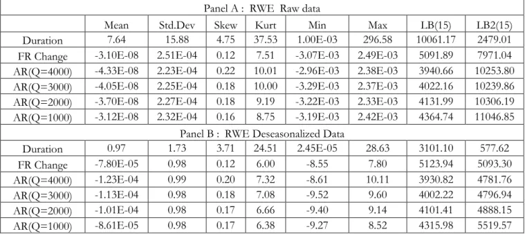
It is well known that high-frequency data behave very differently from low-frequency data. Table 1 presents the descriptive statistics of raw and deseasonalized duration, frictionless return changes and actual return changes for which various volumes are chosen for the three studied stocks. From Panel A, we can observe that for the entire sample period (July 2010), SAP is the most liquid stock as the average duration is the shortest and the number of observations is the largest. MRK is the least liquid one. Moreover, as the variables are constructed on tick-by-tick frequency, all three stocks have an average of zero and a very small standard deviation for frictionless return changes and actual return changes. All three stocks present high kurtosis due to the fact that most of the observations are concentrated on their average and co-exist with some extreme values. In addition, the raw data are also characterized by extremely high autocorrelation for both first and second moments for all of the variables.
High-frequency data are characterized by seasonality, which should be cleaned out before estimating any model. To do so, several approaches have been proposed in the literature: Andersen and Bollerslev (1997) use Fourier Flexible Functional (FFF) form to take off seasonality, Dufour and Engle (2000) remove seasonality by applying a simple linear regression with a dummy, and Bauwens and Giot (2000) take off seasonality by averaging over a moving window and linear interpolation.
[Insert Table 1 here]
However, as found in Anatolyev and Shakin (2007) and Dionne, Duchesne and Pacurar (2009), the high-frequency data could behave differently throughout the day as well as between different trading days. Therefore, in order to fully account
for the deterministic part exhibited in data, we apply a two-step deseasonalisation procedure, interday and intraday. Besides, it should also be noted that there exists an open auction effect in our continuous trading dataset similar to the one mentioned by Engle and Russell (1998). More precisely, for each trading day, the continuous trading follows the open auction in which specialists set a price in order to maximize the volume. Once the open auction is finished, the transactions are recorded. Consequently, the beginning of continuous trading is contaminated by extremely short durations. In addition, these short durations could produce negative seasonality factors of duration that are based on previous observations and cubic splines. To address this problem, the data for the first half hour are only used to compute the seasonality factor and then discarded.
The interday trend is extracted under a multiplicative form: , i s i,inter s dur dur dur = , , 2 ( ) f i s f i,inter f s r r r = , , 2 (15) ( ) b i s b i,inter b s r r r = where duri s, , , f i s r , , b i s
r are the ith duration, frictionless and actual return change for
day s, respectively and durs, 2
(rsf) , (rsb)2 are the daily average for day s for duration,
squared frictionless, and actual return changes, respectively.
Based on inter-day deseasonalized data, the intra-day seasonality is removed by following Engle and Russell (1998):
, , , 2 , 2 1 1 1 , , (16) ( ) (( ) ) (( ) ) f b i inter i inter i,inter f b
i intra i,intra f i intra b
i,inter i i,inter i i,inter i
r r
dur
dur r r
E dur I− E r I− E r I−
= = =
where E dur( i,inter) , E r(( i,interf 2) and E r((i,interb ) )2 are the corresponding deseasonality
factors constructed by averaging the variables over 30-minute intervals for each day of the week and then applying cubic splines to smooth these 30-minute averages. The same day of week shares the same intra-deseasonality curve.
However, it takes different deseasonality factors according to the moment of
transaction. Figure 1 illustrates the evolution of the seasonality factors of RWE for
duration, frictionless, and actual return changes when v = 4000.7 It is not surprising
to see that the frictionless and actual return changes have similar dynamics for the reason that the actual return changes contain the frictionless return changes. However, the magnitude is different for frictionless and actual return changes.
Panel B of Tables 1.1, 1.2 and 1.3 report descriptive statistics of deseasonalized
durations, frictionless and actual return changes. The raw frictionless and actual return changes have been normalized to have the mean equal to zero and standard deviation equal to one. However, other statistics such as skewness, kurtosis and auto-correlation are not affected by this normalization process. The high kurtosis and auto-correlation will be captured by the proposed models.
[Insert Figure 1 here] 6.2 Estimation results
We use the model presented in Section 5 to fit SAP, RWE and MRK deseasonalized data. The data cover the first week of July 2010. The data from the second week are used as out-of-sample data to test the model’s performance. As previously mentioned, the estimation is realized jointly for frictionless and actual return changes. The likelihood function is maximized using Matlab v7.6.0 with Optimization toolbox.
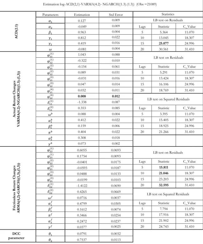
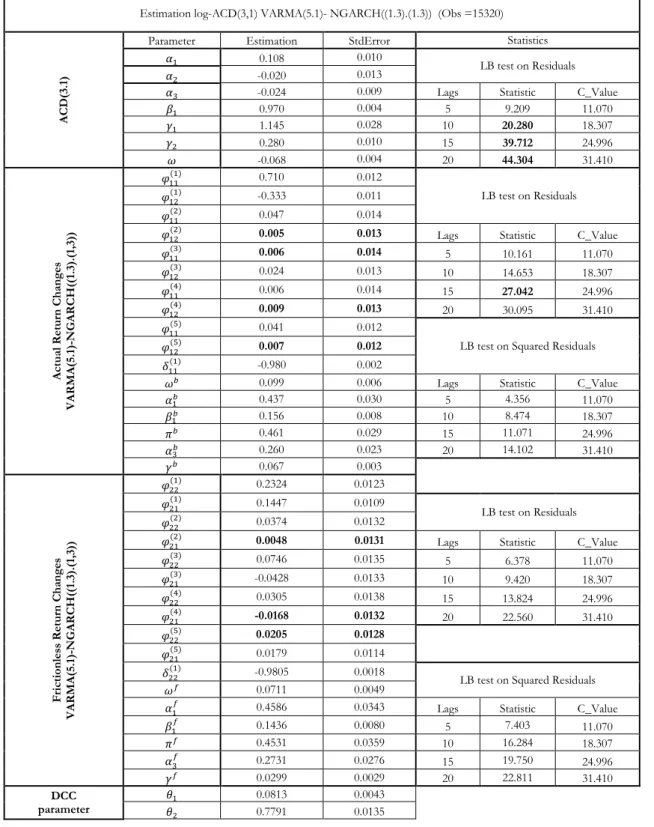
Tables 2.1, 2.2 and 2.3 report the estimation results for actual return changes for
SAP, RWE and MRK for v = 4000, 4000 and 1800 shares, respectively. It should
be noted that for each stock, the frictionless return changes and actual return changes are governed by the same duration process, which is assumed to be strictly exogenous. The high clustering phenomenon is indicated in deseasonalized data by the Ljung-Box statistic (see Table 1, Panel B). Furthermore, the clustering in duration is confirmed by the Log-ACD model. To better fit the data, we retain a
log-ACD (2,1) specification for SAP durations, a Log-ACD(3,1) model for RWE durations and a log-ACD(1,1) model for MRK durations. The Ljung-Box statistic on standardized residuals of duration provides the evidence that the Log-ACD model is capable of removing the high autocorrelation identified in deseasonalized duration data. The Ljung-Box statistic with 15 lags is dramatically reduced to 25.08 for SAP, to 39.7 for RWE and to 21.79 for MRK.
Frictionless and actual return changes of the three stocks are also characterized by a high autocorrelation in level and volatility. Moreover, the Ljung-Box statistics with 15 lags on deseasonalized return change and its volatility reject the independence at any significance level for the three stocks. Taking the model efficiency and parsimony into consideration, a
VARMA(4,2)-MGARCH((1,3),(1,3)))) 8 model is retained for SAP, a
VARMA(5,1)-MGARCH((1,3),(1,3)) model for RWE, and the specification of VARMA(2,2)-MGARCH((1,3),(1,3)) for MRK. The model adequacy is assessed based on standardized residuals and squared standardized residuals. Taking MRK as an example, the Ljung-Box statistics for standardized residuals and squared standardized residuals of actual return changes computed with 5, 15, 15, 20 lags, respectively, are not significant at the 5% level. The Ljung-Box statistic with 15 lags has been significantly reduced after modeling to 7.72. Similar results are obtained for stocks RWE and SAP.
Regarding the estimated parameters, the sum of coefficients in each individual GARCH model is close to one, indicating a high persistence in volatility.
Furthermore, non-zero of πf and πb in both structures provides the evidence of
asymmetry, that is, a negative shock generates a higher conditional volatility for the
next moment. It also should be noted that γb and γf are both positive for the
three stocks. This means that a longer duration will generate a higher volatility for both actual return and frictionless return changes. In addition, due to the fractional
exponent, the volatility increases with a decreasing speed when duration becomes longer. It should be noted that in our model the volatility is the product of
no-duration scaled variance and duration factor, and the γb of actual return
changes are higher than γf of frictionless return changes for the three stocks. This
implies that the duration factor has a larger impact on actual returns than frictionless returns.
The use of dynamic conditional correlation is justified by the fact that θ1 and θ2 in
equation (12) are both significantly different from zero for the three stocks. As expected, the conditional correlation of actual return and frictionless return changes is time-varying. The sum of two parameters around 0.8 confirms the high persistence of conditional correlation.
[Insert Table 2 here] 6.3 Model performance and backtesting
In this section, we present the simulation procedure and backtesting results on simulated deseasonalized and re-seasonalized frictionless and actual return changes. Once the model is estimated on tick-by-tick frequency, we can test the model
performance and compute frictionless IVaRc and LIVaRc by Monte Carlo
simulation. One of the advantages of our method is that once the model is
estimated, we can compute the simulated deseasonalized IVaRc and LIVaRc for any
horizon without re-estimating the model. In addition, we can compute the
simulation-based re-seasonalized IVaRc and LIVaRc in traditional calendar time
using the available seasonal factors.
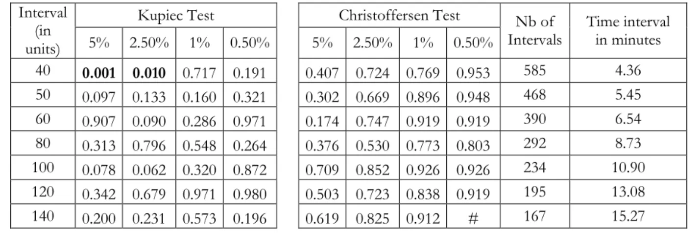
We choose different time intervals to test the model performance. The interval lengths are: 40, 50, 60, 80, 100, 120 and 140 units of time for more liquid stocks SAP and RWE and 20, 30, 40, 50, 60, 80 and 100 for less liquid stock MRK. As the model is applied to deseasonalized data, the simulated duration is not in calendar units. However, they are related in a proportional way. It should also be noticed
that, according to the trading intensity, the simulated duration does not correspond to the same calendar time interval. For a more liquid stock, the same simulated interval relates to a shorter calendar time interval. For instance, in the case of MRK, the interval-length 50 re-samples the one-week data for 190 intervals and corresponds to 13.42 minutes and the 100 interval-length relates to 95 intervals and corresponds to 26.84 minutes. However, for a more liquid stock such as SAP, 50 interval-length corresponds to 5.45 minutes and 140-interval-length to 15.27 minutes.
The simulations for frictionless and actual return changes are realized as follows: 1) We generate the duration between two consecutive transactions since we assume that the duration process is strongly exogenous.
2) With the simulated duration and estimated coefficients of the VARMA-NGARCH model, we obtain the corresponding return changes.
3) We repeat steps 1 and 2 for 10,000 paths and re-sample the data at each path according to the predetermined interval.
4) For each interval, we compute the corresponding IVaRc and LIVaRc at the
desired level of confidence. To conduct the backtesting for each given interval, we also need to construct the return changes for original out-of-sample data.
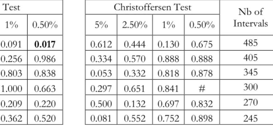
To validate the model, we conduct the Unconditional Coverage and Independence tests by applying Kupiec test (1995) and Christoffersen test (1998). The Kupiec test checks whether the empirical failure rate is statistically different from the failure rate we are testing, whereas the Christoffersen test aims at evaluating the independence aspect of the violations. More specifically, it rejects VaR models that generate clustered violations by estimating a first order Markov chain model on the sequence. Table 3 reports the p-values for the Kupiec and the Christoffersen tests upon simulated data for confidence levels of 95%, 97.5%, 99% and 99.5%. The time interval varies from 5 minutes to 15 minutes for SAP, from 5 minutes to
16.67 minutes for RWE and from 5 minutes to 27 minutes for MRK. Most of p-values are higher than 5% indicating that, in general, the model captures well the distribution of frictionless and actual return changes.
[Insert Table 3 here]
Since most of trading and risk management decisions are based on the calendar time and raw data, it might be difficult for practitioners to use simulated deseasonalized data to conduct risk management. To this end, we conduct another Monte Carlo simulation that takes into account the time-varying deterministic seasonality factors. The process is similar to that used for simulating deseasonalized data. However, the difference is that we re-introduce the seasonality factors for duration, actual return changes and frictionless return changes. As seasonality factors vary from one day to another, the simulation should take the day of week into account. More precisely, for the first day, simulated durations are converted to a calendar time of that day and then the corresponding timestamp will identify the seasonality factors for actual and frictionless return changes. The simulation process will continue until the corresponding timestamp surpasses the closing time for the underlying day. In the case of a multiple-day simulation, the processes will continue for another day. Based on the simulated re-seasonalized
data, we also compute our IVaRc and LIVaRc by repeating the same algorithm.
Table 4 presents the backtesting results on the re-seasonalized simulated data. The time interval varies from 5 minutes to 10 minutes for the three stocks and the confidence levels to test are 95%, 97.5%, 99% and 99.5%. Similar to the test results for simulated deseasonalized data, both the Unconditional Coverage test and Independence test suggest that the simulated re-seasonalized data can also provide reliable high-frequency risk measures for all chosen confidence levels over intervals from 5 to 10 minutes.
7 Risks for Waiting Cost, Ex-ante Liquidity Risk and Various IVaRs 7.1 Risks for waiting cost
As shown in Section 4, the sums of tick-by-tick frictionless return changes and actual return changes over a given interval can be viewed as the waiting costs related to market risk and total risk, which contains market risk and ex-ante
liquidity risk. Consequently, the corresponding IVaRc and LIVaRc estimate the risk
of losses on these waiting costs. Based on simulated re-seasonalized data from previous section that contain the determinist (seasonal factor) and random (error term) elements, we can further investigate the effect of the ex-ante liquidity risk embedded in the open LOB on the total risk. To this end, we define an impact
coefficient of ex-ante liquidity risk9:
𝛤𝑖𝑛𝑡,𝑣 = 𝐿𝐼𝑉𝑎𝑅𝚤𝑛𝑡,𝑣 𝑐 � − 𝐼𝑉𝑎𝑅�𝚤𝑛𝑡𝑐 𝐿𝐼𝑉𝑎𝑅�𝚤𝑛𝑡,𝑣𝑐 (17) As mentioned above, c int,t IVaR and c int,v,t
LIVaR are the VaRs for frictionless return
changes and actual return changes of volume v for the t-th interval. As we simulate
the data in the tick-by-tick framework, we can compute the c
int,t
IVaR and c
int,v,t LIVaR
for any desired interval. Accordingly, 𝐼𝑉𝑎𝑅� 𝚤𝑛𝑡𝑐 and 𝐿𝐼𝑉𝑎𝑅�𝚤𝑛𝑡,𝑣𝑐 are the averages of
c int,t
IVaR and c
int,v,t
LIVaR . As a result, Γint,v assesses, on average, the impact of the
ex-ante liquidity risk of volume v on total risk for a given interval. Figure 2 shows
how the impact coefficients of ex-ante liquidity perform for intervals from 3 minutes to 10 minutes for the three stocks.
[Insert Figure 2 here]
There are two interesting points to stress after observing the plots. First, the curve is globally increasing, that is, in most of the times, the impact coefficient of the ex-ante liquidity increases when interval increases and will finally converge to its
9 The risk measures in equation (17) are computed for confidence level 95%; in practice, other confidence levels can
run level. It should be noted that the relation of frictionless return changes and
actual return changes can be explicitly expressed by rib =rif +riLOB,where
LOB i
r is the
volume-dependent LOB return change for i-th transaction. Econometrically, as the
sum of two ARMA structures is also an ARMA structure (Engel (1984)), the difference of the frictionless return changes and the actual return changes follow
implicitly another ARMA structure. Accordingly, the relationship of c
int,t
IVaR and
c int,v,t
LIVaR can be generally written as:
int, (18)
c c c F,LOB
int,v,t t int,v,t int,v,t
LIVaR = IVaR +LOBIVaR +Dep
c int,v,t
LOBIVaR measures the risk associated with the open LOB and F,LOB
int,v,t
Dep presents
the dependence between the frictionless return changes and the actual return changes, which can stand for various dependence measures. However, in our
specific modeling, F,LOB
int,v,t
Dep is the covariance between rif and riLOB. Therefore, the
numerator of equation (17) is the sum of c
int,v,t
LOBIVaR and Depint,v,tF,LOB. The fact that the curve is globally increasing in time is due to the higher autocorrelation in LOB return changes over time, which are the changes of magnitude in LOB caused by a given ex-ante volume.
The convergence means that, for the long run, the sum of c
int,v,t
LOBIVaR and Depint,v,tF,LOB
is proportional to c
int,v,t
LIVaR . Recall that in a general GARCH framework, the
forward multi-step volatility will converge to its unconditional level. In the present study, once the intervals include sufficient ticks for which the volatilities of both LOB return changes and frictionless return changes reach their unconditional levels, the volatilities of the sum of both return changes will increase with the same speed and therefore the impact coefficient of the ex-ante liquidity will converge to its asymptotic level.
Second, it is interesting to observe that the impact coefficients of ex-ante liquidity of RWE stock are negative for a volume of 1000 shares and become positive when
volumes are 2000, 3000 and 4000 shares. A negative impact coefficient of ex-ante liquidity indicates that volatility for the actual return changes is less than that of the frictionless return changes. In other words, the ex-ante liquidity risk embedded in LOB offsets the market risk. This again results from the fact that off-best levels of LOB are more stable than first level. Based on equation (18), when the volume is small, the negative correlation between frictionless return change and LOB return change plays a more important role in determining the sign of the impact coefficients of ex-ante liquidity. However, for a higher ex-ante volume, the risk of LOB return change also increases but faster than its interaction with frictionless return change. Consequently, the impact coefficients of ex-ante liquidity become positive.
7.2 High-frequency ex-ante liquidity premium
Based on the tick-by-tick simulation, we can also compute the high-frequency
IVaRand LIVaR for frictionless return and actual return. Using IVaRand LIVaR
of the same stock, we can further define a relative interval-dependent liquidity premium as follows: (19) int,v,t int,t int,v,t int,v,t LIVaR IVaR LIVaR − Λ =
Similar to the liquidity ratio proposed in Giot and Grammig (2006), IVaRint,t and
int,v,t
LIVaR are the VaR measures for frictionless return and actual return at the end
of t-th interval and int is the predetermined interval such as 5-min, 10-min, etc. It
should be noticed that our defined actual return and frictionless return do not have the time-additivity property but the frictionless return changes and actual return changes do. Even though the VaR based on frictionless return changes and actual return changes can be used directly in practice, in some situations, practitioners might want to predict their potential loss on frictionless return or actual return instead of frictionless and actual return changes for a precise calendar time point.
To illustrate how our model can be used to provide the ex-ante risk measure for frictionless return and actual return, we first compute the return changes for frictionless returns and actual returns, then calculate the instantaneous frictionless return and actual return at the beginning of the given interval using equations (3) and (4). Once we know the frictionless return and actual return at the beginning of a given interval, we can obtain the frictionless return and actual return for the end of the interval. Figure 3 illustrates how the frictionless return and actual return at the end of an interval are computed. Figure 4 then illustrates the evolutions of IVaR and LIVaR associated with a large liquidation volume for SAP, RWE and
MRK during one out-of-sample day, July 12th, 2010. For the three stocks, the IVaR
and LIVaR both present an inverse U shape during the trading day. However, for the more liquid stock SAP, the IVaR and LIVaR are less volatile than those of the less liquid stocks RWE and MRK. It also seems that the total risk is smaller during the middle of day. Nonetheless, it should be noted that the smaller VaR in absolute terms does not mean we should necessarily trade at that moment. The IVaR and LIVaR only provide the estimates of potential loss for a given probability at a precise point in time.
[Insert Figure 3 here] [Insert Figure 4 here]
In addition, the difference between curves on each graph, which measures the risk associated with ex-ante liquidity, varies with time. This is due to the fact that LOB interacts with trades and also changes during the trading days. Smaller (bigger) difference indicates a deeper (shallower) LOB. More specifically, for the least liquid stock, MRK, the ex-ante liquidity risk is more pronounced even for a relatively smaller quantity of 1800 shares. Regarding the more liquid stocks such as SAP and RWE, the ex-ante liquidity risk premiums are much smaller even for the relatively larger quantities of 4000 shares. This again suggests that the ex-ante liquidity risk
becomes more severe when the liquidation quantity is large and the stock is less liquid.
7.3 Comparison of LIVaR and other intraday VaRs
Our proposed IVaR and LIVaR, which are validated by backtesting, allow us to conduct more analysis on ex-ante liquidity and compare them with other high-frequency risk measures in existing literature.
The standard IVaR proposed by Dionne, Duchesne and Pacurar (2009) is based on a transaction price that is similar to the closing price in daily VaR computation. However, the resulting IVaR serves as a measure of potential loss of ‘paper value’ for a frozen portfolio and it omits the ex-ante liquidity dimension. To some extent, the IVaR accounts for an ex-post liquidity dimension; more specifically, it measures the liquidity already consumed by the market. However, active traders are more concerned with ex-ante liquidity because it is related to their liquidation value. For any trader, the risk related to liquidity is always present and the omission of this liquidity dimension can cause a serious distortion from the observed transaction price especially when the liquidation volume is large.
Another major difference is that before obtaining LIVaR, we should compute
LIVaRc for actual return changes, which gives the potential loss in terms of waiting
costs over a predetermined interval. Accordingly, the resulting LIVaRprovides a
risk measure for actual return at a given point in time while the standard IVaR is based on tick-by-tick log-returns, which have time-additive property. It thus directly gives a risk measure in terms of price for a given interval.
The high-frequency VaR proposed by Giot and Grammig (2006) is constructed on mid-quote price and ex-ante liquidation price over an interval of 10 or 30 minutes. The mid-quote price is usually considered as the efficient market price in market microstructure theory. However, from a practical perspective, the traders can rarely obtain the quote price during their transactions. Therefore, the use of
mid-quote price will underestimate the risk faced by high-frequency traders. Instead of taking the mid-quote price as the frictionless benchmark, we take a more realistic price, best bid price, as the frictionless price for traders who aim at liquidating their stock. Consequently, for active day-traders, our LIVaR can be considered an upper
bond of risk measure that provides the maximum p-th quantile in absolute value
when liquidating a given volume v. Figure 5 illustrates the difference in
constructing the frictionless returns and actual returns. [Insert Figure 5 here] 8. Conclusion
In this paper, we introduce the ex-ante liquidity dimension in an intraday VaR measure using tick-by-tick data. In order to take the ex-ante liquidity into account, we first reconstruct the LOB for three blue chip stocks actively traded in Deutsche Börse (SAP, RWE and MRK) and then define the tick-by-tick actual return that is the log ratio of ex-ante liquidation price computed from a predetermined volume
over the previous best ask price. Correspondingly, the proposed IVaRc and LIVaRc
are based on the frictionless return changes and actual return changes and relate to the ex-ante loss in terms of actual return. In other words, both risk measures can be considered as the waiting costs associated with market risk and liquidity risk. In order to model the dynamic of actual return, we use a logACD-VARMA-MGARCH structure that allows for both the irregularly spaced durations between two consecutive transactions and stylized facts in changes of actual return. In this setup, the time dimension is supposed to be strongly exogenous. Once the model is estimated, Monte Carlo simulations are used to make multiple-steps forecasts. More specifically, the log-ACD process generates first the tick-by-tick duration while the VARMA-MGARCH simulates the corresponding conditional tick-by-tick frictionless return changes and actual return changes. The model performance is assessed by using the tests of Kupiec (1995) and Christoffersen (1998) on both simulated deseasonalized and re-seasonalized data. Both tests indicate that our
model can correctly capture the dynamics of frictionless returns and actual returns over various time intervals for confidence levels of 95%, 97.5%, 99% and 99.5%. Our LIVaR provides a reliable measure of total risk for short horizons. In addition, the simulated data from our model can be easily converted to data in the calendar time. Practically, the potential users of our measure could be the high-frequency traders that need to specify and update their trading strategies within a trading day or the market regulators who aim to track the evolution of market liquidity, and the brokers and clearing houses that need to update their clients’ intraday margins. Future research can continue in several directions. Our study is focused on a single stock ex-ante liquidity risk. A possible alternative is to investigate how the IVaR and LIVaR evolve in the case of a portfolio. In particular, the no-synchronization of the durations between two consecutive transactions for each stock is a challenge. Another direction is to test the role of ex-ante liquidity in different regimes. Our study focuses on the liquidity risk premium in a relatively stable period. It could also be interesting to investigate how the liquidity risk behaves during a crisis period. This study will require a more complicated econometric model to take into account different regimes.