HAL Id: hal-00707750
https://hal.archives-ouvertes.fr/hal-00707750
Submitted on 8 Oct 2020HAL is a multi-disciplinary open access archive for the deposit and dissemination of sci-entific research documents, whether they are pub-lished or not. The documents may come from teaching and research institutions in France or abroad, or from public or private research centers.
L’archive ouverte pluridisciplinaire HAL, est destinée au dépôt et à la diffusion de documents scientifiques de niveau recherche, publiés ou non, émanant des établissements d’enseignement et de recherche français ou étrangers, des laboratoires publics ou privés.
Distributed under a Creative Commons Attribution| 4.0 International License
Route to chaos in a circuit modeled by a 1-dimensional
piecewise linear map
Danièle Fournier-Prunaret, Pascal Charge
To cite this version:
Danièle Fournier-Prunaret, Pascal Charge. Route to chaos in a circuit modeled by a 1-dimensional piecewise linear map. Nonlinear Theory and Its Applications, IEICE, The Institute of Electronics, Information and Communication Engineers, 2012, 3 (4), pp.521-532. �10.1587/nolta.3.521�. �hal-00707750�
Route
to chaos in a circuit modeled by a
1-dimensional
piecewise linear map
Dani`
ele Fournier-Prunaret
1a)and Pascal Charg´
e
2b)1 INSA, Universit´e de Toulouse
LAAS-CNRS, 7 avenue du colonel Roche, F-31077 Toulouse Cedex 4, France
2 Lunam University, University of Nantes
UMR CNRS 6164 IETR, Polytech Nantes, France
a)[email protected] b)[email protected]
Abstract: A very simple hybrid circuit proposed as chaos generator is studied. It is modeled using a 3-slopes piecewise linear map defined on [0,1] and depending upon three parameters. The parameter space is investigated in order to classify regions of existence of stable periodic orbits and regions associated with chaotic behaviors. Bifurcation curves are obtained numer-ically and analytnumer-ically. Border collision bifurcations and homoclinic bifurcations occurring in cyclical chaotic regions leading to chaos in one-piece are detected.
Key Words: piecewise linear bimodal map, chaos generator, border collision bifurcation
1. Introduction
Many circuits including switches have been considered during the last decade. Such systems are of interest for two reasons: first, they belong to the class of hybrid systems that have attracted much interest those last ten years, secondly, they permit to obtain chaos in a very easy way. Hybrid systems have been much considered in many kinds of applications during the last decade. Such systems appear for example in Electronics and Electrotechnics and the understanding of their behaviour is of great interest. Hybrid systems evolve in continuous time, but it is possible to model them using discrete time maps, by introducing a discretization similar to the building of a Poincar´e map. This is the case for the circuit we consider in this paper. Concerning the second point, chaotic signals have appeared as very useful in many kinds of applications in the last twenty years, particularly in telecommunications and image processing. Indeed, for some kind of applications, it is necessary to consider robust chaos [1], which can endure, even if parameter values are slightly modified. A way to obtain robust chaotic signals is to consider systems where border collision bifurcations appear [2, 3, 6, 8, 9], that generally constitute a class of hybrid systems. Chaotic generators can also be obtained using continuous time models as systems based on the Chua’s circuit (analogical circuit), while others are discrete time systems which directly iterate a chaotic map (digital circuit). The problem with these systems is that chaos is not necessarily as robust.
managed using a clock (impulse waveform) and the charging/discharging of the capacitor. We have previously proposed such a kind of chaos generator, where the model was a two-dimensional nonlinear map [4, 5, 10]. Our aim in considering a one-dimensional case is to analyze rigorously the bifurcations and to prove the existence of chaos in an even more simple circuit.
The section 2 is devoted to the description of the circuit and its modeling. The model under a one-dimensional piecewise linear map is given in section 3. The dynamical behaviour of the map, with the study of bifurcations permitting to obtain periodic orbits and chaos is explained for some parameter values in section 4.
2. Description of the circuit
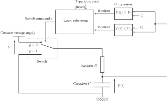
The 1D proposed chaos generator is a quite simple circuit given in Fig. 1, very similar to those discussed in [3, 6]. The analog state variable is V (t), the voltage across the capacitor. We can see that the switch position is ruled by the logic subsystem output p. In the same time inputs of the logic subsystem are provided by comparison of the analog state variable V (t) with constant voltages VU
and VD. Analog and logic subsystems then form a hybrid system.
Fig. 1. The hybrid circuit including the analog and logic subsystems.
Behavior of the logic subsystem can be described by the following finite state diagram. At any state transition, the condition is given by the boolean expression above the line, whereas the action at the transition is indicated below the same line. As an example, the transition from the state C1 to the
state D occurs when the expression ((t < T ) & (V (t) ≥ VU)) is true. At this transition instant, the
system output p is set to the logic value 1. Actions are then described with variables allocations. The variable t denotes the time. When the time reaches the value t = T , a state transition is expected and the time variable is reset (allocation t := 0;).
From this diagram observation, it comes that the logic subsystem is an asynchronous sequential system, that is periodically forced to return to the state C1 by an external periodic event. In [11, 15],
we proposed a very simple implementation of this logic subsystem based on a few R-S latches and logic operators. The periodic event is then realized thanks to a pulse generator.
A switch occurs at every T -periodic event or when the state variable V (t) reaches the value of VD
or VU. The capacitor charges (p=0) when V (t) reaches VD or discharges (p=1) when V (t) reaches
VU. Let us call V the reference voltage, VA the borderline value corresponding to V (t) = VU, VB
the borderline value corresponding to V (t) = VD and τ = RC. Let us call V the reference voltage,
Fig. 2. The finite state diagram, which describes the logic subsystem.
3. Modeling
By considering the classical equations of a RC circuit, we obtain VA = V − (V − VU)e
T
τ, VB =
V − VD
VU(V − VU)e T
τ. Let us call Vn, the state value at each time t = T when the time is initialized
again, we obtain the following relations:
0 < Vn≤VA , Vn+1= V − (V − Vn)e− T τ VA< Vn< VB , Vn+1= (V − Vn)V −VVUUe− T τ VB < Vn≤1 , Vn+1= V − (V − Vn)VVUDV −VV −VDUe− T τ (1)
We normalize the state variables and the parameters in order to deal with dimensionless values and a normalized phase space equal to [0, 1]:
xn= VVn ∈[0, 1] , xn+1= Vn+1V ∈[0, 1] β= VU V ∈]0, 1[ , 0 < m = VD VU <1 , δ = e −Tτ ∈]0, 1] xb= VVB, xa= VVA (2)
The following switching values in [0, 1] are:
xa= 1 −1−βδ
xb = 1 −m(1−β)δ
(3)
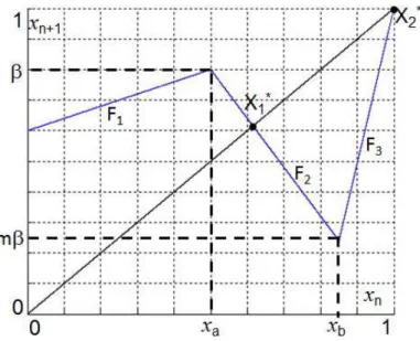
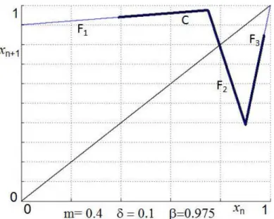
Finally, the circuit is modeled by the map xn+1= F (xn) (cf. Fig. 3), which is defined as follows:
if xn∈[0, xa[, F (xn) = F1(xn) = 1 − (1 − xn)δ
if xn∈[xa, xb[, F(xn) = F2(xn) = (1 − xn)1−βδβ
if xn∈[xb,1], F (xn) = F3(xn) = 1 − (1 − xn)mδ 1−βm1−β
(4)
It is easy to see that the map is well defined as F is continuous and maps the interval [0, 1] (the phase space of interest) into itself.
Fig. 3. The 3-pieces piecewise linear map.
4. Dynamical behaviour of the 1-D model
The map (4) is a 1-dimensional piecewise linear map with three pieces. In this section, we study the fixed points, order k periodic orbits and their bifurcations. We also put in evidence the homoclinic bifurcations giving rise to chaotic behaviour. First, let us give the slopes of the map, depending where is located the point in the interval [0, 1]. These values will be useful for the rest of our study.
if x ∈[0, xa[, p1= δ > 0
if x ∈[xa, xb[, p2= −δβ1−β <0
if x ∈[xb,1], p3= mδ 1−βm1−β >0
(5)
4.1 Bifurcations of fixed points and order 2 periodic orbits
This study has been previously done in [4, 15]. We recall the results. Two fixed points X∗
1 and X2∗
exist and are given by:
X∗ 1 = 1−β+δβδβ ∈[xa, xb] X∗ 2 = 1 (6) X∗
1 is stable when the slope p2= −δβ1−β ∈] − 1, 0[, that means β < 1+δ1 . X2∗ is stable when the slope
p3 = mδ 1−βm1−β ∈]0, 1[, that means β < mm−δ(1−δ) and m > δ. So, we can define the bifurcation curves
related to fixed points bifurcations:
F B1a : β = 1+δ1 , m < δ, F B1b : β = 1+δ1 , m > δ F B1c : β = m−δ
m(1−δ), m > δ
(7)
These curves correspond to degenerate flip bifurcations, F B1a corresponds to the appearance of a stable order 2 cycle after the flip bifurcation of X∗
1, F B1b corresponds to the appearance of an
order 2 cyclic chaotic attractor (C1, C2), after X1∗ has changed its stability (see Fig. 6); for instance,
the order 2 periodic orbit (Y1, Y2), which appears at the flip bifurcation F B1b, undergoes in the
same time a border collision bifurcation (Y2 is merging with xb) and becomes unstable (see Fig. 5).
F B1c corresponds to a border collision bifurcation for X∗
1, which disappears when merging with xb
(β below F B1b in the plane (m, β), δ being fixed); at the same bifurcation value, X∗
2 becomes a
stable fixed point (β below F B1b in the plane (m, β), δ being fixed). The curve F B1c (β above F B1b) also corresponds to a degenerate bifurcation for X∗
2 with the appearance of an order 2 cyclic
chaotic attractor, after X∗
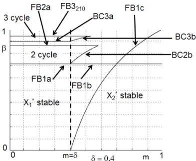
Fig. 4. In the (m, β) plane, δ = 0.4, bifurcation curves of the map F related to fixed points and order 2 and 3 cycles.
Fig. 5. Degenerate flip bifurcation (F B1b) in the plane (xn, xn+1) for δ = 0.4,
m= 0.6 and β = 0.7142857.
homoclinic bifurcation, gives rise to an one-piece chaotic attractor (see Fig. 7). Such chaos can be considered as robust in the sense of remaining chaotic even if the parameters or the initial conditions are slightly changed [1].
When there exists a stable order 2 cycle, this cycle can undergo a degenerate flip bifurcation, which gives rise to an order 4 cyclic chaotic attractor. The bifurcation curve is given by the following equation, corresponding to the slope of F2 that becomes equal to −1 (see Fig. 4):
F B2a : β =1+δ12 (8)
F B2a corresponds to the slope of F2 equal to p
1p2 (F2 = F1F2). It is impossible to obtain a flip
bifurcation for F2= F
1F3, because p1p3 can never be negative.
Other bifurcation curves correspond to border collision bifurcations. It is possible to have F2(x a) =
xa or F2(xb) = xb. The corresponding curves are respectively denoted BC2a and BC2b. Their
equations are given by:
BC2a : β = 1+δ1 BC2b : β = m−δ2
m(1−δ2), m > δ2
Fig. 6. An order 2 cyclic chaotic attractor (C1, C2) exists for δ = 0.4, m = 0.6
and β = 0.75. Let us remark that we have plotted the chaotic attractor in the plane (xn, xn+1) for a better visualization.
Fig. 7. An one-piece chaotic attractor C appears after an homoclinic bifur-cation. Parameter values are δ = 0.4, m = 0.6 and β = 0.8.
Let us remark that BC2a = F B1b. The bifurcation curves related to fixed points and order 2 cycles are plotted on Fig. 4.
4.2 Bifurcations of order k periodic orbits
Using the same method as for fixed points and order 2 cycles, we can obtain the bifurcation curves for order k cycles. In this paragraph, we do not intend to study and write the bifurcation curves equations for all the categories of order k cycles that can be defined, but only for those that we have obtained in numerical simulations. Previous studies concerning bimodal piecewise linear maps have been done in a more general way [7, 12]. In this work, we only intend to give the analytical forms of bifurcation curves equations with the aim of a practical use for our model.
First, we give the bifurcation curves corresponding to the degenerate flip bifurcations. Indeed, if we consider an order k cycle, each point X of this cycle verifies Fk(X) = X and Fk is obtained by
a combination of its three determinations F1, F2 and F3. We can write that, in Fk, F1 appears i
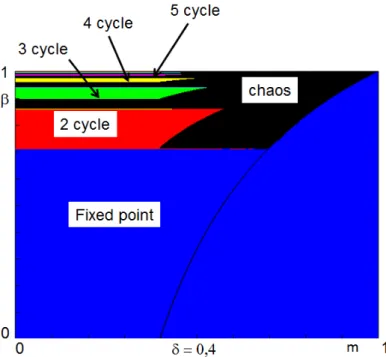
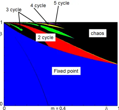
Fig. 8. Stability areas of k periodic orbits in the parameter plane (m, β) for δ= 0.4. They are limited by bifurcation curves obtained in Fig. 4.
obtained by considering the three slopes p1, p2 and p3 such that pi1p j
2pl3= −1. This curve is denoted
F Bkijl and is given by the following equation:
F Bkijl: δi(β−1δβ )j(mδ 1−βm1−β )l= −1, i + j + l = k, (10)
which can also be written:
δk= (1−β)(1−βm)j+llmβjl, i+ j + l = k (11)
All the degenerate flip bifurcation curves are known analytically and can be plotted in the parameter planes (β, δ), m being fixed or (m, δ), β being fixed.
It is also possible to find the border collision bifurcation curves. The collision can occur with any of both points xa or xb. So, we will have to look the parameter values for which one has Fk(xa) = xa
or Fk(x
b) = xb. Anyhow, we have to look at the way of exchanging the points of cycles by F .
The simplest case occurs when an order k cycle has its points exchanged k − 1 times by F1 and
one time by F2 or k − 1 times by F1 and one time by F3. It is possible to obtain the border collision
bifurcation curves, which are denoted BCka if the collision occurs with xa, that means Fk(xa) = xa,
or BCkb if the collision occurs with xb, that means Fk(xb) = xb. The corresponding equations are:
BCka: β = 1−δ1−δk−1k , m < δ
BCkb: β = m−δ2
m(1−δ2), m > δ2
(12)
On Fig. 4 are plotted the bifurcation curves of an order 3 cycle whose exchange of points is given by F2
1F2. Figure 8 gives the areas of stability of order k periodic orbits, k = 1, ...5, it is very easy to
observe that these areas are limited by the bifurcation curves obtained in Fig. 4. An enlargment of these figures is provided in Fig. 9 and Fig. 10, which permits to put in evidence order 6 and 7 cycles. Bifurcation curves of order k cycles, k = 1, ...7 are plotted on Fig. 10. All these cycles are cycles of Fk = Fk−1
1 F2. Let us remark that we obtain a period-adding sequences of periodic orbits. Between
two stability areas of periodic orbits, chaos appears (k-pieces chaotic attractor), which undergoes a succession of homoclinic bifurcations giving rise to an one-piece chaotic attractor.
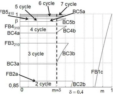
On Fig. 8, we consider the parameter plane (δ, β), m being fixed and equal to 0.4, we can see the stability areas of some order k cycles, k = 1, ...5. On Fig. 12 and Fig. 13, an enlargment permits to obtain order k cycles, k = 1, ..., 7. Those cycles have their points exchanged as given below (we consider the cycles from left to right in the figures). It is also possible to use Symbolic Dynamics of a
Fig. 9. Enlargment of Fig. 8, order k cycles are observed, k = 1, ..., 7.
Fig. 10. Bifurcation curves corresponding to the limit of stability regions of Fig. 9 in the parameter plane (m, β) for δ = 0.4.
bimodal map [13, 14], we have chosen to represent a cycle by beginning with the point at the left of the interval [0, 1] (generally, this point is located inside I1 and F1 is applying). The use of symbolic
dynamics corresponds to give a code to every order k cycle by considering the location of the points in the intervals I1, I2 or I3; generally, the following rule is used: a point of the cycle is coded by L
when it belongs to I1, M when it belongs to I2 and R when it belongs to I3 (sometimes, the codes A
or B can be used if one point of the cycle is merging with xa or xb, in this paper, we will not take
this possibility into account). Here are the obtained coding for the cycles of Fig. 12 from left to right in the figure:
• order 6 cycle, F2F34F1, LRRRRM
• order 5 cycle, F2F33F1, LRRRM
• order 4 cycle, F2F32F1, LRRM
Fig. 11. Stability areas of k periodic orbits, k = 1, 2, 3 in the parameter plane (δ, β) for m = 0.4.
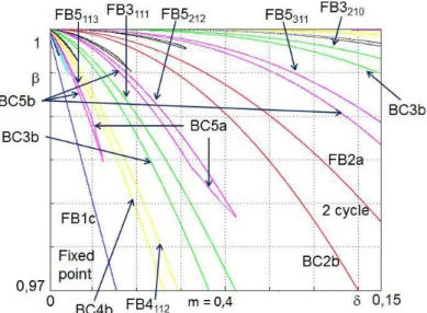
Fig. 12. Enlargment of Fig. 11. Stability areas of k periodic orbits, k = 1, ..., 7 in the parameter plane (δ, β) for m = 0.4. They are limited by bifurca-tion curves obtained in Fig. 13.
• order 3 cycle, F2F3F1, LRM • order 5 cycle, F2(F3F1)2, LRLRM • order 7 cycle, F2(F3F1)3, LRLRLRM • order 2 cycle, F2F1, LM • order 7 cycle, F1F2F1(F3F1)2, LRLRLM L • order 5 cycle, F1F2F1F3F1, LRLM L • order 3 cycle, F2F12, LLM
Fig. 13. Bifurcation curves of k periodic orbits, k = 1, 2, 3, 4, 5, 6, 7 in the parameter plane (δ, β) for m = 0.4. They limit the stability areas of Fig. 12. In order to clarify the figure, only bifurcation curves for k = 1, ..., 5 have been indicated.
• order 7 cycle, F2F12F3F13, LLLRLLM
• order 4 cycle, F2F13, LLLM
All the stability areas in Fig. 12 are bounded by degenerate flip bifurcation curves DF Bkijl (10)
or border collision bifurcation curves. The border collision bifurcation curves must be calculated by considering the exchange of the points of the cycle and the point xa or xb with which there is a
collision. The cycles above can be classified in different categories, related to the kind of symbols which represent them or regarding the way of exchanging their points. We can propose the following classification and give the equations of the border collision bifurcation curves for each of them (let us recall that the degenerate flip bifurcation curves are given by (10)(11)):
• The order 2 cycle (F2F1, LM ), the order 3 cycle (F2F12, LLM ) and the order 4 cycle (F2F13,
LLLM) have already been studied and their bifurcation curves are given in (10)(11)(12). • The order 6 cycle (F2F34F1, LRRRRM ), the order 5 cycle (F2F33F1, LRRRM ), the order 4
cycle (F2F32F1, LRRM ) and the order 3 cycle (F2F3F1, LRM ) belong to the same class of
order k cycle, which can be denoted: F2F3k−2F1, LR...RM , where the symbol R appears (k − 2)
times. The border collision bifurcation curves are given by:
BCka: δk(1−βm)δ(1−β)k−2β+(1−β)k−2mk−2k−1mk−2 = 1,
BCkb: δk= ((1−β)m (1−βm))k−1
(13)
• The order 5 cycle (F2(F3F1)2, LRLRM ) and the order 7 cycle (F2(F3F1)3, LRLRLRM ) belong
to the same category of order k cycle, k odd, which can be denoted: F2(F3F1)
(k−1)
2 , LRLR...M ,
where the symbol LR appears (k−1
2 ) times. The border collision bifurcation curves are given
by: BCka: δk−2(1−βm) k−3 2 mk−4(1−β)k−12 −δkβ(1−βm) k−1 2 mk−3(1−β)k+12 = 1, BCkb: δk= ((1−β)m (1−βm)) k+1 2 (14)
• Concerning the order 7 cycle (F2(F32F1)2, LRRLRRM ), we only give its own bifurcation curves:
BCka: −δ7mβ4(1−βm)(1−β)54 + δ4(1−βm)2 m2(1−β)3 = 1, BCkb: δ7= ((1−β)m (1−βm))5 (15)
Fig. 14. A chaotic attractor is located in the three intervals I1, I2 and I3
and is issued from an order 3-cycle whose points are exchanging using the three determinations of F .
• The order 7 cycle (F1F2F1(F3F1)2, LRLRLM L) and the order 5 cycle (F1F2F1F3F1, LRLM L)
belong to the same category of order k cycle, k odd, which can be written under the following general form: F1F2F1(F3F1)
(k−2)
3 , LRLR...LRLM L, where the symbol LR appears k−3
2 times.
The border collision bifurcation curves are given by:
BCka: (1−β)δ2 − δ k β(1−βm)k−32 mk−32 (1−β)k−12 = 1, BCkb: δk= ((1−β)m (1−βm))k−3 (16)
• Concerning the order 7 cycle (F2F12F3F13, LLLRLLM ), we only give its own bifurcation curves:
BCka: δ3 (1−β)− δ7β(1−βm) m(1−β)2 = 1, BCkb: δ7= ((1−β)m (1−βm))2 (17)
All the bifurcation curves for order k cycles, k = 1, ..., 7 are plotted on Fig. 13. They clearly limit the stability areas of order k cycles of Fig. 12. The curves of degenerate flip bifurcations and border collision with xb are given in an explicit form and can be directly plotted, the curves related to the
border collision with xaare given under an implicit form and have to be plotted by using a numerical
method (Newton-Raphson).
Between two stability regions, there exists a chaotic attractor. The chaotic attractor issued from a degenerate flip bifurcation is a cyclic one, then after a succession of homoclinic bifurcations, it becomes an one-piece chaotic one.
For some parameter values, chaos can be located on the three domains I1, I2and I3(Fig. 14). This
chaos is obtained from border collision bifurcations of order k-cycles whose points exchange by F1, F2
and F3. This is the case around the stability area of the order 3-cycle (F2F3F1, LRM )(see Fig. 12).
In this case, chaos can be considered as robust; indeed its existence domain in the parameter space is large enough.
5. Conclusions
We have proposed a very simple circuit under the form of a hybrid system, which presents two major interests. First, this circuit is modeled by a one-dimensional piecewise bimodal linear map, such map exhibits very rich signals properties and dynamics. Secondly, such a circuit allows to produce chaotic signals, which can be robust in the sense of remaining chaotic even if the parameters or the initial conditions are slightly changed; such chaotic signals can be very useful for different kinds of
applications. The model is very simple and depends on three parameters, we have been able to derive the exact analytical expressions of degenerate flip bifurcation and border collision bifurcation curves in the parameter space for some periodic orbits. The border collision bifurcations give rise to chaos, which can be robust, depending upon parameter values and configurations of periodic orbit sequences in parameter space. We intend to continue our study, in order to have a more general classification of all periodic orbits of the map. This will help to have a good understanding of the dynamical behaviour of the circuit and, depending on the intended application, to propose suitable sets of parameters values.
Acknowledgments
We thank Professor Laura Gardini for interesting and helpful discussions and advices.
References
[1] S. Banerjee, J.A. Yorke, and C. Grebogi, “Robust chaos,” Physical Review Letters, 80, pp. 3049– 3052, 1998.
[2] S. Banerjee, P. Ranjan, and C. Grebogi, “Bifurcations in 2D piecewise smooth maps - theory and applications in switching circuits,” IEEE Trans. Circuits Systems I, vol. 47, pp. 633–643, 2000.
[3] S. Mandal and S. Banerjee, “An integrated CMOS chaos generator,” National Conference on Nonlinear and Dynamics, Indian Institute of Technology, December 2003.
[4] D. Fournier-Prunaret, P. Charg´e, and L. Gardini, “Border collision bifurcations and chaotic sets in a two-dimensional piecewise linear map,” Communications in Nonlinear Science and Numerical Simulations, vol. 16, no. 2, pp. 916–927, 2011.
[5] L. Gardini, D. Fournier-Prunaret, and P. Charg´e, “Border collision bifurcations in a two-dimensional PWS map from a simple circuit,” Chaos 21, 023106 (2011), doi:10.1063/1.3555834. [6] T. Kousaka, T. Kido, T. Ueta, H. Kawakami, and M. Abe, “Analysis of Border-Collision Bifurca-tion in a Simple Circuit,” IEEE InternaBifurca-tional Symposium on Circuits and Systems (ISCAS’00), Geneva, Switzerland, May 2000.
[7] A. Panchuk, “Three segmented piecewise linear map,” International Workshop on Nonlinear Maps and Applications (NOMA’11), Evora, Portugal, September 15-16, 2011.
[8] T. Kousaka, Y. Yasuhara, T. Ueta, and H. Kawakami, “Experimental realization of controlling chaos in the periodically switched nonlinear circuit,” Int. J. Bifurcation and Chaos, vol. 14, no. 10, pp. 3655–3660, 2004.
[9] I. Sushko and L. Gardini, “Degenerate bifurcations and border collisions in piecewise smooth 1D and 2D maps,” Int. J. Bifurcation and Chaos, vol. 20, no. 7, pp. 2045–2070, 2010.
[10] P. Charg´e, D. Fournier-Prunaret, and L. Gardini, “Two-dimensional piecewise defined maps realized with a simple switching circuit,” International Conference on Nonlinear Theory and Applications (NOLTA’08), Budapest, Hungary, September 2008.
[11] D. Fournier-Prunaret and P. Charg´e, “Bifurcation structure in a circuit modeled by a 1-dimensional piecewise linear map,” IEICE International Conference on NOnLinear Theory and Applications (NOLTA’11), Kobe, Japan, September 2011.
[12] Yu.L. Maistrenko, V.L. Maistrenko, and S.I. Vikul, “On period-adding sequences of attracting cycles in piecewise linear maps,” Chaos, Solitons and fractals, vol. 9, no. 1/2, pp. 67–75, 1998. [13] J.P. Lampreia and J. Sousa Ramos, “Symbolic dynamics of bimodal maps,” Portugaliae
Math-ematica, vol. 54, no. 1, pp. 1–18, 1997.
[14] N. Martins, R. Severino, and J. Sousa Ramos, “Isentropic real cubic maps,” Int. J. of Bifurcation and Chaos in Applied Sciences and Engineering, vol. 13, no. 7, pp. 1701–1709, 2003.
[15] D. Fournier-Prunaret, P. Charg´e, and L. Gardini, “Chaos generation from 1D or 2D circuits including switches,” IEEE International Conference for Internet Technology and Secured Trans-actions (ICITST), Duba¨ı, UAE, December 12-13, pp.86–90, 2011.