Dionne: Canada Research Chair in Risk Management, HEC Montréal, CIRRELT, and CIRPÉE.
Dostie: Corresponding author. IZA, CIRANO, CIRPÉE and Institute of Applied Economics, HEC Montréal, 3000, chemin de la Côte-Sainte-Catherine, Montréal, H3T 2A7. Phone: 514-340-6453; Fax: 514-340-6469
Cahier de recherche/Working Paper 08-15
Correlated Poisson Processes with Unobserved Heterogeneity:
Estimating the Determinants of Paid and Upaid Leave
Georges Dionne
Benoit Dostie
Abstract:
Using linked employer-employee data from the Canadian Workplace and Employee
Survey 1999-2004, we provide new evidence on how the cost of absence affects labor
supply decisions. We use a particular feature of the data by which total absences are
divided into three separate categories: sick paid days, other paid days and unpaid days.
This division introduces variations in the way workers are compensated for absence (the
cost of absence) and allows us to estimate more precisely how variations in such costs
affect absenteeism decisions. We find an absence elasticity of -0.37. We also find
unobserved heterogeneity to play different roles for workers and workplaces: some
workers are more frequently absent whatever the reason, but paid and unpaid leaves
are negatively correlated at the workplace level.
Keywords: Absenteeism, Linked Employer-Employee Data, Unobserved Heterogeneity,
Count Data Model, Correlated Random Effects
1
Introduction
Most measures of absenteeism show that it has risen in recent years.1 There
are also reasons to believe that the cost of absenteeism is increasing for …rms, especially as they rely increasingly on teamwork as a form of work organization.2
Therefore, a major focus of the literature on the determinants of absenteeism is to …nd what proportion of absences could be avoided and what tools …rms can use to prevent absenteeism. To do this, most authors attempt to measure the cost of absences and then proceed to examine how absences respond to changes in its cost.
Two di¤erent frameworks are frequently used for such an assessment. The …rst framework uses natural experiments in which levels of absenteeism are com-pared before-and-after some policy change in the way workers are compensated for absence, usually for sickness reasons.3 The other framework treats absence
decisions as stemming from the usual consumption-leisure utility maximization model and then proceeds to estimate a structural or reduced-form model of the determinants of absence.
Johansson and Palme (2002) is a prominent example of the …rst strand of the literature. Using data from the 1991 Swedish Level of Living Survey (SLLS) and major reforms of Sweden’s replacement program for short-term sickness and income taxes, they …nd signi…cant impact of economic incentives on absences. Henrekson and Persson (2004) use aggregate time-series data from the National Social Insurance Board of Sweden over the 1955-99 period and numerous changes of the compensation level of sick leave to undercover a signi…cant relationship between more generous sick leave policies and levels of absence. Although both
1See Akyeampong (2005) for such an assessment for Canada.
2Heywood and Jirjahn (2004) provide some evidence that …rms with teams have lower
of these studies provide convincing evidence that economic incentives matter, they do not provide details on the magnitude of the impact.
In order to use the second framework, one needs detailed data on the cost of absence including precise information about the …rm’s leave policy. Whether the absent employee receive his full or part of his wage is in the usually unob-served job contract.4 Therefore, most studies in this strand of the literature
have to rely on data on one or a very small sample of …rms where at least part of the relevant information is present. However, relying on such small samples increases the concern that the results are be interpreted as establishment spe-ci…c.5 Allen (1981) and Dionne and Dostie (2007) are the only two studies using representative survey data to study this topic.
Allen (1981) starts with the observation that absence can be made costly to employees through decisions on promotions, merit wage increases, layo¤s and the availability of sick leave and attendance bonus. Using the 1972-73 Quality of Employment Survey (QES) and the availability of paid sick leave as a direct cost of absence, he …nds that if a worker misses 10 days a year, it would take a 21%-28% net wage increase to reduce his annual absence by one day. Interestingly, the unavailability of paid sick leave leads to a bigger response of absences to wage (about twice as large), presumably because absences are more costly in this later case. However, two data problems with Allen (1981)’s results are that absences were measured over a relatively short period of time (two weeks) and, more importantly, the QES does not have any information on the hourly wage rate so that arbitrary assumptions on hours worked are needed to convert yearly income into some measure of wage.
4This cost might even depend on the reason for the absence. But even if the reason is
given, it is doubtful that it is reported truthfully in all case.
5The numerous examples in this category include Dunn and Youngblood (1986), Barmby,
Orme, and Treble (1991), Wilson and Peel (1991), Drago and Wooden (1992), Delgado and Kiesner (1997), Barmby (2002), Kauermann and Ortlieb (2004) and Ichino and Riphahn (2005).
Dionne and Dostie (2007) examine the determinants of absenteeism using the Workplace Employee Survey (WES) 1999-2002 from Statistics Canada. While the WES data is representative and contains adequate information on total days of absence in the past year and hourly wages, Dionne and Dostie (2007) only uses proxies to measure the cost of absence. Building on Allen (1981)’s insights, they assume the cost of absenteeism is usually related to an increased likelihood of being …red or being passed up for promotion. Therefore, they settle on an indicator of the layo¤ rate and the vacancy rate. These variables are interpreted as indicating the willingness of the workplace to use layo¤s as a way to discipline employees. For example, if the vacancy rate is high, the employer might be reluctant to …re employees even if they misbehave. They also include measures of the use of incentive pay in the workplace. The absent worker might be compensated for lost wages due to absence, but it is conceivable that the probability of receiving merit pay, a share of the pro…ts or group incentives will diminish as a result of his absence.
While those proxies work reasonably well in their empirical analysis, it still would be more useful to have access to more direct measures of the cost of absence. The main objective of this paper is to provide new evidence on how the cost of absence a¤ect labor supply decisions. We use linked employer-employee data from the Canadian WES 1999-2004. We use a particular feature of the data by which total absences are divided into three separate categories: sick paid days, other paid days and unpaid days. This division introduces variations in the way workers are compensated for absence (the cost of absence) and allows us to estimate more precisely how variations in such costs a¤ect absenteeism decisions.
employer-nants of each type of absence. This is important since it is likely decisions on di¤erent types of absence are taken simultaneously. We also take into account both unobserved worker and workplace heterogeneity and even allow these to be correlated across equations. This allows us to determine whether the deter-minants of absence have the same impact and to examine whether unobserved characteristics play a similar role on di¤erent types of absences.
The rest of the paper is organized as follows. We begin by extending the usual consumption-leisure utility maximization model for comparing the de-terminants of paid and unpaid absences. Section 3 describes the econometric model that allows workplace and worker unobserved heterogeneity components to be correlated across the three estimated equations. The data is described in Section 4 while the estimation results are discussed in Section 5. Section 6 concludes.
2
Theoretical framework
We use the consumption-leisure choice model to study absenteeism decisions but modify it to explicitly take into account di¤erent types of absence. Let tc
be the contracted number of work hours and w the wage rate. When, for any imperfection in the labor market, the wage rate is not equal to the marginal rate of substitution between leisure and income, the worker may have an incentive to consume more leisure. He may then be absent from work. Some absenteeism may be unavoidable such as sick leaves; other may be more related to pure leisure or other private activities. We are interested in the explicit cost of such choices and on how workplace and job characteristics a¤ect these decisions. For simplicity, we consider two types of absences: paid (tp) and unpaid (tu). Paid
can be a reduction in the probability of receiving a promotion or even an increase in the probability of being dismissed (indirect cost of absence). We assume that:
D = Di ti ;
with
D0i 0; D00i 0; Di(0) = 0; i = p; u:
Since the worker does not always know the potential penalty cost when he makes his decision, we consider the possibility that Di ti can be a random variable. We write eDi ti when this is the case.
We assume that worker maximizes an expected utility function U of con-sumption (C) and total leisure time (L) when he is making his absence decisions for given contracting hours (tc):
EU C; L; P; F~ (1)
where P and F are respectively a vector of personal characteristics and a vector of …rm characteristics and E is the expectation operator. Writing R as the individual non-labor income, the budget constraint can be written as:
~
C = R + w (tc tu (1 s) tp) Dep(tp) Deu(tu) (2) where w is the wage rate, s is a variable that takes the value of one if the worker has full leave bene…ts and less than one otherwise. The penalties variables can be expressed more explicitly by de…ningweu and wep as the unit costs of being
when the decision on ti is made. We can write the time constraint as:
t tc tu tp t`= 0
where t represents the total amount of time in the period under consideration and t` is pure leisure time. So we can write
L = tp+ tu+ t`: (3)
Substitution of (2) and (3) in (1) yields
EU R + w (tc tu (1 s) tp) weutu weptp; tp+ tu+ t`
and di¤erentiation with respect to tu and tpproduces the two …rst-order
condi-tions: (tu) :
E [UL (w +weu) UC] = 0 (4)
(tp) :
E [UL (w (1 s) +wep) UC] = 0 (5)
where Uk is the partial derivative of U with respect to k = L; C. We write
Huu; Hpp for the second derivatives of (4) and (5) respectively and H for the
determinant of the second derivatives of the maximization program. Necessary and su¢ cient conditions for a global maximum are that Hii< 0 and H > 0.
From (4) and (5) we observe that the shadow price (or cost) of time for absent workers is function of s. When s = 0, tp and tu have equivalent shadow
price but the shadow price of tp decreases as s increases. In the particular case
reduced towep. For equivalent penalty function w~i , workers should be absent more frequently in …rms where sick leave is full paid and this reason for absence should be observed more frequently. This e¤ect should be even higher when E (wp) E (wu) as we may suspect for sick days in many …rms.
From the Appendix, we obtain the following comparative static results. We …rst observe that @t@Ri > 0 when L is not an inferior good which is a reason-able assumption. We also observe that this positive e¤ect is lower for larger compensation bene…ts (or larger s) and decreases as ~wi decreases. It may even
become negative for full compensated absences that are well motivated (when the penalty cost wei for absence is low). This income e¤ect is useful for the sign of @t@tci > 0. The reader should not forget that the decision about tc is
already done when marginal decision are made about tu and tp. Consequently,
in our model, an increase in tc is similar to a wealth e¤ect for a given w.
We also obtain that @ti
@E(wi) is negative for both types of absence when L is
not an inferior good or when proportional risk aversion is uniformly less than unity. This increase in average penalty e¤ect becomes ambiguous otherwise.6
One important e¤ect for the …rms is the e¤ect of a change in the wage rate on time absent from work. This e¤ect is ambiguous a priori because income and substitution e¤ects operate in opposite directions. Assuming in a …rst step the condition of a downward-sloping absenteeism demand curve, a negative sign is obtained for unpaid bene…ts or when s equals zero or is su¢ ciently small for paid bene…ts. When s is su¢ ciently high or equal to one (full paid bene…ts), the e¤ect is positive when the income e¤ect is positive or when leisure is not an inferior good. But the e¤ect becomes ambiguous for many values of s and is subject for empirical investigation.
The model for tu can be summarized as: tu= tu w; ( ) R; (+) tc; (+) E (wu) ( )
when L is not an inferior good. In the case of tp, when s is presumably equal
or close to one, many comparative statics results become ambiguous and even obtain counter intuitive e¤ects.
3
Econometric speci…cation
3.1
Basic model
In this model, where there is no unobserved heterogeneity, days of absence can be represented by a Poisson process (see Hausman, Hall, and Griliches (1984); Gouriéroux, Monfort, and Trognon (1984)). In fact, since absences are recorded as non-negative integers, modeling such data with a continuous distribution could lead to inconsistent parameter estimates. Let tijtbe the observed number
of days of absenteeism for employee i in …rm j at time t. The basic model is
P (Tijt = tijt j ijt) =
e ijt(
ijt)tijt
tijt!
; (6)
It is typical to introduce unobserved heterogeneity in the Poisson model in a multiplicative form through ijt when we apply the model to a population of
heterogeneous individuals and workplaces. We use the following parameteriza-tion for ijt
where Xijt is a vector of demographic characteristics.7 It also includes controls
for time, occupation and industry. The additional parameters j and ij
cap-ture the impact of unobserved characteristics of the workplace and the worker respectively.8 These unobserved characteristics are assumed to be orthogonal
to other observed characteristics. We assume both workplace and worker unob-served heterogeneity to be normally distributed with mean zero. The variance of
j ( ) is identi…ed by the observation of many workers coming from the same
workplace while identi…cation of the variance of ij( ) is possible by multiple
observations of the same worker over time.9
Workplace unobserved heterogeneity might proxy for the cost of absence to the workplace when observed heterogeneity is not su¢ ciently informative. For example, the cost of absence to the …rm might be pretty low if substitute work-ers are easily available and are as productive as regular workwork-ers (Allen (1983)). Therefore, the econometrician might observe higher absenteeism than in an oth-erwise identical …rm where such substitute workers are not available. From a statistical point of view, it is necessary to take into account both sources of het-erogeneity in order to avoid the problem of spurious regressions due to multiple observations on the same worker over time and the same …rm characteristics over its employees. Unobserved heterogeneity at the worker level might represents di¤erent preferences or ethic/motivation levels, or unobserved job characteristics like the safety of the work environment.
7Dionne and Dostie (2007) show what parametrization of the utility function yields this
empirical speci…cation.
8Since we do not observe workers over di¤erent jobs, we cannot distinguish between worker
(individual) and job unobserved heterogeneity.
9Note that this speci…cation is not sub ject to the usual ob jection to the Poisson model
since the inclusion of …rm and worker unobserved heterogeneity allows for overdispersion at both the worker and …rm level.
3.2
Correlated model
To take into account the possibility that observed and unobserved character-istics could have di¤erent impacts on di¤erent types of absences, we estimate separate Poisson models for each type of absence, i.e. sick leave, other paid leave and unpaid leave. Doing so, we also allow the workplace and worker unobserved heterogeneity components to be correlated across equations. Estimating the cor-relation between the di¤erent types of absence will be informative as to whether the di¤erent types of leave are substitutes or complements.
Speci…cally, add superscript a to equation (6) with a = 1 (sick leave), = 2 (other paid leave), = 3 (unpaid leave) so Ta
ijt ~ P oisson( aijt) with
a
ijt= exp( aXijt+ aj + aij) (8)
where 0 B B B B @ 1 j 2 j 3 j 1 C C C C A N 0 B B B B @ 0 B B B B @ 0 0 0 1 C C C C A; 2 6 6 6 6 4 1 12 13 : 2 23 : : 3 3 7 7 7 7 5 1 C C C C A (9) and 0 B B B B @ 1 ij 2 ij 3 ij 1 C C C C A N 0 B B B B @ 0 B B B B @ 0 0 0 1 C C C C A; 2 6 6 6 6 4 1 12 13 : 2 23 : : 3 3 7 7 7 7 5 1 C C C C A (10) The parameters of the distribution have interesting interpretations. For example if 12is positive, this means that unobserved workplace characteristics that are associated with more sick leaves are also associated with more other paid leaves. This speci…cation entails the estimation of 12 parameters for the distribution of unobserved heterogeneity components. In the results reported below, we
settle on a slightly less involved speci…cation where we assume that a j = a j (11) a ij = a ij (12) j N (0; 1) (13) ij N (0; 1) (14)
This last speci…cation requires the estimation of 6 parameters ( a; a; a = 1; 2; 3)
and is a parametrization used by Heckman and Walker (1990) in a di¤erent context.
We use maximum likelihood methods to obtain estimates for the parameters, integrating out the two separate unobserved heterogeneity components. Since a closed form solution to the integral does not exist, the likelihood is computed by approximating the normal integral using a numerical integration algorithm based on Gauss-Hermite Quadrature. This algorithm selects a number of points and weights such that the weighted points approximate the normal distribution.
4
Data
We use data from the Workplace and Employee Survey (WES) 1999-2004 con-ducted by Statistics Canada. The survey is both longitudinal and linked in that it documents the characteristics of the workers and of the workplaces over time. The target population for the “workplace” component of the survey is de…ned as the collection of all Canadian establishments with paid employees in March of the year of the survey. The survey, however, does not cover the Yukon, the Northwest territories and Nunavut. Establishments operating in …sheries,
agri-in the workplace target population.
The sample for the workplaces comes from the “Business registry”of Statis-tics Canada which contains information on every business operating in Canada. Employees are then sampled from an employees list provided by the selected workplaces. For every workplace, a maximum of twenty-four employees are se-lected, and for establishments with less than four employees, all employees are sampled. In the case of total non-response, respondents are withdrawn entirely from the survey and sampling weights are recalculated in order to preserve repre-sentativeness of the sample. WES selects new employees and workplaces in odd years (at every third year for employees and at every …fth year for workplaces). Individuals who did not work throughout the year are also included but we control for their limited exposure to the risk of being absent in our regression framework. However, we drop workers who were absent more than thirty days of work in the past year.10
Each worker in the sample has been asked the number of days of sick paid leave, other paid leave and unpaid leave he took in the last year. In most case, other paid leave are mandated by law and include education leave, disability leave, bereavement, marriage, jury duty, and union business. Note that other paid leave does not include vacations, paternity/maternity leave or absence due to strikes or lock-out.
The rich structure of the data set allows us to control for a variety of factors determining absenteeism decisions. From the worker questionnaire, we are able to extract detailed demographic characteristics including measures of health, hu-man capital, and income from other sources. Moreover, we use detailed explana-tory variables on the employment contract including wage, contracted hours and information about working hours ‡exibility and when these working hours take place.
From the workplace questionnaire, we are able to construct …rm size indi-cators and build measures of layo¤ and vacancy rates. Finally, our regressions include industry (13), occupation (6) and time (6) dummies. Summary sta-tistics on all explanatory variables are presented in Table 1 for the dependent variable, Table 2 for the employees and Table 3 for the employers.
Column ‘All’ from Table 1 shows an average of 3.5 days of absence per employee per year or close to a full working week. This number is slightly lower than other published numbers because of the exclusion of long term absenteeism from the sample and the exclusion of employees from the public sector where absenteeism is higher. Not surprisingly, most absences take the form of sick paid leave representing 43% of all absences. However, more surprisingly, unpaid leave represents the second biggest contribution to total absences with 36% of all absences.
The other three columns present similar computations for the subsample of individuals who reported having at least one day of each type of absence. For example, conditional on having at least one day of paid sick leave, the average number of days of paid sick leave is 4.2 days. Quite interestingly, individuals with some paid sick leave or other paid leave are reporting having also more other paid leave and paid sick leave respectively than the average individuals while the opposite is true for individuals who took some unpaid leave. This is evidence that paid sick leave and other paid leave are substitutes either at the worker or workplace level.
Table 2 presents summary statistics for the same four di¤erent samples as Table 1. Comparing the last three columns to the …rst one allows us to identify the characteristics of individuals over represented among absents. For example, it seems that women are more likely to take any kind of leave but the e¤ect is
are associated di¤erently with unpaid leave than paid leave. Take seniority for example, where individuals with lower than average seniority are over repre-sented among individuals with some unpaid leave and individual with higher than average seniority are over represented among individuals who took some paid sick leave or other paid leave. The contrast is particularly striking with re-spect to hourly wages and income from other sources (where lower than average earners are over-represented among individuals who took some unpaid leave).
Similarly, looking at summary statistics for employers, one can see that individuals from smaller …rms are over represented among people with unpaid leave and individuals in bigger …rms over represented among individuals who took some paid leave, whether for sickness or other reasons. This might be because paid leave is unavailable or severly limited to workers in smaller …rms.
5
Results
Estimation results are presented in Table 4 where we contrast the determinants of sick leave, other paid leave and unpaid leave. In all models, the dependent variable is the total number of days of absence that is reported for the whole year.11
Predictions of the theoretical model In the …rst part of Table 4, we focus on the predictions of the theoretical model. The most important thing to note is that the coe¢ cients for wages (w), contracted hours (tc) and income (R)
on paid sick leave and other paid leave have the same sign, but is opposite of the sign for unpaid leave. Also note that, comparing the estimated coe¢ cients for paid sick leave and other paid leave, the magnitude of the later is somewhat higher.
All results for unpaid leave are in line with the assumption that leisure is not an inferior good with one exception, the coe¢ cient of contracted hours. It seems that the e¤ect of this variable is not limited to a pure income e¤ect.
The coe¢ cient on hourly wages for unpaid leave implies an absence elasticity of about -0.37. This is a surprisingly similar elasticity to the one obtained by Allen (1981) although we use a completely di¤erent model and much better data. The implication is the same though: given the low elasticity, workplace who want to diminish absenteeism must rely on other mechanisms than wage increases. This elasticity is even positive for paid leaves. Overall the direct cost of absenteeism is much lower for paid absence than for unpaid absence.
Our two proxies for the average (indirect) cost of absenteeism are the work-place’s layo¤ and vacancy rates.12 The coe¢ cient for the vacancy rate has the
expected sign: the higher the vacancy rate, the higher the number of days of absence for all three types. For the layo¤ rate, we again observe di¤erent signs for paid and unpaid leave.
Comparing these results to Dionne and Dostie (2007) who focus on the determinants of total days of absence, it seems like their reported coe¢ cients represent an average of the coe¢ cients shown here. For example, their estimate of the impact of the wage rate is also negative but much closer to zero. Because of the many changes in sign for the determinants of paid and unpaid leave, this suggests that focusing on total absences will yield coe¢ cients biased toward zero when some absences are paid and others unpaid.
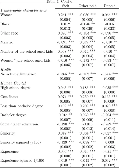
Demographics, health and human capital We again note that many coe¢ cients have di¤erent impact on paid and unpaid leave. This is the case for
1 2In the literature, the cost of absenteeism is usually related to an increased likelihood of
being …red or being passed up for promotion. Therefore, we settle on an indicator of the layo¤ rate (de…ned as the number of workers laid o¤ in the past year divided by average
the stock of human capital of the employee: higher levels of education, seniority or experience are associated with higher numbers of days of paid leave and lower numbers of days of unpaid leave. The magnitude of the increase in the number of paid sick leave diminishes however for higher levels of education. It is even negative for individuals with some higher education. Given the lack of information in the data, it is hard to conclude to a causal impact of education on absenteeism. It is possible that individual with some higher education are sorting into jobs where no sick leave is available. It should be noted though that good health, as an unambiguous impact, decreasing all types of absence.
The impacts of demographic characteristics are even more ambiguous, ex-plaining perhaps some contradictory results in the literature. For example, a women with no pre-school aged kids is more likely to take paid sick leave and unpaid leave but has less days of other paid leave. Adding pre-school aged kids increases both sick paid leave and other paid leave but decreases unpaid leave in the case of men and, surprisingly, decreases all three types of absence in the case of women. We interpret this as evidence that family responsabilities with respect to kids are more equally shared among parents than previously found.
Work arrangement and …rm size Three workplace characteristics un-ambiguously raise all types of absence: the compressed workweek, working in shift and being covered by a collective bargaining agreement. One could have thought that workers being covered by a collective bargaining agreement would have access to more paid leave thus lowering the need for unpaid leave but the results show that while an unionized worker is 15% and 20% more likely to get one day of paid sick or other paid leave, he is also more than twice as likely (52%) to take one day of unpaid leave. This seems to indicate a lower indirect cost of absenteeism.
more frequent in smaller workplace whereas other paid leave and especially sick paid leave is more likely to be observed in large workplaces.
Unobserved heterogeneity The estimated coe¢ cients for the unobserved heterogeneity distribution are shown in the last panel of Table 4. Remember that refers to unobserved workplace heterogeneity and to unobserved worker heterogeneity. At the worker level, since all are positive, this means that all types of absence are positively correlated: workers who take more paid sick leave also have more other paid leave and more unpaid leave. This indicates that there is probably a category of workers who are not very sensitive to the cost of absence.
However, at the workplace level, we observe a negative correlation between paid leave (sick or other) and unpaid leave. This means that workplaces with more paid sick leave also have more other paid leave but lower unpaid leave. Therefore, while summary statistics indicate that paid and unpaid leaves are substitutes, estimated correlations show that the substitutability is driven by the establishment leave policy and not by the worker.
6
Conclusion
This paper provides new evidence on the determinants of absence, distinguishing between three di¤erent types of absence and using that information to get some measure of the direct cost of absence to the worker. This paper is one of the very few articles examining the determinants of absences with survey data and a precise measure of the cost of absence.
We …nd that many workplace, worker or job characteristics have di¤eren-tiated impacts on paid and unpaid leave, something that has not been found
leisure is not an inferior good (positive income e¤ect and negative wage e¤ect). These e¤ects have opposite signs for paid leave which seems to indicate that the direct cost of absenteeism is lower for paid absences. Di¤erent e¤ects are also obtained for the layo¤ rate used as one proxy for the indirect cost of absen-teeism while the e¤ect is identical for the other proxy, the vacancy rate. Using an empirical model suitable to linked employer-employee data with workplace and worker unobserved heterogeneity, we …nd that all three types of absence are positively correlated at the worker level but that paid and unpaid leave are negatively correlated at the workplace level.
Further work would bene…t greatly to access to detailed contract informa-tion. For example, does the employee has access to any paid sick leave and if so how many days? Does the employee use unpaid leave only when paid leave is no longer available? Is the worker full compensated for sick leave or does he receive only a fraction of his wage?
References
Akyeampong, E. B. (2005). Fact sheet on work absences. Perspectives on Labour and Income 6 (4), 21–30.
Allen, S. G. (1981). An empirical model of work attendance. Review of Eco-nomics and Statistics 63 (1), 77–87.
Allen, S. G. (1983). How much does absenteeism cost. Journal of Human Resources 18 (3), 379–393.
Barmby, T. (2002). Worker absenteeism: a discrete hazard model with bivari-ate heterogeneity. Labour Economics 9, 469–476.
Barmby, T., C. Orme, and J. G. Treble (1991). Worker absenteeism: An analysis using microdata. Economic Journal 101 (405), 214–229.
Delgado, M. A. and T. J. Kiesner (1997). Count data models with variance of unknown form: An application to a hedonic model of worker absenteeism. Review of Economics and Statistics 79 (1), 41–49.
Dionne, G. and B. Dostie (2007). New evidence on the determinants of ab-senteeism using linked employer-employee data. Industrial and Labor Re-lations Review 61 (1), 106–118.
Dionne, G. and L. Eeckhoudt (1987). Proportional risk aversion, taxation and labour supply under uncertainty. Journal of Economics 47 (4), 353–366.
Drago, R. and M. Wooden (1992). The determinants of labor absence: Eco-nomic factors and workgroup norms across countries. Industrial and Labor Relations Review 45 (4), 764–778.
Dunn, L. and S. A. Youngblood (1986). Absenteeism as a mechanism for approaching an optimal labor market equilibrium: An empirical study. Review of Economics and Statistics 68 (4), 668–674.
Gollier, C. and L. Eeckhoudt (2000). The e¤ects of changes in risk and risk taking: A survey. In G. Dionne (Ed.), Handbook of Insurance, pp. 117–130. Kluwer Academic Press.
Gouriéroux, C., A. Monfort, and A. Trognon (1984). Pseudo maximum like-lihood functions: Applications to Poisson models. Econometrica 52 (3), 701–720.
Hausman, J., B. Hall, and Z. Griliches (1984). Econometric models for count data with an application to the patents-R&D relationship. Economet-rica 52, 909–938.
Heckman, J. and J. Walker (1990). The relationship between wages and in-come and the timing and spacing of births: Evidence from Swedish
longi-Henrekson, M. and M. Persson (2004). The e¤ects on sick leave of changes in the sickness insurance system. Journal of Labor Economics 22, 87–113.
Heywood, J. S. and U. Jirjahn (2004). Teams, teamwork and absence. Scan-dinavian Journal of Economics 106 (4), 765–782.
Ichino, A. and E. Moretti (2008). Biological gender di¤erences, absenteeism and the earning gap. American Economic Journal: Applied Economics.
Ichino, A. and R. T. Riphahn (2005). The e¤ect of employment protection on worker e¤ort: Absenteeism during and after probation. Journal of the European Economic Association 3 (1), 120–143.
Johansson, P. and M. Palme (2002). Assessing the e¤ect of public policy on worker absenteeism. Journal of Human Resources 37, 381–409.
Kauermann, G. and R. Ortlieb (2004). Temporal pattern in number of sta¤ on sick leave: the e¤ect of downsizing. Journal of the Royal Statistical Society Series C - Applied Statistics 53, 355–367.
Ose, S. O. (2005). Working conditions, compensation and absenteeism. Jour-nal of Health Economics 24, 161–188.
Vistnes, J. P. (1997). Gender di¤erences in days lost from work due to illness. Industrial and Labor Relations Review 50 (2), 304–323.
Wilson, N. and M. J. Peel (1991). The impact on absenteeism and quits of pro…t-sharing and other forms of employee participation. Industrial and Labor Relations Review 44 (3), 454–468.
7
Appendix: Comparative statics of
t
uand
t
p From (4) and (5) we obtain the following second order conditions:E ULL+ (w +weu)2UCC 2 (w +weu) UCL = Huu< 0 E ULL+ (w (1 s) +wep)2UCC 2 (w (1 s) +wep) UCL = Hpp< 0 E (ULL+ (w (1 s) +wep) (w +weu) UCC (weu+wep+ w (2 s)) UCL) = Hup= Hpu and Huu Hup Hpu Hpp = H > 0:
To obtain comparative statics results with respect to w, R, tc and E wi ,
we must …rst take the total di¤erentiation of the …rst order conditions:
Huudtu+ Hupdtp+ Huwdw + HuRdR + Hutcdtc+ HuE(wi) dE wi = 0 Hpudtu+ Hppdtp+ Hpwdw + HpRdR + Hptcdtc+ HpE(wi)dE wi = 0
from which we obtain the following results by applying the Cramer’s rule and writing i; j = p; u; j 6= i. @ti @R = Hjj H E ULC we itU CC where e wpt= w (1 s) +wep and e wut= w +weu:
This positive sign may become less important or even negative when s is high or close to one and for E (wp) E (wu) for a given U
LC.
In this model, tc is considered as exogenous when the worker makes his
decision about ti. So the e¤ect of @ti
@tc is given by the sign of:
Hjj
H E ULC we
itU
CC w:
Now di¤erentiating the …rst order conditions with respect to w yields for paid absence:
Huu
H E (1 s) UC+ ULC we
ptU
CC (tc (1 s) tp tu)
which is negative under normal conditions of positive labor supply curve and when s = 0. When s is su¢ ciently high or equal to one (full paid bene…ts), the e¤ect is positive when the income e¤ect is positive. The e¤ect becomes ambigu-ous for many values of s and is a subject matter for empirical investigation.
Finally, we may be interested to verify how an increase in the expected penalty may a¤ect the ti decisions. The sign of @ti
@E(wi) is the same as that of
@ti
@wi under certainty and is equal to:
Hjj
H E UC ULC we
itU CC ti
and is negative under the assumption that L is not an inferior good but becomes ambiguous otherwise. One can also rewrite the above equation and obtain:
Hjj H E 1 ULC weitUCC UC ti ! UC:
reduction in the optimal risk exposure following a …rst order deterioration in the random variable. It should be note, however, that a …rst-order deterioration in the random variable implies a decrease in its expected value while the contrary is not necessarily true (Gollier and Eeckhoudt (2000)).
T able 1: Su mmar y st atistics o n da y s of ab sen ce 1999-2004 All Sic k Ot h er paid Unp a id Da y s of a b se nce Mean Std D ev . Me a n Std D ev . Me a n Std D ev . Me an Std D ev . Sic k le a v e 1 .536 0. 016 4. 214 0. 005 2. 371 0. 044 1. 230 0. 024 Ot h er paid le a v e 0 .729 0. 010 1. 055 0. 019 4. 414 0. 052 0. 556 0. 019 Unp a id lea v e 1 .291 0. 016 0. 749 0. 006 0. 843 0. 023 6. 651 0. 010 #Obse rv ations 109,28 9 42,568 19,920 18,646
Table 2: Summary statistics - Employee
All Sick Other Unpaid Demographic characteristics
Women 0.518 0.589 0.535 0.546
Black 0.012 0.011 0.012 0.012
Other race 0.301 0.308 0.273 0.274 Married 0.559 0.584 0.61 0.471 Number of pre-school aged kids 0.238 0.255 0.238 0.23 Health
No activity limitation 0.611 0.586 0.581 0.603 Human Capital
High school degree 0.171 0.141 0.139 0.179 Certi…cate 0.137 0.119 0.14 0.159 Less than bachelor degree 0.397 0.434 0.412 0.409 Bachelor degree 0.13 0.171 0.159 0.09 Some higher education 0.059 0.075 0.079 0.03 Seniority 8.809 9.897 10.051 6.957 Experience 17.023 17.663 18.194 14.187 Income
Income from other sources (000s) 2.401 2.671 2.538 2.06 Wage Contract
Natural logarithm of hourly wage 2.841 2.973 2.981 2.664 Contracted hours 36.554 37.626 37.738 34.857 Work arrangement
Works regular hours 0.117 0.06 0.081 0.151 Usual workweek includes Sat. and Sun. 0.206 0.125 0.147 0.285 Work ‡exible hours 0.366 0.331 0.346 0.346 Does not work MtoF between 6am & 6pm 0.613 0.723 0.694 0.488 Some work done at home 0.245 0.294 0.304 0.13 Work some rotating shift 0.069 0.07 0.085 0.082 Work on a reduced workweek 0.068 0.043 0.052 0.105 Work on compressed work week schedule 0.053 0.047 0.058 0.063 Covered by a CBA 0.257 0.327 0.349 0.301
Table 3: Summary statistics - Workplace
All Sick Other Unpaid Cost of absenteeism E(wa)
Vacancy rate 0.018 0.018 0.018 0.019 Layo¤ rate 0.083 0.064 0.066 0.090 Size
20-99 employees 0.309 0.289 0.278 0.338 100-499 employees 0.204 0.246 0.255 0.207 500 employees and more 0.165 0.235 0.229 0.136 #Observations 109,289 42,568 19,920 18,646
Table 4: Simultaneous Poisson regressions on days of absence Sick Other paid Unpaid Variables from the theoretical model
Natural log. of hourly wage (w) 0.056 *** 0.148 *** -0.366 *** (0.004) (0.005) (0.005) Contracted hours (tc) 0.016 *** 0.021 *** -0.006 ***
(0.000) (0.000) (0.000) Income from -0.002 *** -0.001 *** 0.002 ***
other sources (000s) (R) (0.000) (0.000) (0.000) Cost of absenteeism ( E(wa))
Layo¤ Rate -0.012 *** -0.022 *** 0.004 ** (0.002) (0.002) (0.002) Vacancy Rate 0.075 *** 0.241 *** 0.219 ***
(0.024) (0.036) (0.028) Statistical signi…cance: *=10%; **=5%; ***=1%.
Table 4: Cont’d
Sick Other paid Unpaid Demographic characteristics Women 0.251 *** -0.030 *** 0.065 *** (0.004) (0.005) (0.006) Black 0.012 -0.046 ** -0.007 (0.013) (0.020) (0.023) Other race 0.028 *** -0.103 *** -0.096 *** (0.003) (0.005) (0.005) Married -0.091 *** 0.022 *** -0.010 ** (0.003) (0.004) (0.005) Number of pre-school aged kids 0.068 *** 0.014 *** -0.010 **
(0.003) (0.004) (0.004) Women * pre-school aged kids -0.016 *** -0.172 *** -0.093 ***
(0.005) (0.007) (0.007) Health
No activity limitation -0.365 *** -0.102 *** -0.265 *** (0.005) (0.007) (0.006) Human Capital
High school degree 0.043 *** 0.185 *** -0.035 *** (0.006) (0.008) (0.008) Certi…cate 0.074 *** 0.250 *** 0.136 ***
(0.005) (0.007) (0.009) Less than bachelor degree 0.102 *** 0.209 *** 0.023 ***
(0.005) (0.007) (0.008) Bachelor degree 0.015 ** 0.039 *** -0.204 ***
(0.007) (0.009) (0.011) Some higher education -0.190 *** -0.015 -0.289 ***
(0.008) (0.012) (0.014) Seniority 0.047 *** 0.034 *** -0.027 *** (0.001) (0.001) (0.001) Seniority squared (/100) -0.129 *** -0.098 *** 0.000 (0.002) (0.002) (0.003) Experience 0.006 *** 0.015 *** -0.031 *** (0.000) (0.001) (0.001) Experience squared (/100) -0.019 *** -0.045 *** 0.032 *** (0.001) (0.002) (0.002) Statistical signi…cance: *=10%; **=5%; ***=1%.
Table 4: Cont’d
Sick Other paid Unpaid Work arrangement
Work regular hours -0.337 *** -0.203 *** 0.197 *** (0.004) (0.005) (0.004) Work on weekend -0.110 *** -0.118 *** 0.011 **
(0.004) (0.005) (0.005) Work ‡exible hours -0.056 *** 0.018 *** 0.083 ***
(0.003) (0.003) (0.003) Work non traditional working hours 0.178 *** 0.154 *** -0.133 ***
(0.004) (0.005) (0.005) Work at home -0.025 *** 0.176 *** -0.227 ***
(0.003) (0.004) (0.005) Work in shift 0.220 *** 0.204 *** 0.011 * (0.005) (0.006) (0.007) Work on a reduced workweek -0.150 *** -0.162 *** 0.216 ***
(0.006) (0.007) (0.006) Work on compressed workweek 0.075 *** 0.136 *** 0.028 ***
(0.005) (0.006) (0.006) Covered by a CBA 0.151 *** 0.207 *** 0.520 *** (0.003) (0.005) (0.005) Firm Size 20-99 employees 0.324 *** 0.230 *** 0.137 *** (0.005) (0.006) (0.006) 100-499 employees 0.519 *** 0.351 *** 0.046 *** (0.006) (0.007) (0.007) 500 employees and more 0.647 *** 0.415 *** -0.074 ***
(0.007) (0.008) (0.009) Constant and unobserved heterogeneity parameters
Constant -2.169 *** -3.772 *** -0.638 *** (0.022) (0.026) (0.028) 0.556 *** 0.348 *** -0.842 *** (0.002) (0.003) (0.002) 0.688 *** 1.230 *** 1.749 *** (0.001) (0.002) (0.003) Industry dummies YES YES YES Occupation dummies YES YES YES
Year dummies YES YES YES
ln-likelihood -529,420.07
#observations 109,289
Statistical signi…cance: *=10%; **=5%; ***=1%. Robust standard error in parantheses