Collaborative concurrent mapping and localization

Collaborative Concurrent Mapping and

Localization

by

John William Fenwick

B.S. Physics, United States Air Force Academy, 1999

Submitted to the Department of Electrical Engineering and Computer

Science

in partial fulfillment of the requirements for the degree of

Master of Science in Electrical Engineering and Computer Science

at the

MASSACHUSETTS INSTITUTE OF TECHNOLOGY

June 2001

@

John William Fenwick, MMI. All rights reserved.

The author hereby grants to MIT permission to reproduce and

distribute publicly paper and electronic copies of this thesis document

in whole or in part.

A uthor ...

...

Department of Electrical Engineering and Computer Science

May1,,2001

C ertified by ...

...

... ...

...

Dr. Michael E eary

The Charles Stark Draper Laborat ry, Inc.

Technicil

Supervisor

Certified by...

Professor John J. Leonard

Associate Professor, DepprrpenfrQcean Engineering

Accepted by

Professor A. C. Smith

OF TACHN iffaE

OFATECHN ira a, Department Committee on Graduate Students

JUL 11

_ARCHIVES

LIBRARIES.-[This page intentionally left blank]

Collaborative Concurrent Mapping and Localization

by

John William Fenwick

Submitted to the Department of Electrical Engineering and Computer Science on May 21, 2001, in partial fulfillment of the

requirements for the degree of

Master of Science in Electrical Engineering and Computer Science

Abstract

Autonomous vehicles require the ability to build maps of an unknown environment while concurrently using these maps for navigation. Current algorithms for this con-current mapping and localization (CML) problem have been implemented for single vehicles, but do not account for extra positional information available when multi-ple vehicles operate simultaneously. Multimulti-ple vehicles have the potential to map an environment more quickly and robustly than a single vehicle. This thesis presents a collaborative CML algorithm that merges sensor and navigation information from multiple autonomous vehicles. The algorithm presented is based on stochastic estima-tion and uses a feature-based approach to extract landmarks from the environment. The theoretical framework for the collaborative CML algorithm is presented, and a convergence theorem central to the cooperative CML problem is proved for the first time. This theorem quantifies the performance gains of collaboration, allowing for determination of the number of cooperating vehicles required to accomplish a task. A simulated implementation of the collaborative CML algorithm demonstrates substantial performance improvement over non-cooperative CML.

Technical Supervisor: Dr. Michael E. Cleary

Title: Member of the Technical Staff, The Charles Stark Draper Laboratory, Inc. Thesis Advisor: Professor John J. Leonard

Title: Professor of Ocean Engineering

[This page intentionally left blank]

Acknowledgments

In spite of all my wishes, this thesis did not spontaneously write itself. I owe much thanks to those who helped and supported me through my time at MIT.

My parents, as always, provided steady support. Their gentle encouragement and pristine example provide all the direction I need for success in life.

Draper Laboratory provided the window of opportunity for higher education, and for this I will always be grateful. Dr. Michael Cleary provided much needed guidance to a novice engineer, giving me all the right advice at the right time. His patience with me was remarkable, especially considering that I always seemed to drop by at the most inopportune times. Mike's trust and confidence in my ability was the single most important element in making my MIT experience so rewarding.

Professor John Leonard is to be commended for his willingness to squeeze me into his already overloaded workload. He generously carved out a research niche for me and patiently let me follow it to completion. Many thanks also are extended to Dr. Paul Newman, who gave me innumerable tidbits of advice and guidance. Technical knowhow and lunch conversation dispensed by Rick Rikoski also helped keep me on the right track.

Thanks also to my roommates and all the other Air Force guys for helping me preserve my sanity. Red Sox games and beer were always a welcome study break. Finally, thanks to Nik, for putting everything in perspective and making my life so wonderful.

ACKNOWLEDGMENT (21 May 2001)

This thesis was prepared at the Charles Stark Draper Laboratory, Inc., under Internal Company Sponsored Research Project 13024, Embedded Collaborative Intelligent Systems.

Publication of this thesis does not constitute approval by Draper or the sponsoring agency of the findings or conclusions contained herein. It is published for

the exchange and stimulation of ideas.

Joipn W. Fenwick 21 May 2001

Contents

1 Introduction 17

1.1 Collaboration in mapping and localization . . . . 19

1.1.1 Motivating scenarios . . . . 19

1.1.2 Elements of CML . . . . 22

1.2 Single vehicle CML . . . . 24

1.2.1 Navigation techniques used in CML . . . . 24

1.2.2 _{Mapping techniques used in CML . . . .} 26

1.2.3 Feature-based CML . . . . 29

1.3 Collaborative CML . . . . 30

1.4 Summary . . . . 31

1.5 Contributions . . . . 32

1.6 Thesis organization . . . . 32

2 Single Vehicle Stochastic Mapping 33 2.1 _{Models . . . .} 33 2.1.1 Vehicle model . . . . 34 2.1.2 _{Feature model . . . . 35} 2.1.3 Measurement model . . . . 36 2.2 Stochastic mapping . . . . 38 2.2.1 SM prediction step . . . . 39 7

2.2.2 SM update step . . . . 41

2.3 Single vehicle CMVIL performance characteristics . . . . 44

2.4 Sum m ary . . . . 45

3 Extending CML to Multiple Vehicles 47 3.1 Critical challenges . . . . 47

3.2 Collaborative localization . . . . 48

3.2.1 Prediction step . . . . 49

3.2.2 Update Step . . . . 51

3.3 Collaborative CML . . . . 54

3.3.1 Collaborative CML prediction step . . . . 54

3.3.2 Collaborative CML update step . . . . 58

3.3.3 Collaborative CML performance analysis . . . . 62

3.4 Sum m ary . . . . 67

4 1-D Collaborative CML Simulation Results 69 4.1 1-D algorithm structure . . . . 70

4.1.1 Simulation parameters and assumptions . . . . 73

4.2 1-D R esults . . . . 74

4.2.1 1-D scenario #1 . . . . 74

4.2.2 1-D scenario #2 . . . . 78

4.2.3 1-D scenario #3 . . . . 81

4.3 Sum m ary . . . . 84

5 2-D Collaborative CML Simulation Results 85 5.1 Simulation assumptions . . . . 85

5.2 2-D Collaborative Localization Results . . . . 86

5.2.1 2-D CL scenario #1 . . . . 87

o.2.2 2-D CL scenario #2 . . . . 93 8

5.2.3 2-D CL scenario #3 . . . . 100 5.3 _{2-D Collaborative CML Results . . . 106} 5.3.1 2-D CCML scenario #1 . . . . 108 5.3.2 2-D CCML scenario #2 . . . . 116 5.3.3 2-D CCML scenario #3 . . . . 123 5.4 Sum m ary . . . 130

6 Conclusions and Future Research 131 6.1 _{Thesis contributions . . . 131}

6.2 Future research . . . 132

[This page intentionally left blank]

List of Figures

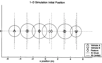
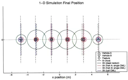
1-D scenario #1 initial position . . . . 1-D scenario #1 final position . . . .

1-D scenario #1 vehicle position versus time . . .

1-D scenario #1 vehicle A position error analysis

1-D scenario #1 vehicle B position error analysis

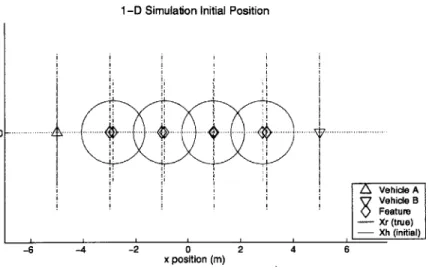
1-D scenario #2 initial position . . . ... . . . 1-D scenario #2 final position . . . .

1-D scenario #2 vehicle position versus time . . .

1-D scenario #2 vehicle A position error analysis 1-D scenario #2 vehicle B position error analysis

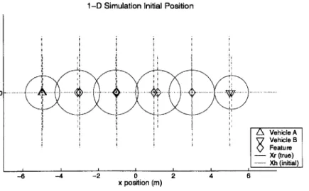
1-D scenario #3 initial position . . . . 1-D scenario #3 final position . . . .

1-D scenario #3 vehicle position versus time . . .

1-D scenario #3 vehicle A position error analysis 1-D scenario #3 vehicle B position error analysis

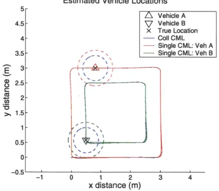
2-D CL scenario #1 : vehicle starting position . . . .

2-D CL scenario #1 : final position estimates . .

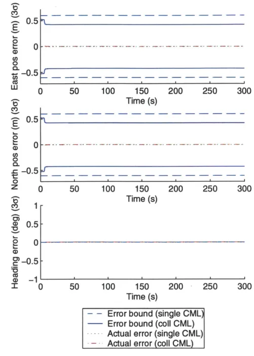
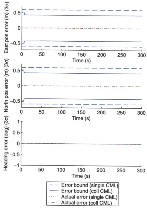
2-D CL scenario #1 position estimate comparison

2-D CL scenario #1 vehicle A error comparison

2-D CL scenario #1 vehicle B error comparison

11 4-1 4-2 4-3 4-4 4-5 4-6 4-7 4-8 4-9 4-10 4-11 4-12 4-13 4-14 4-15 5-1 5-2 5-3 5-4 5-5 . . . . 75 . . . . 76 . . . . 76 . . . . 77 . . . . 77 . . . . 78 . . . . 79 . . . . 79 . . . . 80 . . . . 80 . . . . 8 1 . . . . 82 . . . . 82 . . . . 83 . . . . 83 . . . . 88 . . . . 89 . . . . 89 . . . . 90 . . . . 9 1

5-6 5-7 5-8 5-9 5-10 5-11 5-12 5-13 5-14 5-15 5-16 5-17 5-18 5-19 5-20 5-21 2-D CL scenario #3 : 2-D 2-D 2-D 2-D 2-D 2-D 2-D 2-D 2-D 2-D 2-D 2-D CL scenario #1: 2-D CL scenario #1: 2-D CL scenario #2: 2-D CL scenario #2 2-D CL scenario #2: 2-D CL scenario #2 2-D CL scenario #2 2-D CL scenario #2 2-D CL scenario #2 2-D CL scenario #3 2-D CL scenario #3 2-D CL scenario #3 2-D CL scenario #3 2-D CL scenario #3 2-D CL scenario #3

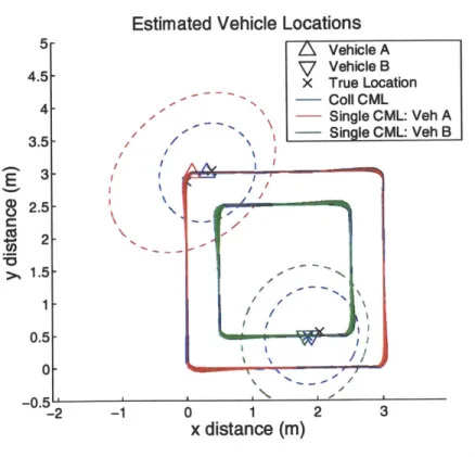
CCML scenario #1 : vehicle starting position .

CCML scenario #1 : final position estimates

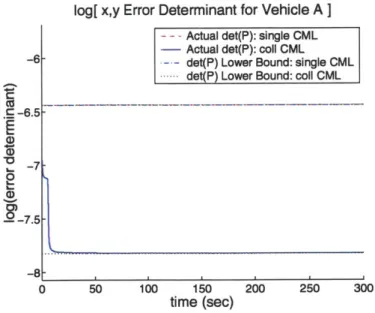
CCML scenario #1 : position estimate comparis CCML scenario #1 : vehicle A error comparison CCML scenario #1 : vehicle B error comparison CCML scenario #1 : vehicle A error determinan CL scenario #1 : vehicle B error determinant .

vehicle A error determinant vehicle B error determinant vehicle starting position . . .

: final position estimates .

position estimate comparison vehicle A error comparison vehicle B error comparison vehicle A error determinant vehicle B error determinant vehicle starting position . . . : final position estimates position estimate comparison vehicle A error comparison vehicle B error comparison vehicle A error determinant vehicle B error determinant

CCML scenario #1 : feature error determinant comparison

CCML scenario #2 : vehicle starting position . . . .

CCML scenario #2 : final position estimates . . . .

CCML scenario #2 : position estimate comparison . . . .

. . . 115 . . . 117 . . . 118 . . . 118 12 . . . . 92 . . . . 93 . . . . 94 . . . . 95 . . . . 96 . . . . 97 . . . . 98 . . . . 99 . . . . 100 . . . . 101 . . . . 102 . . . . 102 . . . . 103 . . . . 104 . . . . 105 . . . . 106 . . . . 110 . . . .111 on . . . .111 . . . . 112 . . . . 113 t . . . . 114 . . . . 114 5-22 5-23 5-24 5-25 5-26 5-27 5-28 5-29 5-30 5-31 5-32

5-33 5-34 5-35 5-36 5-37 5-38 5-39 5-40 5-41 5-42 5-43 5-44 comparison

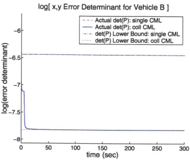
5-45 2-D CCML scenario #3 : feature error determinant comparison

13 2-D 2-D 2-D 2-D 2-D 2-D 2-D 2-D 2-D 2-D 2-D 2-D

CCML scenario #2: vehicle A error comparison CCML scenario #2 : vehicle B error comparison CCML scenario #2 : vehicle A error determinant CL scenario #2 : vehicle B error determinant . . .

CCML scenario #2 : feature error determinant CCML scenario #3 : vehicle starting position . . .

CCML scenario #3 : final position estimates .

CCML scenario #3 : position estimate comparison CCML scenario #3 : vehicle A error comparison CCML scenario #3 : vehicle B error comparison CCML scenario #3 : vehicle A error determinant CL scenario #3 : vehicle B error determinant . . .

. 119 . 120 . 121 . 121 . 122 . 124 . 125 . 125 . 126 . 127 . 128 128 129

[This page intentionally left blank]

CCML simulation global parameters ...

CCML simulation scenario #1 parameters . . . .

CCML simulation scenario #2 parameters . . . . CCML simulation scenario #3 parameters . . . .

Collaborative Localization simulation global parameters

CL simulation scenario #1 parameters . . . . CL simulation scenario #2 parameters . . . . CL simulation scenario #3 parameters . . . . Collaborative CML simulation global parameters . . . . CCML simulation scenario #1 parameters . . . . CCNL simulation scenario #2 parameters . . . . CCNMJL simulation scenario #3 parameters . . . .

15

List of Tables

[This page intentionally left blank]

Chapter 1

Introduction

Successful operation of an autonomous vehicle requires the ability to navigate. Nav-igation information consists of positional estimates and an understanding of the sur-rounding environment. Without this information, even the simplest of autonomous tasks are impossible. An important subfield within mobile robotics that requires accurate navigation is the performance of collaborative tasks by multiple vehicles. Multiple vehicles can frequently perform tasks more quickly and robustly than a sin-gle vehicle. However, cooperation between vehicles demands the vehicle be aware of relative locations of collaborators in addition to the baseline environmental knowl-edge.

Current solutions to autonomous vehicle localization rely on both internal and ex-ternal navigational aides. Inex-ternal navigation instruments such as gyros and odome-ters (on land vehicles) provide positional estimates, but are susceptible to drift and thus result in a navigation error that grows linearly with time. This unbounded error growth makes long-term autonomous operation using only internal devices im-possible. Beacon systems (such as the Global Positioning System (GPS) ) provide extremely accurate navigation updates, but require pre-placement of accessible bea-cons (satellites). In the case of GPS, this limits use to outdoor open-air environments.

Autonomous Underwater Vehicles (AUVs), as well as autonomous land vehicles op-erating indoors, are unable to utilize GPS as a result. Acoustic beacon arrays with known locations have been used successfully by AUVs for navigation, but deployment of such beacons is only feasible in a limited number of mission scenarios. AUVs have demonstrated the ability to localize their position and navigate using accurate a priori bathymetric maps, but a priori knowledge of the underwater environment is not al-ways available, especially in littoral zones where the environment frequently changes in ways that would affect a shallow water AUV. A recent advance in autonomous vehicle navigation techniques, Concurrent Mapping and Localization (CML), incor-porates environmental data to provide vehicle position information [46]. CML allows an autonomous vehicle to build a map of an unknown environment while simulta-neously using this map to improve its own navigation estimate. This technique has been demonstrated both in simulation and on actual vehicles.

This thesis reports the execution of the logical next step in the development of CML: a CML algorithm for use by multiple collaborating autonomous vehicles. Sharing and combining observations of environmental features as well as of the col-laborating vehicles greatly enhances the potential performance of CML. This thesis is demonstrates the feasibility and benefits of collaborative CML. Multiple vehicles performing CML together perform faster and more thorough mapping, and produce improved relative (and global) position estimates. This thesis quantifies the improve-ment in CML performance achieved by collaboration, and compares collaborative versus single-vehicle CML results in simulation to demonstrate how collaborative CML greatly increases the navigation capabilities of autonomous vehicles.

This chapter reviews the fields within mobile robotics that are most relevant to this thesis. Section 1.1 discusses the importance of collaboration, then briefly surveys current collaborative techniques in mapping and navigation. In Section 1.2, the field of single-vehicle CML is described. The intersection of these two fields is collaborative

INTRODUCTION

1.1 COLLABORATION IN MAPPING AND LOCALIZATION

CML, discussed in Section 1.3, which provides motivation for the work of this thesis and also reviews current collaborative CML implementations. The contribution made by this thesis is described in Section 1.5. The chapter closes with a presentation of the organization of the thesis in Section 1.6.

1.1

Collaboration in mapping and localization

A team of collaborating autonomous vehicles can perform certain tasks more effi-ciently and robustly than a single vehicle [1, 383, and thus have been the focus of significant study by the robotics community in the past decade. Section 1.1.1 moti-vates the need for teams of autonomous vehicles to localize themselves with respect to their surroundings and each other, as well as collaborative construct maps of their en-vironments. Current work in collaborative localization is reviewed in Section 1.1.2.1, and a brief survey of collaborative mapping is presented in Section 1.1.2.2. More detailed reviews of collaboration in mobile robots are presented in Cao et al. [10], Parker [38], and Dudek et al. [18].

1.1.1

Motivating scenarios

The following discussion of possible applications for teams of autonomous vehicles that are able to perform localization and mapping demonstrates why collaborative CML is of interest.

1.1.1.1 Indoor search and rescue

Autonomous vehicles perform tasks without endangering the life of their operator, making them attractive for firefighting or search and rescue. Often firefighters or rescue personnel put themselves at great risks to search for victims inside buildings. A team of autonomous vehicles that could perform these tasks quickly and effectively 19

INTRODUCTION

would be helped by being able to collaboratively map the building while searching for victims. Furthermore, a heterogenous combination of vehicles could include very small, speedy search vehicles, as well as bigger firefighting or rescue vehicles to be summoned when needed. Accurate navigation and mapping is essential to to perform this task, and a team of robots able to collaboratively localize and map the search area would provide the robustness and search efficiency needed for successful search and rescue.

1.1.1.2 Submarine surveillance

The military seeks the capability to covertly observe the departure of an adversary's submarines from their home ports. Detection of submarines in the open ocean is much harder than detection in shallow water at a known departure point. One cur-rent option available to the Navy is to position static acoustic listening devices on the the sea floor or on the surface. However, these are difficult to deploy, requiring divers or aircraft for delivery. Submarines themselves can also perform surveillance, but they are limited to deep water operations. The inability of such submarines to operate in shallow water and the limited range of underwater sensors gives an adver-sary a window of opportunity to escape detection. Surveillance would be performed much more effectively by an array of shallow water AUVs. By staying within com-munications range and cooperatively localizing with respect to each other, a web of properly positioned AUVs could create a barrier through which an adversary could not slip through undetected. This AUV array could be deployed quickly, easily, and covertly. This mission emphasizes the need for AUVs to share map and navigation information in order to maintain proper relative positioning as well as to detect the enemy submarine.

1.1 COLLABORATION IN MAPPING AND LOCALIZATION

1.1.1.3 _{Close proximity airborne surveillance}

A major advantage of autonomous air vehicles over conventional aircraft is the

in-creased maneuverability envelope gained by eliminating the pilot, as their smaller size is coupled with a much higher tolerance for tight turns (which induce high 'G' forces). Capitalizing on this maneuverability while in close proximity to obstacles (such as the ground, foliage, or other aircraft) requires excellent navigation and mapping ca-pabilities. One military mission that requires extremely low altitude, high-precision navigation and mapping is close-proximity surveillance of an unknown enemy posi-tion. Military operations benefit greatly from real-time observations, especially in the minutes leading up to an attack. Multiple autonomous air vehicles could gather this coveted information by entering into and observing an enemy position when the potential gain is worth the loss of surprise. Collision avoidance is especially crucial in this situation, since survivability demands that these vehicles be able to hide behind buildings, trees, and other terrain features. Further, relative position information is essential to avoid collisions with collaborators. Using multiple vehicles for this task increases the likelihood of mission success and decreases the amount of time required to complete the surveillance.

1.1.1.4 Summary

Enabling autonomous vehicles to share navigation and map information would greatly extend the existing performance capabilities of autonomous vehicles in a variety of vehicle domains. These existing capabilities are demonstrated by the current work in the fields of collaborative navigation and collaborative mapping, presented in the

next section.

1.1.2

Elements of CML

CML is the combination of mapping and localization. Existing work on these two tasks as separate tasks is presented next.

1.1.2.1 Collaboration in navigation

Collaborative navigation is performed when multiple vehicles share navigation and sensor information in order to improve their own position estimate beyond what is possible with a single vehicle. This section surveys existing work in improving navi-gation through collaboration.

Ant-inspired trail-laying behaviors have been used by a team of mobile robots tasked to navigate towards a common goal [55]. In this implementation a robot communicates its path to collaborators upon successfully arriving at the goal via a random walk. Sharing this information improves the navigational ability of all the robots.

Simple collective navigation has been demonstrated in simulation using multiple 'cartographer' robots that randomly explore the environment [13]. These vehicles possess no pose estimate, and are only capable of line-of-sight communication. When one of these robots detects the goal, it transmits this fact to all other robots it cur-rently observes, and then passes the data along in the same manner. A 'navigator' robot then uses this propagated communication signal to travel to the goal by using the cartographer robots as waypoints.

Simple relative localization between collaborators has been performed using direc-tional beacons [50]. Vision-based cooperative localization has been performed by a team of vehicles tasked with cooperatively trapping and moving objects [49]. Track-ing via vision is also used for relative localization of collaborators in an autonomous mobile cleaning system [26].

In work by Roumeliotis et al. [41,42], collaborative localization is performed

us-IN TRODUCT ION

1.1 COLLABORATION IN MAPPING AND LOCALIZATION

ing a distributed stochastic estimation algorithm. Each vehicle maintains its own navigation estimate, and communicates localization information only when directly observing a collaborator.

Cooperative navigation of AUVs has been performed in work by Singh et al. [45]. Also, two AUVs have demonstrated collaborative operation using the same acoustic beacon array [2]. An unmanned helicopter has used a vision sensor to detect collabo-rating ground vehicles at globally known positions, and thus was able to localize itself [56].

A related field to collaborative localization is use of multiple vehicles to construct maps of the environment, and is explored in the next section.

1.1.2.2 Collaboration in mapping

Collaborative mapping is performed by combining sensor information from multiple vehicles to construct a larger, more accurate map. Cooperative exploration and map-ping with multiple robots is reported by Mataric [32] using behavior-based control [9]. Map matching is used to combine topological maps constructed by multiple vehicles in work performed by Dedeoglu and Sukhatme [15] (Topological maps are described in Section 1.2.2.3).

Heterogenous collaborative mapping has also been investigated, as such systems can capitalize on specialization. One example is a mapping implementation comprised of 'worker' robots which constantly search the environment, and a static 'database' robot that communicates with and is visited by the worker robots [7]. The database robot maintains a centralized, global representation of the environment.

1.2

Single vehicle CML

Most collaborative navigation and mapping techniques have a single-vehicle naviga-tion and mapping technique as the basis, since collaborating vehicles must be able to operate independently in the event of loss of communication. Robust, collision-free operation of an autonomous vehicle requires a description of the vehicular pose as well as information about the location of objects in the vehicle's environment. Only with knowledge of self and surroundings can a safe path of travel can be calculated.

Section 1.2.1 describes common navigation techniques underlying CML. Similarly, Section 1.2.2 reviews the main techniques used for autonomous vehicle mapping. The intersection of these two related fields is Concurrent Mapping and Localization (CML), in which an autonomous vehicle builds a map of an unknown environment while simultaneously using this map to improve its own navigation estimate. Existing CML work can be partitioned by the mapping approaches presented in Section 1.2.2. Feature-based CML, the subset of CML most applicable to work in this thesis, is reviewed in greater detail in Section 1.2.3.

1.2.1

Navigation techniques used in CML

Understanding the need to improve improve techniques for autonomous vehicle nav-igation requires an understanding of the shortcoming of current approaches to the navigation problem. A detailed survey of localization techniques can be found in Borenstein, Everett, and Feng [8]. This subsection reviews the primary methods used; dead-reckoning and inertial navigation, beacon-based navigation, and map-based navigation.

IN TRODUCT ION

1.2 SINGLE VEHICLE CML

1.2.1.1 Dead reckoning and inertial navigation systems

Dead reckoning is accomplished by integrating velocity or acceleration measurements taken by the vehicle in order to determine the new vehicle position. This task is most often performed by inertial navigation systems (INS), which operate by integrating the acceleration of the vehicle twice in time to compute a new position estimate. These systems use accelerometers and gyroscopes to sense linear and angular rate. INS suffers from accuracy problems resulting from integration errors. Another inter-nal data source for state determination on land robots is odometry, which measures wheel rotation. This estimate is affected by wheel slippage, which can be significant in a number of situations [8].

Dead reckoning is the most commonly used AUV navigation technique. Unfor-tunately, the vehicle is only able to measure its velocity with respect to the water column, not accounting for drift caused by ocean currents. This can be an especially significant safety hazard for AUVs that operate at low speeds and in shallow water, due to the proximity of the ocean floor. Historically, INS use in AUVs has also been made difficult by power consumption and cost. The basic problem with reliance on either dead reckoning or INS devices is the same - position error grows without bound as the vehicle travels through the environment.

1.2.1.2 Beacon-based navigation

The placement of artificial beacons at known locations allow autonomous vehicles to determine their position via triangulation. The most prevalent beacon-based naviga-tion system is the satellite-based Global Posinaviga-tioning System (GPS), which provides worldwide localization with an accuracy of meters. GPS is an excellent navigation solution for a great number of mobile robot implementations, but is not applicable in all cases. Specifically, GPS signals are not strong enough to be used indoors and underwater, and in military applications GPS use can be denied by signal jamming.

Beacon-based navigation by AUVs uses an array of acoustic transponders placed in the environment. Sound pulses emanating from these beacons and prior knowledge about the transponder locations are combined to calculate the AUV position. The two primary beacon systems currently used are ultra-short baseline (USBL) and long baseline (LBL). Both systems rely on accurate beacon deployment and positioning. While beacon-based navigation is the system of choice for AUV applications, bea-con deployment during covert military operations in other difficult areas (as under the polar ice cap) can be significant handicaps. Currently GPS is crucial for truly autonomous operation of unmanned air vehicles, as even the slightest of positional errors can have disasterous consequences, especially during takeoff and landing.

1.2.1.3 Map-based navigation

Often it is infeasible to provide artificial beacons for navigation. Instead, map-based navigation techniques use the natural environment and an a priori map for localiza-tion. By comparing sensor measurements with the ground truth map, current vehicle pose can be deduced. Thompson et al. [52] performed localization by matching vis-ible hills and other naturally occuring terrain features on the horizon to an a priori topological map. Cozman and Krotkov [13] also visually detect mountain peaks on the horizon, then localize probabilistically using a known map. Cruise missiles have successfully used terrain contour matching (TERCOM) via a radar altimeter and an a priori map to localize their position [23].

1.2.2

Mapping techniques used in CML

Generally, autonomous vehicle mapping approaches can be grouped by how the map is constructed and environmental information is stored. The basic techniques of map construction elicit entirely different solution spaces, and by this criteria map-ping approaches can be grouped into grid-based, feature-based, and topological-based

IN TRODUCT ION

1.2 SINGLE VEHICLE CML

approaches.

1.2.2.1 Grid-based map representation

Grid-based approaches, such as those described by Moravec [34], represent the envi-ronment via an evenly-spaced grid. Each grid cell contains information about possible obstacles at that location. In most cases a probability between 0 and 1 is stored in each cell. A probability of 1 is assigned if the cell is certain to be occupied, and a probability of 0 if it is certain to be free. A map constructed in this fashion is called an occupancy or certainty grid. Mapping is performed by incorporating new mea-surements of the environment into the occupancy grid, and these meamea-surements are incorporated by increasing or decreasing the probability values in the corresponding grid cells. Localization is performed by a technique called map matching. A local map consisting of recent measurements is generated and then compared to a previously constructed global map. The best map match is found typically by correlating the local to the global map, and from this match the new position estimate is generated. Based on this position, the local map is then merged into the global map.

Work by Thrun et al. [53] represents the current state of the art of implementa-tions of the grid-based map representation. This method has also been implemented by Yamauchi et al. [57] and Salido-Tercero et al. [44]. Grid based map representa-tions are simple to construct and maintain, and directly incorporate all measurement data into the map. However, grid-based approaches suffer from large space and time complexity. This is because the resolution of a grid must be great enough to capture every important detail of the world. Performance is also highly dependent on the quality and model of sensors used for the map update. Also, information is lost when measurements are assigned to grid cells.

1.2.2.2 Feature-based map representation

Feature-based approaches to mapping represent environments using a set of geomet-ric attributes such as points, planes, and corners, and encode these landmarks in a metrically accurate map [31]. This representation has its roots in surveillance and target tracking [4].

1.2.2.3 Topological-based map representation

Topological-based approaches to mapping produce graph-like descriptions of environ-ments [16]. Nodes in the graph represent 'significant places' or landmarks [28]. Work by Chatila and Laumond [12] exemplifies this approach. Once created, the topologi-cal model can be used for route planning or similar problem solving purposes. Arcs connecting the nodes depict the set of actions required to move between these sig-nificant places. For instance, in a simple indoor environment consisting entirely of interconnected rooms, the topological map can represent each room as a node and the actions needed to travel between rooms as arcs. Computer vision has been used to characterize places by appearance, making localization a problem of matching known places with the current sensor image [51]. The topological approach can produce very compact maps. This compactness enables quick and efficient symbolic path planning, which is easily performed by traversing the graph representation of the environment. The major drawback to the topological approach is difficulty in robustly recognizing significant places. Regardless of the sensor used, identification of significant places, especially in a complex environment (e.g. an outdoor environment), is very sensitive to point of view [27, 28]. Further, distinguishing between similar-looking significant places is difficult, in part because no metric map is maintained.

INT RODUCT ION

1.2 SINGLE VEHICLE CML

1.2.2.4 Summary

The three mapping approaches have many orthogonal strengths and weaknesses. All the approaches, however, exhibit increased computational complexity when the size of the environment to be mapped is increased. Another common difficulty with these approaches is the need to robustly handle ambiguities in the sensor measurements.

The problem of data association is compounded in the feature and topological-based approach, which use frequently unreliable sensor measurements for accurate identifi-cation of features within the environment.

1.2.3

Feature-based CML

A significant challenge for mobile robotics is navigation in unknown environments when neither the map nor vehicle position are initially known. This challenge is ad-dressed by the techniques for Concurrent Mapping and Localization (CML). CML approaches can be categorized by the map representations described in Section 1.2.2. This section focuses on the subset of the field, feature-based CML, which is the rep-resentation of choice for work presented in this thesis. Work in grid-based CML

[3, 20, 21, 54, 57] is less relevant in this context.

Feature-based approaches to CML identify stationary landmarks in the environ-ment, then use subsequent observations of these landmarks to improve the vehicle navigation estimate. An example of this approach is work by Deans and Hebert [14], which uses an omnidirectional camera and odometry to perform landmark-based CML.

Stochastic Mapping (SM) [47] (discussed in further detail in Chapter 2) provides the theoretical foundation for the majority of feature-based CML implementations. In Stochastic Mapping, a single state vector represents estimates of the vehicle loca-tion and of all the features in the map. An associated covariance matrix incorporates the uncertainties of these estimates, as well as the correlations between the estimates. 29

The heart of Stochastic Mapping is an Extended Kalman Filter (EKF) [5,22], which uses sensor measurements and a vehicle dead reckoning model to update vehicle and feature estimates. Stochastic Mapping capitalizes on reobservation of static features to concurrently localize the vehicle and improve feature estimates. Analysis of theo-retical Stochastic Mapping performance is presented by Dissanayake et al. [17] and in further detail by Newman [37].

Adding new features to the state vector produces a corresponding quadratic ex-pansion to the system covariance matrix, and computational complexity thus becomes problematic in large environments. Feder [19] addresses the complexity issue by main-tains multiple local submaps in lieu of a single, more complex global map.

Another challenge inherent in Stochastic Mapping is feature association, the pro-cess of correctly matching sensor measurements to features. Feature association tech-niques have been successfully demonstrated in uncluttered indoor environments [6], but remain a challenge for more geometrically complex outdoor environments.

The Stochastic Mapping approach to feature-based CML serves as the algorithmic foundation for this thesis. Current implementations of the collaborative extensions to CML are discussed in the next section.

1.3

Collaborative CML

This section reviews related work most similar to that presented in this thesis, the in-tersection of the fields of autonomous vehicle collaboration and CML. One navigation method for collaborative navigation and mapping uses robots as mobile landmarks for their collaborators. Kuipers and Byun [29, 30] introduce this concept, whereby some robots move while their collaborators temporarily remain stationary. This method is extended through the use of synchronized ultrasound pulses to measure the distances between team members and determination the relative position of the vehicles via

triangulation [36]. This system has been implemented on very small (5 cm) robots [24]. Another such implementation uses an exploration strategy that capitalizes on line of sight visual observance between collaborators to determine free space in the environment and reduce odometry error [40]. Drawbacks to this approach are that only half of the robots can be in motion at any given time and the robots must stay close to each other in order to remain within visual range.

An important challenge in collaborative robotics is the task of combining maps that were independently gathered by cooperating vehicles. The first step in accom-plishing this task is vehicle rendezvous, the process of determining the relative location of each vehicle with respect to its collaborators. This is not trivial when vehicles have previously been out of sensor range, out of communication, or have a poor sense of global position. Rendezvous has proved workable in an unknown environment given unknown starting positions using landmark-based map matching [43]. Rendezvous has been detected visually, following which the shared maps are combined probabilis-tically [20]. Map merging has also been demonstrated once rendezvous is complete [25,39].

1.4

Summary

This chapter introduced and motivated the underlying techniques for collaborative concurrent mapping and localization. Possible applications requiring improved navi-gation and mapping performance for multiple vehicles were presented. Current work in autonomous vehicle collaboration, navigation, and mapping was reviewed to place the work performed in this thesis into the correct context, with focus given to the the subset of CML that this thesis extends - the Stochastic Mapping approach to feature-based CML.

1.5

Contributions

This thesis makes the following contributions:

e A method for performing collaborative concurrent mapping and localization.

o A quantitative theoretical analysis of the performance gains of that collabora-tion method.

o An analysis of collaborative concurrent mapping and localization performance in 1-D and 2-D simulation.

1.6

Thesis organization

This thesis presents an algorithm for performing CML with multiple vehicles working cooperatively. The remainder of it is structured as follows.

Chapter 2 reviews stochastic mapping as a theoretical foundation for performing single-vehicle CML.

Chapter 3 extends the stochastic mapping algorithm to multiple vehicles. An algorithm for collaborative dead-reckoning in the absence of static environmental fea-tures is discussed. A collaborative CML algorithm is then introduced and developed. Theoretical analysis of this algorithm generates a convergence theorem that quantifies the performance gain from collaboration.

Chapter 4 applies the collaborative CML algorithm in a 1-D simulation, to explain the algorithm structure and demonstrate its performance.

Chapter 5 presents 2-D simulations of both collaborative localization and collab-orative CML with varying parameters.

Chapter 6 summarizes the main contributions of this thesis and provides sugges-tions for future research.

Chapter 2

Single Vehicle Stochastic Mapping

Most successful implementations of feature-based CML use an Extended Kalman Filter (EKF) [5, 22] for state estimation. The class of EKF-based methods for feature-based CML is termed stochastic mapping (SM) [35, 47].

This chapter reviews the single vehicle stochastic mapping algorithm which will be extended to incorporate collaboration in Chapter 3. Section 2.1 presents the representations used in the stochastic mapping process, followed by a brief overview in Section 2.2 of the stochastic mapping algorithm itself. For a more detailed explanation refer to one of Smith, Self, and Cheeseman's seminal papers on SM [47,48].

2.1

Models

This section presents the form of the vehicle, observation, and feature models to be used in this thesis. To preserve simplicity for presentation purposes, these models are restricted to two dimensions.

2.1.1

Vehicle model

The state estimate for an autonomous vehicle in this implementation is represented by

xV = [XV Yv

#

well as heading and speed. Vehicle movement uv[k] due to control input is generated at time k with time T between successive updates, and consists of a change in heading and a change in speed, such that

uV[k] = 0 0 T6$[k] T6v[k] (2.1)

and is assumed to be known can be defined as

exactly. The general form of a vehicle dynamic model

x [k + 1] = f(xv[k], uv[k]) + wv[k] . _(2.2)

This discrete time vehicle model describes the transition of the vehicle state vector x, from time k to time k + 1 and mathematically takes into account the kinematics and dynamics of the vehicle. The function f is a nonlinear model that receives the current vehicle state xv[k] and control input u,[k] as inputs. The model is updated at times t = kT for a constant period T, and can be expanded and written as

f(xv[k], uv[k]) =

x[k] + Tcos(q[k])v[k] y[k] + Tsin(#[k])v[k]

0[k] + T6q[k] v[k] + Tov[k]

Although this particular vehicle dynamic model is non-linear, it can be linearized using its Jacobian evaluated at time k [33]. The Jacobian is linearized based on the (2.3)

2.1 MODELS

vehicle state, such that

x,[k + 1] = Fv[k]xv[k] + uv[k] +w, . (2.4)

The dynamic model matrix F,[k] is the Jacobian of f with respect to the vehicle state, and is defined as

- Tsin($[k])v[k] Tcos(o[k])v[k] 1 0 Tcos(4[k]) Tsin(O[k]) 0 1

Noise and the unmodeled components of the vehicle behavior are consolidated into the random vector w,. This vehicle model process noise is assumed to be a stationary, temporally uncorrelated zero mean Gaussian white noise process with covariance

E[4, wL4 = xwV 0 0 0 0 Yw) 0 0 0 0 okw 0 0 0 0 vw (2.6)

2.1.2

Feature model

Features are fixed, discrete, and identifiable landmarks in the environment. Repeat-able observation of features is a core requirement for CML. These features can take many forms, including passive features (points, planes, and corners), or active fea-tures (artificial beacons). What constitutes a feature is entirely dependent on the physics of the sensor used to identify it. Vision systems, for instance, may be able to identify features based on color, whereas sonar and laser rangefinders use distance and reflectivity to categorize features.

F v [k] -1 0 0 0 0 1 0 0 (2.5) 35

This thesis uses, without loss of generality, the least complicated of features, sta-tionary point landmarks. This simplification reduces challenges with feature identifi-cation and interpretation, increasing the focus on the CML algorithm itself. A point feature is defined by two parameters specifying its position with respect to a global reference frame, and is observable from any angle and any distance. The feature state estimate parameters of the itl point landmark in the environment are represented by

Xf = .: _(2.7)

Yfi

The point feature is assumed to be stationary, so unlike the vehicle model, there is no additive uncertainty term due to movement in the feature model. Therefore the model for a point feature can be represented by

Xfi[k +

Ilk]

2.1.3

Measurement model

A measurement model is used to describe relative measurements of the environment taken with on-board sensors. In this thesis range measurements are provided by sonar, which operates by generating a directed sound pulse and timing the reflected return off features in the environment. With knowledge of the speed of sound and the pulse duration, the distance to the reflecting surface is deduced. Inexpensive sonars are easily installed on mobile robots but present some significant challenges due to often ambiguous and noisy measurements. Sonar pulses have a finite beam width, producing an angular uncertainty as to the direction of the reflecting surface. Drop-outs, another problem, occur when the physical structure of the reflecting surface is too poor to generate a reflection capable of being detected. A multipath return occurs when a sonar pulse reflects off multiple surfaces before being detected, thus producing

an overly long time of flight. Lastly, when using an array of multiple sonars, crosstalk is possible. This occurs when a sonar pulse emanating from one sonar transducer is detected by another, producing an erroneous time of flight. These attributes of sonar are taken into account by incorporating noise into the sonar model.

The measurement model is used to process sonar data readings in order to deter-mine where features are in the environment. An actual sonar return

V_ [ k]

zi[k] =

i

consisting of a relative range vz,[k] and bearing z, [k] measurement is taken at time k from the vehicle with state xv[k] to the ith feature with state xfj[k]. The model for the production of this reading is given by

zi[k] = hi(xv[k], xf,[k]) + wi[k] , (2.10) where hi is the observation model which describes the nonlinear coordinate trans-formation from the global to robot-relative reference frame. Noise and unmodeled sensor characteristics are consolidated into an observation error vector wi[k]. This vector is a temporally uncorrelated, zero mean random process such that

Rz = E[wi[k] wi[k]'] = rw 0 , (2.11)

0 We

where R, _{is the observation error covariance matrix. The measurement function can}

be expanded and written as

[k])

h~xVk]x~[])= arctan ( fb.[k] y,[] -

O[k]

1

x Xf[ [k]xk - X[k][) =

Improving navigation performance in stochastic mapping relies on comparing pre-dicted and actual measurements of features. Prepre-dicted measurements are calculated based on the current location of the vehicle and environmental features as well as the observation model. Therefore a predicted sonar return taken at time k from the vehicle with state x,[k] to the i h feature with state xf, [k] has the form

ii[k] = hi(x,[k], xf,[k]) . (2.13)

2.2

Stochastic mapping

Stochastic mapping (SM), first introduced by Smith, Self and Cheeseman [48], pro-vides a theoretical foundation of feature-based CML. The SM approach assumes that distinctive features in the environment can be reliably extracted from sensor data. Stochastic mapping considers CML as a variable-dimension state estimation problem, where the state size increases or decreases as features are added to or removed from the map. A single state vector is used to represent estimates of the vehicle location as well as all environmental features. An associated covariance matrix contains the uncertainties of these estimates, as well as all correlations between the vehicle and fea-ture estimates. SM capitalizes on reobservation of stationary feafea-tures to concurrently localize the vehicle and improve feature estimates. The implementation of stochastic mapping applied by this thesis uses the vehicle, feature, and sonar measurement mod-els detailed in Sections 2.2.1, 2.2.2, and 2.2.3, respectively. Assuming two stationary features, this section presents the EKF-based algorithms that constitute SM.

SINGLE VEHICLE STOCHASTIC MAPPING 38

2.2.1

SM prediction step

Stochastic mapping algorithms used for CML use a single state vector that contains both the vehicle and feature estimates, denoted by

A predicted estimate given the motion commands provided to the vehicle is generated using the vehicle model described in Equations 2.4 and 2.5, producing a predicted

x[k + Ilk] with the form

xv[k + Ilk] xf[k+l|k] =F[k]x[k]+u[k]+w[k] Xf2[k+l|k]

j

Fv[k]xv[k]

1

The feature state estimates in the prediction stage are unchanged, as the features themselves are assumed to be stationary. Unlike the features, the vehicle is in motion,

x[k + Ilk]

and because of the uncertainty in this motion the system noise covariance model

QV

Q

=

0 0 0

adds noise to the vehicle estimate. Associated with the state estimate x[k] is an estimated covariance matrix P[k], which has the general form

P[k + Ilk] = F[k]P[klk]FT [k] +Q . (2.17)

In its expanded form, the estimated covariance matrix

Pvv[k] Pv1[k] Pv2[k]

P[k] = P1v[k] Pv1[k] PN[k] (2.18)

P24[k] P2 1[k] P2 2[k]

contains the vehicle (Pv[k]) and feature (Pii[k]) covariances located on the main diagonal. Also contained are the vehicle-feature (Pri[k]) and feature-feature (Pij[k]) cross correlations, located on the off-diagonals. Maintaining estimates of cross cor-relations is essential for two reasons. First, information gained about one feature can be used to improve the estimate of other correlated features. Second, the cross correlation terms prevent the stochastic mapping algorithm from becoming overconfi-dent, the result incorrectly assuming features are independent when they are actually correlated [11].

At each time step a prediction is made by Equation 2.4 even if no sensor measure-ments are taken. The prediction step, used on its own, enables the vehicle to perform dead-reckoning.

SINGLE VEHICLE STOCHASTIC MAPPING

2.2.2

SM update step

The update step in stochastic mapping integrates measurements made of features in the environment in order to create a map of the environment as well as improve the vehicle's own state estimate. Sensor ranging observations measure the relative dis-tance and orientation between the vehicle and features in the environment. Applying Equation 2.10, a predicted measurement from the vehicle to feature 1 is

21[k + 1] = _{h(xv[k +} lIk], x,[k]) = V21[ki

]

- 2,[k+1]

Thus a full predicted measurement set of all features in the environment is defined as

2[k + 1|k] = 21[k + 1k]

i2[k + Ilk]

h(x[k + 1|k], xf,[k]) _(2.20) h(x,[k + Ijk], xf. [k])

An algorithm is then used to associate the predicted measurements with the actual measurement set generated by the sonar. There are various techniques for performing this association, which is discussed further in Section 5.1. Assuming the correct association is performed, the actual sonar return structure

z[k + 1] = _(2.21)

LZf.2[k + 1]j

is organized so that each actual measurement corresponds to the matched predicted measurement.

The update process starts by computing the measurement residual

r[k+1] = z[k +]- 2[k + k] (2.22)

which is the difference between the predicted and actual measurements. The residual covariance is then found

S[k + 1] = H[k + Ik]P[k + 1lk]H[k + 1lk]T + R[k + 1] , (2.23)

where R[k +1] is the measurement noise covariance calculated via Equation 2.11 and H[k + Ifk] is the measurement Jacobian. H[k + i|k] is calculated by linearizing the non-linear measurement function h(x[k + I Ik]). Because separate vehicle and feature

state models are maintained, the measurement function is expressed in block form by linearizing separately based on the vehicle and feature states. The observation model Jacobian H,[k + Ilk] with respect to the vehicle state can be written as

Hv[k +I|k] =- AL 1 xv[k+1|k] xf [k+1k]-xv[k+1|k] V4(xj [k+k]|-xvk+1k] )2+(fi k+1k]-y, [k+1|k] )2 yXf [k+1|kl]-y[k+1|k L (xf, [k+1|k]-xv[k+1|k]) +(yf, [k+1|k]-y,[k+1|k]_)7 Yf5 [k+1|k]-y,[k+1|k]00

-V(xfi [k+1|k]-x,[k+1|k] )2+(y5i [k+1|k]-y,,[k+1|k] )2 _{( .4}

xfj [k+ 1|k] -x,[k+ I|Ik]

(xfi [k +1|Ik] -xv[k +11|k] +( [k+1|k]-y,[k+T|k])2 _

The negative in this equation emphasizes that the observation is a relative measure-ment from the vehicle to the feature. Similarly, the Jacobian of the measuremeasure-ment function with respect to the feature state is

Hf,[k+Ilk]= -h

axfi xf,[k+l|k]

SINGLE VEHICLE STOCHASTIC MAPPING

2.2 STOCHASTIC MAPPING 43

xfj [k+l|k ]-x[k+l|k]

-,(xf ₂ [k+l|k]-xv[k+llk])2+(yif [k+1|k]-ye [k+1k] )2

xf1 [k+1|k]-xy[k+1|kj

[

Yfi [k+1|k ]-yv[k+1|k ]

(xf [k+1lk]-xv[k+1|k])2+(yfi [k+lk]-yv[k+l|k]) 2

The full measurement Jacobian contains both the vehicle and feature Jacobians, and has the following form

H[k + lk]=

[.[+I]

-Hv[k +Ilk ] .0 Hf[k +l|k]

The residual covariance presented in Equation 2.23 is then used to calculate the Kalman filter gain and update the covariance estimate of the vehicle poses. The Kalman gain for the update is defined by

K[k + 1] = P[k + llk]H[k + 1]TS-1[k + 1] . (2.27)

The pose estimate is updated by adding the Kalman correction, which consists of the measurement residual multiplied by the Kalman gain:

xV[k + Ilk + 1] = x[k +

ilk]

The state covariance matrix P[k + IIk + 1] is most safely updated using the Joseph form covariance update [5] because the symmetric nature of P is preserved. This update has the form

P[k+llk+1] = (I-K[k+1]H[k+1])P[k+llk](I-K[k+1]H[k + 1])T

+K[k + 1]R[k + 1]K[k + 1]T . (2.29)

2.3

Single vehicle CML performance

characteris-tics

This section reviews theorems from work by Newman [37] that characterize the per-formance of the single vehicle CML algorithm.

Theorem 2.1 (Newman, 1999) The determinant of any submatrix of the map

co-variance matrix P decreases monotonically as successive observations are made.

The determinant of a state covariance submatrix is an important measure of the overall uncertainty of the state estimate, as it is directly proportional to the volume of the error ellipse for the vehicle or feature. Theorem 2.1 states that the error for any vehicle or feature estimate will never increase during the update step of SM. This make sense in the context of the structure of SM, as error is added during the prediction step and subtracted via sensor observations during the update step. The second single vehicle SM theorem from Newman [37] that will be utilized is

Theorem 2.2 (Newman, 1999) In the limit as the number of observations

in-creases, the errors in estimated vehicle and feature locations become fully correlated.

Not only do individual vehicle and feature errors decrease as more observations are made, they become fully correlated and features with the same structure (i.e. point features) acquire identical errors. Intuitively, this means that the relative positions of the vehicle and features can be known exactly. The practical consequence of this behavior is that when the exact absolute location of any one feature is provided to the fully correlated map, the exact absolute location of the vehicle or any other feature is deduced.

2.4 SUMMARY

While single vehicle CML produces full correlations between the vehicle and the features (and thus zero relative error), the absolute error for the vehicle and each feature does not reduce to zero. Rather, Newman asserts that

Theorem 2.3 (Newman, 1999) In the limit as the number of observations

in-creases, the lower bound on the covariance matrix of the vehicle or any single feature is determined only by the initial vehicle covariance at the time of the observation of the first feature.

This theorem states that in the single vehicle CML case, the absolute error for the vehicle or single feature can never be lower than the absolute vehicle error present at the time the first feature is initialized into the SM filter.

These theorems describe performance of single vehicle CML, and will be used to analyze the collaborative CML case in Section 3.3.3.

2.4

Summary

The stochastic mapping algorithm serves as the foundation for the collaborative CML algorithm presented in the next chapter. The case presented in this chapter (single vehicle and multiple features) will be extended to multiple vehicles in the next chapter. 45