HAL Id: pastel-00003192
https://pastel.archives-ouvertes.fr/pastel-00003192
Submitted on 27 Jul 2010
HAL is a multi-disciplinary open access
archive for the deposit and dissemination of
sci-entific research documents, whether they are
pub-L’archive ouverte pluridisciplinaire HAL, est
destinée au dépôt et à la diffusion de documents
scientifiques de niveau recherche, publiés ou non,
Florent Kirchner
To cite this version:
Florent Kirchner. Systèmes de preuve interopérables.. Informatique [cs]. Ecole Polytechnique X,
2007. Français. �pastel-00003192�
Interoperable Proof Systems
by
Interoperable Proof Systems
by
Florent Kirchner
Submitted in Requirement for the
Degree of Doctor in Philosophy
Laboratoire d’Informatique
´
Ecole Polytechnique
G. Dowek, Major Professor C. Mu˜noz, Major Professor
H. Comon-Lundh, Committee Member
P-L. Curien, Comittee Member
Parcourir sa route et rencontrer des merveilles, voil`a le grand th`eme.
Cesare Pavese Il mestiere di vivere
Abstract
Developments of formal specifications and proofs have spectacularly blossomed over the last decades, hosted by a diversity of frameworks, systems and commu-nities. And yet, the heterogeneity of these environments has hindered some fun-damental steps in the scientific process: the sharing and reuse of results. This dissertation proposes a way of distributing the same formal development between various proof systems, thus augmenting their interoperability.
Chapters 1 and 2 present the logical framework that is used to centralize the formal specifications and proofs. In particular, it is based on a variation of the ¯λµ˜µ-calculus designed to support interactive proof developments. Chapters 3 and 4 develop the rewriting and categorical structures required to give strict semantics to proof languages.
Based upon these first results, chapters 5 and 6 respectively use a type system for proof languages to secure a type safety proposition, and expose a series of translations of the centralized developments into other major formal frameworks. Among other things, the latter contributes to a simplification of Frege-Hilbert deduction systems.
Finally, chapters 7 and 8 deal with the problems arising from the imple-mentation of our centralized proof development system. Of special notice is the presentation of a theory of classes, that allows for the finite first-order expression of axiom schemes.
R´esum´e
Les d´eveloppements de sp´ecifications et des preuves formelles ont pris de l’am-pleur durant les derni`eres d´ecennies, ´elabor´es au sein d’une diversit´e de canevas, de syst`emes et de communaut´es. Cependant l’h´et´erog´en´eit´e de ces environnements gˆene quelques-unes des ´etapes fondamentales du processus de r´eflexion scientifique : le partage et la r´eutilisation des r´esultats. Cette dissertation propose une m´ethode de distribution du mˆeme d´eveloppement formel entre de divers syst`emes de preuve, augmentant ainsi leur interop´erabilit´e.
Les chapitres 1 et 2 pr´esentent le cadre logique qui est employ´e pour cen-traliser les sp´ecifications et les preuves formelles. Sa principale contribution est une variation du ¯λµ˜µ-calcul con¸cu pour supporter le d´eveloppement interactif de preuves. Les chapitres 3 et 4 d´eveloppent les structures de r´ecriture et cat´egoriques n´ecessaire `a l’expression formelle de la s´emantique des langages de preuve.
Bas´e sur ces premiers r´esultats, le chapitre 5 utilise un syst`eme de types pour des langages de preuve pour asseoir un propri´et´e de sˆuret´e de typage, et le chapitre 6 expose une s´erie de traductions des d´eveloppements centralis´es dans d’autres cadres formels majeurs. Entre autres, le dernier contribue `a une simplifi-cation des syst`emes de d´eduction `a la Frege-Hilbert.
En conclusion, les chapitres 7 et 8 s’int´eressent aux probl`emes r´esultant de l’impl´ementation de notre syst`eme de d´eveloppement centralis´e de preuve. Ainsi, celui-ci d´ecrit les d´etails du logiciel cr´e´e, et celui-l`a fait la pr´esentation d’une th´eorie de classes qui permet l’expression finie au premier ordre de sch´emas d’axiomes.
Contents
Contents i List of Figures iv List of Tables v Introduction 1 1 Sequent Calculus 7This chapter recalls the definition of sequent calculus, exposes some of the means of representing proofs in this formalism, and proposes a clas-sification of proof language constructs.
1.1 Syntax of predicate languages . . . 7
1.2 The sequent calculus . . . 9
1.3 Proofs and traces . . . 10
1.4 A taxonomy of proof commands . . . 12
2 ¯λµ˜µ-Calculus and Variations 17 Here we define the logical framework of our developments, in the form of a proof term calculus; it is declined into four variations: classical, intuitionistic, and their respective minimal weakening. 2.1 The proof-as-term isomorphism for lkµ ˜µ. . . 18
2.2 The classical system lk . . . 22
2.3 The intuitionistic system lj . . . 26
2.4 The minimal systems lkm and ljm . . . 29
2.5 Incomplete proof representation . . . 31
3 State-based Semantics 35 We see how the exploration of semantical frameworks for imperative lan-guages can help establish a basis for the semantics of proof lanlan-guages. 3.1 Syntax and notations. . . .. . . 36
3.2 Small-step operational semantics . . . 37
3.3 Store-based operational semantics . . . 39
3.4 Extending IMP . . . .. . 45
4 The Proof Monad 55
We present a structure adapted to the representation of proofs and to the semantics of strategies in procedural theorem provers.
4.1 Proof representations . . . 57
4.2 Monads . . . .. . . 58
4.3 The proof monad . . . .. . . 61
4.4 The semantics of proof languages . . . 62
4.5 The proof monad in PVS . . . 68
4.6 Related work . . . 69
5 A Typing system for Proof Languages 71 In this chapter we aim at providing an additional formal foundation for proof languages, in the form of a typing system. 5.1 Types for tactics: a simple example. . . 72
5.2 Proof elements and values . . . 73
5.3 Types and typing judgements . . . 74
5.4 Type inference rules: indexed proofs . . . 76
5.5 Type inference rules: tactics . . . 77
5.6 Type inference rules: strategies . . . 79
5.7 Type inference rules: application and abstraction . . . 80
5.8 The type safety property for proof languages . . . 82
6 Interoperability 85 Here we demonstrate various ways to export proofs in first-order predi-cate logic into other proof frameworks. 6.1 A Frege-Hilbert style deduction system. . . 86
6.2 Natural deduction: the λ1-calculus . . . 91
6.3 Coqand PVS proof scripts . . . 94
6.4 Natural language . . . .. . . 105
6.5 Discussion . . . 107
6.6 Looking forward . . . .. . . 108
7 Fellowship is a Super Prover 111 In this chapter we describe the specifications of a piece of software, named Fellowship, serving as an interoperable front end to other pro-cedural provers. 7.1 Design principles. . . 112
7.2 Structure . . . .. . . 113
7.3 The logical frameworks. . . 114
7.4 Syntax and semantics of the interaction language . . . 114
7.5 Interoperability . . . 119
7.6 Example . . . .. . . 120
8 Classes 125
We expose a formalism that allows the expression of any theory with one or more axiom schemes into first-order predicate logics, using a finite number of axioms.
8.1 A theory with the comprehension scheme . . . 126
8.2 Finite class theory . . . 127
8.3 Applications. . . .. . . 134
8.4 Related work . . . 140
8.5 Conclusion . . . 141
Conclusion and Perspectives 143
1.1 Syntax of well-formed terms and formulas in L1
m. . . 9
1.2 Inference rules for lkµ ˜µ. . . 11
1.3 A proof trace as a tree of sequents and rules. . . 11
1.4 Non redundant proof traces . . . 12
2.1 lkµ ˜µas a type inference system for ¯λµ˜µ. . . 21
2.2 Classical inference rules labeled by ¯λµ˜µ. . . 23
2.3 Intuitionistic inference rules labeled by ¯λµ˜∗µ . . . 27
2.4 Classical minimal inference rules labeled by ¯λµ˜µ. . . 30
2.5 Intuitionistic minimal inference rules labeled by ¯λµ˜µ . . . 31
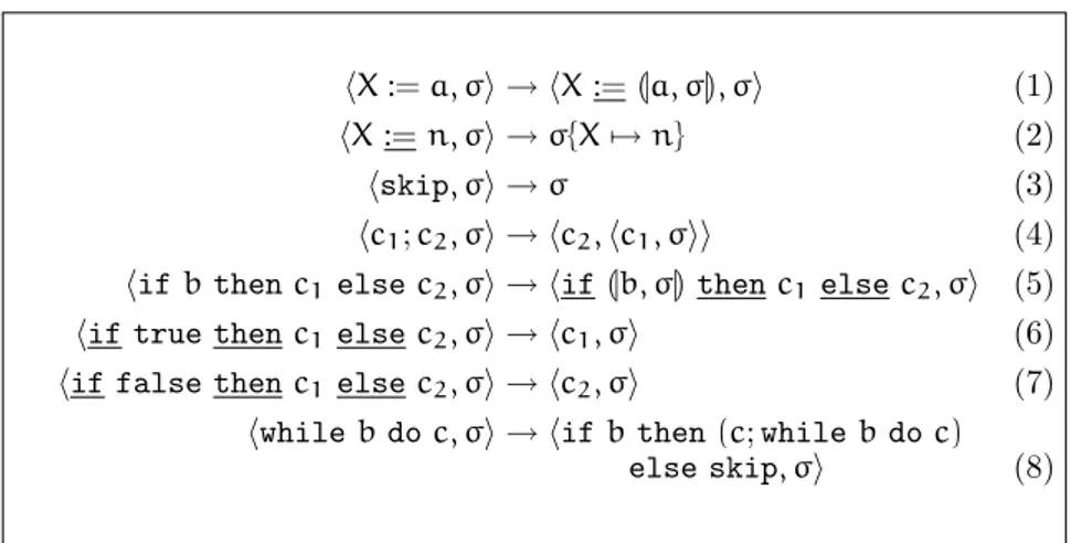
3.1 Evaluation rules for IMP . . . 42
3.2 Big-step semantics for IMP . . . 44
4.1 Semantics of the programming commands . . . 66
4.2 Semantics of the interactive commands. . . 66
4.3 A hardened list strategy . . . 67
6.1 Typing rules for λ1 . . . .. 92
6.2 Typing rules for CIC . . . 95
6.3 The semantics of Coq base tactics . . . 97
6.4 Proof rules for PVS . . . .. 101
6.5 The semantics of PVS base tactics . . . 103
7.1 The semantics of Fellowship’s tactics (1) . . . 116
7.2 The semantics of Fellowship’s tactics (2) . . . 117
7.3 The semantics of Fellowship’s tactics (3) . . . 118
8.1 Two-dimensional operators . . . 129
List of Tables
1.1 Language classes and purposes . . . 15
3.1 Example operational semantics reduction . . . 43 3.2 Example state-based semantics reduction . . . 43
7.1 Concrete notation for L1
m in Fellowship . . . 114
Introduction
An interoperable representation of mathematical proofs can be achieved by combining a simple logical framework with a formal definition of the concept of proof language.
⋆
Formal methods is a discipline at the intersection of mathematics and computer science. It advocates the use of software programs called formal tools to discover, specify and verify the properties of mathematical objects. And since mathematics are the preferred language of experimental sciences such as physics, chemistry or biology, and their engineering derivatives, the range of applications for formal methods is very broad — from verification of spacecraft flight software (Gluck and Holzmann, 2002) to modeling of protein interaction in biological networks (Danos and Laneve, 2004; Eker et al., 2002).
In formal methods, a significant status is given to the objects represent-ing evidence that a given property is verified. For instance, this kind of evidential information is mandatory to pass standardized certification re-quirements, such as the assurance level 7 of the Common Criteria (ISO, 1998), recently adopted as the international standard 15408. The form of the evidence varies, and can be very different from a mathematical proof of the property: some tools just return Ok when the verification is achieved, while others support the generation of a data structure equivalent to a de-tailed mathematical proof.
Proof assistants, or theorem provers1, belong to the second category:
they help the formal methods developer walk through the details of the mathematical proof of a given property, in order to verify it. Modern-day examples of such tools are ACL2, Coq, HOL, Isabelle, Lego, Mizar, NuPrl, PVS, etc. A proof assistant provides a set of commands, or proof language, manipulated by the user to produce a proof, under the supervision of a proof engine ensuring that the user’s operations are mathematically sound. For instance, the proof engine verifies that the specifications input by the user are well-formed, or that a language construct is indeed a description of a mathematically correct proof. Because they already allow their users to deal closely with the proofs during the verification process, usually these tools produce evidence which are close to detailed mathematical proofs.
Still, depending on the proof assistant, the practical form of evidential data is very different. For instance, proofs in PVS are represented by con-structs of the proof language, while in Coq they are objects of the proof term
1
In this manuscript, we consider “theorem prover” as a synonym for “proof assistant”. Historically, theorem provers were fully-automated tools while proof assistants proceeded much more interactively; however the current trend (Boulton, 1992; Aagaard et al., 1993; Lowe and Duncan, 1997) seems to be the convergence of these kinds of systems.
language. What is more, the specification frameworks and proof languages also vary greatly between provers. Combined, these discrepancies are seri-ous enough to impeach the interchangeability, or interoperability, of proofs between tools. As a consequence, if a proof in, e.g. Coq cannot be reused in another prover, then it needs to be re-coded and maintained independently, which is, at best, inefficient. This also limits the opportunities for collabo-rative work between proof developers. Furthermore, as the domain matures, the size of developments grows, amplifying these problems.
As stated earlier, the two main components of a theorem prover are its proof language and its proof engine. In this manuscript, we make the case that interoperability in the representation of proofs can be obtained by enforcing a few conditions on the design of these two components. In par-ticular, we present a simple logical framework, i.e. a base for a proof engine, which checks proofs that are generic enough to fit other proof assistant’s proof engines. We also propose a formalization of the definition of proof languages, which includes the presentation of semantical and typing frame-works, and allow us to better comprehend the existing languages, identify interoperable features, and eventually suggest ways to enhance them.
⋆
Let us spare some words on the topic of proof languages. The concept of proof language was introduced in the s, with the emergence of the first proof assistants: AUTOMATH (de Bruijn, 1970), Mizar (Trybulec, 1978) and Nqthm (Boyer and Moore, 1979, 1988). Most of these used declarative languages, that consist in stating intermediary lemmas until the proof en-gine manages to combine them into the final proof. This approach is quite close to the way proofs are developed in natural language, but does not al-low much interaction between the user and the proof engine. Tools using procedural languages, that provide users with commands to direct the proof engine through the proof construction, appeared almost simultaneously, and blossomed in the following decade: LCF (Gordon et al., 1978, 1979) which can be seen as the ancestor of procedural theorem provers, soon followed by Coq(Coquand and Huet, 1985), NuPrl (Constable et al., 1986), Isabelle (Paulson, 1988), PVS (Owre et al., 1992), HOL (Gordon and Melham, 1993), Lego(Pollack, 1994)), . . . . A detailed comparison of these tools, their logi-cal frameworks and their proof languages, can be found in (Delahaye, 2001; Wiedijk, 2006).
In all these tools, the proof language, be it declarative or procedural, is only a fraction of the complete interaction language of the proof assistant. In addition, there are instructions to specify mathematical objects, a necessary step before starting proving properties on these objects. Depending on the tool reviewed, one can also find instructions enabling modular developments, undo/redo facilities, proof display triggers, etc. A proof language is used solely in proof-editing mode, i.e. the mode entered by the prover when a proof is started, and that the prover leaves when the proof is completed.
On the contrary, the rest of the interaction language can be found in any part of the formal developments. In this work, we are mainly interested in the proof language part of the interaction, and more precisely in procedural proof languages.
Traditionally, elements of proof languages have been divided between tactics and strategies (also called tacticals in some tools), with tactics being used to modify the state of the proof, and strategies being considered as tactics combinators. With time, strategies evolved into an abstraction of the prover’s implementation language, borrowing more and more features from the programming world, and eventually leading to the ML family of programming languages. As a result of this evolution, the exact definition of tactics and strategies is quite vague, and subject to recurring debates. Since these were named after military terms, to examine their meaning in this context does not seem an inappropriate place to start.
The Dictionary of Military and Associated Terms (Uni, 2001) defines tactics as:
“The level of war at which battles and engagements are planned and executed to achieve military objectives.”
And strategies are:
“A prudent idea or set of ideas for employing the instruments of national power in a synchronized and integrated fashion to achieve theater, national, and/or multinational objectives.”
In other terms, tactics are used as a mean to achieve a given local objective: say, prove a particular case of a property. An emphasis is made on the execution of tactics, and they stand close to the action (the construction of the proof) itself. On the contrary, strategies are viewed as a mean to attain a global objective — for example, prove a non-trivial lemma — by devising a way to “synchronize and integrate” tactics.
An atypical definition of the notions of tactics and strategies is given, in a less belligerent context, by theologian and philosopher Michel de Certeau (de Certeau, 1948). De Certeau was interested in the link between human beings and the space they occupy: he links strategies to the design and manipulation of the urban landscape on a high level by institutions and structure of power, and defines tactics as the means employed by individuals to create space for themselves in environments defined by strategies:
“[A tactic is deployed] on and with a terrain imposed on it and organized by the law of a foreign power.”
In this setting, the same idea surfaces: tactics are viewed as fine-grained means to meet an objective in a framework defined by strategies.
In this dissertation, we follow the aforementioned definitions, and we define tactics as procedures that directly modify the proof: the application
of a tactic on a proof in construction extends it. The part of the proof that the tactic applies onto is called the goal, and the extensions generated are called subgoals. Tactics, as transformers of goals into subgoals, thus have a definition that is both operational (i.e. tactics are about execution of the transformation) and local (i.e. tactics are only concerned with one extension of the proof). On the other hand, we view strategies as constructs that take other tactics and strategies as parameters to build a proof. Instantiated strategies, also called proof scripts, derive subgoals from a given goal: they behave just as tactics; however, strategies in their uninstantiated form are inapplicable to proofs, and appear as a way to combine, integrate tactics together. In other terms, we consider strategies as higher-order tactics, i.e. functions on tactics.
Therefore, if it is just a difference between higher and first-order con-structs, is there a need to separate tactics from strategies in a proof lan-guage? Or is it time to reunite the two notions under the unified terminol-ogy of proof commands? In general, we leave this question up for grabs; but for the work exposed here we believe that the distinction between tactics and strategies, if not relevant from an analytical point of view, can still have its utility in the semantical realm. This can be compared to the distinc-tion made in analysis between funcdistinc-tions and constants: the first are just a higher-level version of the second, and having different labels for them helps cope with the mental manipulation of these objects. Hence in the rest of this work, we will try as much as possible to state general properties on proof commands, but we will resort to the tactic / strategies paradigm whenever we feel it aids comprehension. We will also demonstrate how a different take on the classification of proof language constructs can shed a different light on the structure of proof languages.
⋆
Two postulates, originally formulated by de Bruijn as advices to devel-opers of formal tools, guide this work. They can be paraphrased as follows:
Postulate 1 (Simplicity). Strive to keep the underlying for-malism of provers as simple as possible.
Postulate 2(Choice). People will never agree on the logical framework: they need to be given a choice.
Postulate 1 is motivated by both the need to ascertain that at least the core of formal tools is bug-free, supporting the long-standing concept of correctness-by-minimality and the concern that if formal methods are to be popularized, one cannot afford to put off potential users with intricate frame-works and involved theories. Postulate 2 was enacted as a response to the multitude of logical frameworks (in particular with duplication engendered by the classical / intuitionistic schism) that are eligible as a basis for
for-mal tools, and the seemingly never-ending controversy over their respective merits and limitations.
It is easy to see that the two postulates fit tightly the topic of this dissertation: interoperability is, if anything, about choice; and the thesis of this work relies on the elegant simplicity of a logical framework and of a formalism for proof languages. The stake here is in whether both features can be implemented without interference (because in particular, choice hardly entails simplicity), and if the compromises generated with respect to the other parts of the system in order to satisfy postulates 1 and 2 are reasonable.
⋆
The dissertation follows the didactic pattern used in the this introduc-tion. Chapter 1, after a brief recall on predicate languages and sequent calculus, exposes the current state of the art in terms of proof representa-tion. Chapter 2 presents the logical frameworks that are used throughout the rest of the manuscript, and highlights their relations to one another. In chapter 3 to 5 the formalization of the concept of proof language is tackled: chapter 3 draws a parallel between imperative programming languages and procedural proof languages, and sketches a semantical framework for these types of languages; chapter 4 uses a bit of category theory to characterize a pivotal element of the semantics of strategies; chapter 5 provides insights on a typing system for proof languages, and uses the semantical formalism developed in the previous chapters to provide type-safety results.
While first five chapters deal with proof languages in general, and are illustrated using toy examples, the second part of this manuscript instanti-ates these frameworks with concrete proof languages. The chapter 6 builds upon the previous parts to propose a series of methods to achieve interop-erability between proofs in various logical settings, and for various formal tools. Chapter 7 describes an implementation of these ideas on the form of a prototype system for developing interoperable proofs, i.e. an interoperable proof assistant called Fellowship. Finally chapter 8 justifies the viability of the approach taken, by demonstrating a way for first-order logic to finitely express the full power of axiom schemes.
Parts of this dissertation have been published in international confer-ences and workshops (Kirchner, 2005a,b, 2007; Kirchner and Mu˜noz, 2006; Kirchner and Sinot, 2006).
1
Sequent Calculus
This chapter recalls the definition of sequent calculus, exposes some of the means of representing proofs in this formalism, and proposes a classification of proof language constructs.
⋆
First-order logic is a well understood, very widespread formalism. More-over it is quite a capable framework: in practice a lot of real-world spec-ifications and proofs are first-order, and one could argue that in fine the representation of any problem as bits and registers in a computer’s memory is a first-order one. In this manuscript we are interested in a particular logi-cal formalism, where formulas are written in a predicate language and proofs are build using sequent calculus: this chapter presents that formalism. It continues by addressing the topic of the representation of proofs, and finally following up on the discussion of the introduction and proposing a taxonomy for proof language elements.
1.1
Syntax of predicate languages
Definition 1.1.1(L1). Let L1be a language parametrized by the following
possibly infinite, but countable, sets of symbols:
· the set of predicate symbols P = {p, q, . . .}, along with their arities; · the set of function and constant symbols F = {f, g, h . . .}, along with
their arities;
· the set of variable symbols V = {x, y, z, . . .};
The syntax of well-formed terms and formulas of the language follows, in Backus-Naur form:
t, u ::= x | f(t1, . . . , tn)
A, B ::=⊤ | ⊥ | p(t1, . . . , tn)
| ¬A | A⇒ B | A ∧ B | A ∨ B | ∀x.A | ∃x.A
where f and p are respectively function and predicate symbols of arity n, and x is a variable.
Note. The reunion of the sets P and F constitute the signature of L1.
We define informally the main concepts and operations that take place over the language L1— for a formal definition of these mainstream notions,
Bound variables of a formula A are variables appearing in A under the scope of a quantifier on the same variable. Free variables are unbound variables, and fresh variables wrt. a formula A appear neither bound nor free in a A. For instance, in ∀x.p(x, y), x is bound (by the quan-tifier ∀x), y is free and z is fresh.
Substitution is the replacement of a free variable by a term in a term or formula, modulo renaming of variables to avoid variable catching. Substitution is denoted [x ← t]. For instance, (∀x.p(x, y))[y ← f(x)] is ∀z.p(z, f(x)).
Sub-terms and sub-formulas are parts of a term or formula, with free variables possibly substituted. For instance, p(f(x)) is a sub-formula of ∀x.p(x).
The above definition of a predicate language can be adapted to deal with multiple sorts, thus giving rise to many-sorted predicate languages.
Definition 1.1.2 (L1
m). Let L1m be a language comprising:
· a set of sorts S = {s, r, . . .} including a sort bool;
· a set of predicate symbols P = {p, q, . . .}, each with their arity; · a set of function and constant symbols F = {f, g, h, . . .}, each with their
arity;
· for each sort s, a countable set of variables Vs= {x, y, z, . . .}.
Moreover,
· to each function symbol of arity n is associated a rank s1 → . . . →
sn → sn+1 where s1, . . . , sn are the sorts of its arguments and sn+1
is the sort of its result;
· to each predicate symbol p is associated a rank s1→ . . . → sn→ bool
where s1, . . . , sn are the sorts of its arguments;
· for any function or predicate symbol z, we name z∗its associated sort.
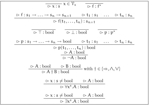
The syntax of well-formed terms and formulas is derived from the syntax of L1, with additional constraints enforced by sorts. This syntax uses Church
notation, where abstractions are decorated with the sorts of their variables. The well-formedness constraints are given using inference rules to reflect the conditional nature of their formulation: for instance, a term f(t1, . . . , tn)is
well-formed if f is a function symbol of rank s1→ . . . → sn → sn+1, and
each ti has sort si. Using the notation 3 a : s for the statement “a is a
well-formed term or formula of sort s”, figure 1.1 presents the inference rules for well-formed terms and formulas.
Note. This is a slight variation in notation from the common presentation of many-sorted first-order languages, where ranks are written using tuples instead of arrows, and for predicates the final sort bool is omitted.
x∈ Vs 3 x : s 3 f : f∗ 3 f : s1→ . . . → sn→ sn+1 3 t1: s1 . . . 3 tn : sn 3 f(t1, . . . , tn) : sn+1 3 ⊤ : bool 3 ⊥ : bool 3 p : p∗ 3 p : s1→ . . . → sn→ bool 3 t1: s1 . . . 3 tn: sn 3 p(t1, . . . , tn) : bool 3 A : bool 3 ¬A : bool
3 A : bool 3 B : bool with † ∈ {⇒, ∧, ∨} 3 A † B : bool
3 x : s 6= bool 3 A : bool 3 ∀xs.A : bool
3 x : s 6= bool 3 A : bool 3 ∃xs.A : bool
Figure 1.1: Syntax of well-formed terms and formulas in L1 m
Notation. Contiguous universal and existential quantifications over similarly-sorted variables are collapsed. For instance, the formula ∀xs
1.(. . . (∀xsn.A))
is written ∀x1, . . . , xsn.A.
All other concepts, such as bound and free variables, replacement, sub-stitution, sub-terms and sub-formulas, are extended similarly to deal with many-sorted terms and formulas.
1.2
The sequent calculus
Sequent calculus is a logical formalism pioneered by Gentzen in 1935, orig-inally as a tool to study natural deduction (Gentzen, 1935). As with any calculus, it has two fundamental components: objects called sequents, and some sort of computation called deduction.
Sequents assert that from a finite multiset of formulas Γ , one can prove at least a formula of another multiset ∆. This assertion is noted Γ ⊢ ∆, and Γ and ∆ are called respectively the antecedent and the succedent. Unlike in the Gentzen’s presentation of sequents, we make it possible to distinguish a particular formula amongst the members of Γ and ∆, called active formula. Depending if an active formula A belongs to the antecedent or the succedent of a sequent, we note Γ ; A ⊢ ∆ or Γ ⊢ A; ∆: we say that such a sequent is polarized.
Deduction consists in a series of rules, that transform an input sequent into zero, one or more resulting sequents. These transformations are called inferences, and denoted by the vertical stacking of input and output sequents, separated by a horizontal bar and annotated with the name of the rule. For instance, is S0 is the input sequent and
S1, . . . , Sn are the output sequents of a rule r, we write:
S1 . . . Sn
r
S0
In particular, if the input sequent contains an active formula, only this formula is subject to a computation, i.e. its non-active parts will be found unchanged by the inference in the output sequents. Rules that deal with an active formula are earmarked with either a left labelLor
a right labelR, depending on the polarization of the sequent.
When a sequent calculus is defined based on a first-order predicate lan-guage such as the ones of definitions 1.1.1 and 1.1.2, it forms a logical frame-work called first-order logic.
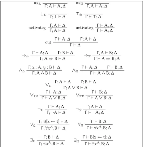
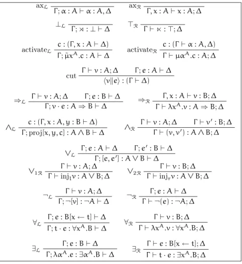
Definition 1.2.1 (lkµ ˜µ). Figure 1.2 presents a set of inference rules that
define a classical sequent calculus called lkµ ˜µ (Herbelin, 2005), based on
the single-sorted predicate language L1.
Remark that because we use a definition of sequents where the antecedent and the succedent are multisets, there is no need in this system for formula-swapping rules. The weakening rules are moved into the axiom rules, and contraction rules are missing from the figure 1.2. One can chose either to add them directly, resulting in two new inference rules. The alternative is to encode them using the cut rule with a notable drawback: the cut-elimination property no longer holds, simply because contraction cannot be eliminated without losing logical completeness.
1.3
Proofs and traces
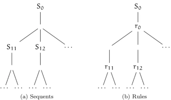
A proof consists of a series of computations over an initial input sequent, by successive application of rules: when no output sequent remains, the initial sequent is proved. The trace of the computation is often stored for future reference, in the form of a tree of sequents where edges are labelled by rules, often called proof tree. Figure 1.3 illustrates the form of a trace.
Notice however that there is some redundancy in this representation, because inference rules are deterministic. For instance in lkµ ˜µ, if an input
sequent Γ ; A ⇒ B ⊢ ∆ produces two sequents Γ ⊢ A; ∆ and Γ ; B ⊢ ∆, then we know that only the ⇒L rule can have resulted in that transformation.
Hence the information contained in the tree of sequents is enough to build a complete representation of a proof.
axL Γ ; A⊢ A, ∆ axR Γ, A⊢ A; ∆ ⊥L Γ ;⊥ ⊢ ∆ ⊤R Γ ⊢ ⊤; ∆ Γ, A⊢ ∆ activateL Γ ; A⊢ ∆ Γ ⊢ A, ∆ activateR Γ ⊢ A; ∆ Γ ⊢ A; ∆ Γ ; A⊢ ∆ cut Γ ⊢ ∆ Γ ⊢ A; ∆ Γ ; B⊢ ∆ ⇒L Γ ; A⇒ B ⊢ ∆ Γ, A⊢ B; ∆ ⇒R Γ ⊢ A ⇒ B; ∆ Γ, x : A, y : B⊢ ∆ ∧L Γ ; A ∧ B⊢ ∆ Γ ⊢ A; ∆ Γ ⊢ B; ∆ ∧R Γ ⊢ A ∧ B; ∆ Γ ; A⊢ ∆ Γ ; B⊢ ∆ ∨L Γ ; A ∨ B⊢ ∆ Γ ⊢ A; ∆ ∨1R Γ ⊢ A ∨ B; ∆ Γ ⊢ B; ∆ ∨2R Γ ⊢ A ∨ B; ∆ Γ ⊢ A; ∆ ¬L Γ ; ¬A⊢ ∆ Γ ; A⊢ ∆ ¬R Γ ⊢ ¬A; ∆ Γ ; B[x← t] ⊢ ∆ ∀L Γ ;∀xA.B⊢ ∆ Γ ⊢ B; ∆ ∀R Γ ⊢ ∀xA.B; ∆ Γ ; B⊢ ∆ ∃L Γ ;∃αA.B⊢ ∆ Γ ⊢ B[x ← t]; ∆ ∃R Γ ⊢ ∃xA.B; ∆
Figure 1.2: Inference rules for lkµ ˜µ
S0 r0 S11 r11 . . . . S12 r12 . . . . . . .
S0 S11 . . . . S12 . . . . . . . (a) Sequents S0 r0 r11 . . . . r12 . . . . . . . (b) Rules
Figure 1.4: Non redundant proof traces
Conversely, if given an input sequent and an inference rule, then one can deduct the result sequents. By induction, one can reconstitute the complete proof representation from only the initial sequent and the collection of infer-ence rules. The two simplified representations are summarized in figure 1.4.
However, proofs can become large objects, taking even sometimes years to develop (Hales, 2004; Gonthier, 2005). Therefore, there is a need to store and represent proofs in the making, i.e. open proofs. In these proofs, one or more sequents are left untouched by inference rules: they are called open goals; any part of the proof tree that contains at least one open goal is called an open branch. Dealing with these open proofs is not a problem in the representation of figure 1.4a: the unproved sequents will just be leaves of the tree (sometimes emphasized by using a question mark above them). However, in the representation of figures 1.3 and 1.4b, there is a need for a new inference rule, stating that the associated sequents are unproved. To this end, we introduce the idtac rule, which is the identity computation, i.e. processes its input sequent into the same output sequent. This rule acts as a placeholder for another inference, allowing for well-formed trace trees.
1.4
A taxonomy of proof commands
Now that the logical framework has been defined, and that the topic of proof representation has been evoked, we can complete the discussion started in the introduction about the classification of proof language constructs.
In modern procedural theorem provers, some tactics correspond to the bare logical inference rules, while others are abstracted and automated ver-sions of these rules. When building a proof, both kinds of tactics are used, but when available the latter is often preferred, because of their ease of use
— the advantages they provide to facilitate the interactive process range from automatic name generation to complex backtracking and branching features.
What is more, proofs are seldom saved in their canonical, tree-like form. Instead, what is retained is the proof script that generated them. While this kind of representation has the advantage of giving a higher-level (albeit unstructured) comprehension of the essence of the proof and facilitating its re-edition, it also has the flaw of being easily broken by changes in the proof language semantics. In some cases, the tactics may be over-dimensioned for the goal, and thus provide very few information to the reader. For instance, calling an automatic first-order solver via a tactic on a first-order goal masks the effective inference rules and forces the reader looking for a finer-grained proof to re-discover it.
We argue that these two pattern of utilisation for proof languages are equally important in their uses. Hence in establishing a classification of such languages, we will consider the following criterions:
1. Is the language construct used to build the proof? 2. Is the language construct suitable to represent the proof?
Commands as inference rules
The first identifiable set of commands corresponds to the tactics that imple-ment the logical framework’s inference rules. The presence of these tactics is by definition a requisite for procedural theorem proving, and they constitute the building bricks of the proof. As such, they are mandatory both to build a proof and its representation. We call them base tactics.
Commands as programming constructs
Strategies are used to build other commands, i.e. they act as a programming language at the level of the proof language. They are not used directly to construct proofs per se, but rather to build the proof builders. Moreover, strategies are not suited for the representation of proofs. Indeed, because they are in essence programming constructs, only the result of the programs are to be retained. As an example, take the following proof script:
try (apply lemma_1) (apply lemma_2)
that attempts to perform a deduction by applying the result of a first lemma, and that applies a second lemma if the first one is unsuccessful. Whichever branch of the try strategy gets selected should be recorded in the represen-tation of the proof. However, there is no point in recording the whole script. We call these programming strategies.
Yet there are two constructs that are important exceptions to the non representativity of strategies:
· ;[||], which combines commands in a tree structure, isomorphic to the structure of the proof. It is the “glue” that holds the building bricks of the proof together, and thus it is necessary to the representation of non-trivial proofs.
· idtac, that “does nothing” when applied to a sequent. It is used to represent incomplete proofs, and fill the place where later tactics might be added.
Together with tactics, these two strategies are all that are needed to repre-sent proofs. In reference to their tree-structuring functionality, we call these special programming strategies bark strategies.
Commands as super inference rules
We call extended tactic a command that is defined as a combination of tactics, by either using strategies or the prover’s implementation language. Thus an extended tactic may be seen as a super inference rule, created by the combination of smaller rules. As such, extended tactics are proof builders, on par with base tactics.
At the level of proof representation, extended tactics should be viewed as labelled boxes containing instances of inference rules. Or, equivalently, a combination of base tactics and bark strategies. This enables the proof reader to eventually refine its understanding of the proof by “opening the box” labelled by an extended tactic. For instance, the apply tactic men-tioned in the previous paragraph should be expandable to display the ap-propriate cut rule, and the quantifier rules that have been used to achieve unification.
Commands as interaction controls
Building a proof is a largely interactive process, with goals being presented one by one, postponed, changes undone, etc.. The last group of commands are the ones that control such interactions. They do not contribute directly to the construction of the proof, neither should they appear in a finished proof script. Examples of such commands include the postpone construct evoked in the introduction, PVS’s (hide) / (reveal) or Coq’s focus. Also, Coq’s unassuming ‘.’ command, that (literally) punctuates command ap-plications, should be seen as both an evaluation trigger and an interactive control, returning the first subgoal of the active subtree once the evaluation is complete. We call these controls interactive commands.
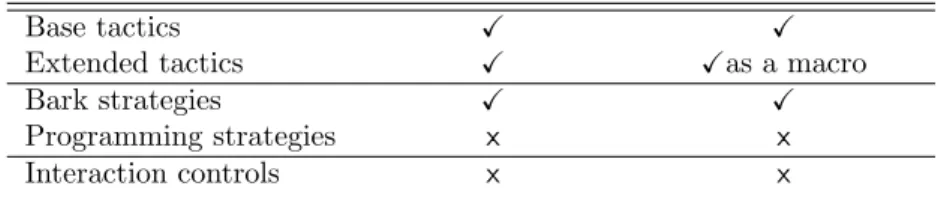
Table 1.1 sums up the behaviour of the different language classes with respect to these two criterions.
Table 1.1: Language classes and purposes
Proof construction Proof representation
Base tactics X X
Extended tactics X Xas a macro
Bark strategies X X
Programming strategies x x
2
¯λµ˜µ-Calculus and Variations
Here we define the logical framework of our developments, in the form of a proof term calculus; it is declined into four variations: classical, intuitionis-tic, and their respective minimal weakening.
These frameworks are adaptations of the system lkµ ˜µ, defined in
chap-ter 1, that present inchap-teresting characchap-teristics for inchap-teractive theorem proving and proof interoperability. What is more, the simplicity and diversity of the first-order logics they define qualifies them under both postulates 1 and 2.
In this chapter we review the principle of the proof-as-term isomorphism, illustrated with the example of the lkµ ˜µsystem. Then, by the means of this
isomorphism, we detail the logical inference rules of our original systems; we start with the most general logical setting, i.e. classical logic, and from there we work our way through more restricted, intuitionistic and minimal, settings. We conclude with the representation of incomplete proofs.
⋆
The Curry-de Bruijn-Howard correspondence identifies formulas as types, making a sequent into a typing statement, and deduction rules as type in-ferences. The objects being typed are called proof terms, which should not be confused with terms of the predicate language (to this end, we will never omit the ‘proof’ adjective when referring to proof terms). For instance, a well-known proof term language is the λ-calculus, which can label formulas of minimal natural deduction.
Classical sequent calculus being a more elaborate construction than min-imal natural deduction, the proof term language also needs to be more com-plex than plain λ-calculus. A few languages have been proposed, from Her-belin’s ¯λ-calculus (Herbelin, 1995) to Urban’s calculus of names and conames (Urban, 2001), and including Girard’s ?, and Barbarena and Berardi’s ? cal-culi. In all of these formalisms, the idea is to associate with each inference rule a construction of the proof term language.
Along with the choice of a proof language, one needs to examine to fol-lowing question: to which element of the sequent is a proof term associated? The problem of the place of the proof term in the sequent arises because, unlike in natural deduction, a deduction in sequent calculus can take place on any formula in a sequent. The use of sequents with active formulas partly solve this question: the polarization marks the target of the computation. The active formula in a sequent is considered as the type of a particular proof term (independently from the choice of a proof term language). Thus sequents are written:
However in case where there is no active formula, the problem remains. The solution is to have the whole sequent represent the type of the proof term, which we note:
t : (Γ ⊢ ∆)
Interestingly, this last notation is not much different from the one proposed by Urban, where the proof term is a component of the sequent, at the same level as the antecedent or the succedent.
In the rest of this chapter, we introduce ¯λµ˜µ, a calculus of proof terms that works with sequents that have active formulas. This presentation uses the flip side of the Curry-de Bruijn-Howard correspondence: we define a calculus of proof terms as a labeling system for a given logical framework, instead of defining the logics as a type inference system for a particular language. Of course, an isomorphism being symmetrical by nature, it is sometimes easier to refer to the typing side of the correspondence. The logical aspects, however, will remain the guiding concern of this development.
2.1
The proof-as-term isomorphism for lk
µ ˜µFor the deduction system lkµ ˜µ, the proof language used by Herbelin is
called the ¯λµ˜µ-calculus (Curien and Herbelin, 2000; Wadler, 2003; Herbelin, 2005), i.e. an extension of λ-calculus with two binders µ and ˜µ to capture classical logic, and the choice of an active formula in the sequent. What is more, one introduces additional operators to reflect the types ∧ and ∨, and a symmetrical to λ to inhabit existential types.
Note that because our purpose is only to give a quick overview of the mechanisms of the calculus, we do not enter its details. All these results can be found and further explained in (Curien and Herbelin, 2000; Herbelin, 2005).
Definition 2.1.1(¯λµ˜µproof terms). The syntax of the ¯λµ˜µ-calculus defines commands c, terms v and environments e:
c ::=hvkei
v, v′::= x | ⋉ | λxA.v | e· v | ¬(e) | (v, v′) | injrv | injlv | µαA.c e, e′::= α | ⋊ | v· e | ˜λαA.e | ¬[v] | proj[x, x′, c] | [e, e′] | ˜µxA.c
where A is a formula. ⋉ and ⋊ are constants, respectively called unit and tinu, linked to the connectors ⊤ and ⊥.
Remark that this syntax is perfectly symmetrical, notwithstanding the projection operators (due to lkµ ˜µ’s asymmetric use of an additive sum and
of a multiplicative product). The symmetry is extended to the reduction rules of the calculus.
Definition 2.1.2(Reduction rules for ¯λµ˜µ). The evaluation rules for ¯λµ˜µ proof terms are the same as in (Curien and Herbelin, 2000): one will recog-nize the evaluation relations for λ, µ and ˜µ redexes, enriched with the dual projection and pair reductions.
hλxA.v1kv2· ei → hv2k˜µxA.hv1keii (λ)
h(e2· v)k˜λβA.e1i → hµβA.hvke1ike2i (˜λ)
hµβA.ckei → c[β ← e] (µ)
hvk˜µxA.ci → c[x ← v] (˜µ) hinjlvk[e1, e2]i → hvke1i (injl)
hinjrvk[e1, e2]i → hvke2i (injr)
h(v1, v2)kproj[x1, x2, c]i → hv1k˜µx1.hv2k˜µx2.cii (proj1)
h(v1, v2)kproj[x1, x2, c]i → hv2k˜µx2.hv1k˜µx1.cii (proj2)
Note. Let us recall a few customary observations: first of all notice that the rules (µ) and (˜µ) one the one hand, and (λ) and (˜λ) on the other hand, are dual from one another. Second, notice that the rules (µ) and (˜µ) form a critical pair, and that giving priority to the first reduction imposes a value reduction strategy, whereas the alternative results in a call-by-name reduction strategy. Note that the rules (proj1) and (proj2) also form
a critical pair, convergent in the case of a call-by-name strategy but not so for call-by-value.
Definition 2.1.3 (Equivalence rules for ¯λµ˜µ). A series of η-equivalences can be defined for each of the binders in the proof term syntax:
v↔ λx.µα.hvkx · αi x, αnot free in v (ηR λ)
e↔ µβ.hλx.µα.hxkβikei · ˜µy.hλx.ykei βnot free in e (ηL λ)
v↔ ˜µy.hvk˜λα.˜µx.hykαii · µβ.hvk˜λα.βi ynot free in v (ηR ˜ λ)
e↔ ˜λα.˜µx.hα · xkei αnot free in e (ηL ˜λ)
v↔ µα.hvkαi αnot free in v (ηµ)
e↔ ˜µx.hxkei xnot free in e (ηµ˜)
And for the projection and pair operators:
v↔ (µα.hvkπ1(α)i, µβ.hvkπ2(β)i) (ηRproj)
e↔ ˜µz.hzkπ1(˜µx.hzkπ2(˜µy.h(x, y)kαi)ii) (ηL1proj)
e↔ ˜µz.hzkπ2(˜µy.hzkπ1(˜µx.h(x, y)kαi)ii) (ηL2proj)
v↔ µα.hinjlµβ.hinjrµγ.[β, γ]kαikαi (ηL1inj)
v↔ µα.hinjrµγ.hinjlµβ.[β, γ]kαikαi (ηL2inj)
assuming the following definitions:
π1(e) = proj[x1, x2,hx1kei]
π2(e) = proj[x1, x2,hx2kei]
The definition of the notion of linearity on ¯λµ˜µ proof terms is a bit stronger than the usual definition of linearity: it implies that binder of linear variables do no overlap.
Definition 2.1.4(Linearly bound variables). In a proof term t, we say that a variable x is bound linearly by a binder b (either λ, µ or ˜µ) in a subterm uif:
· xis bound by b in u, · xappears exactly once in u,
· between b and x, there is no occurrence of a binder of the same kind as b.
As highlighted in the introducing paragraph, typing statements for ¯λµ˜µ proof terms, i.e. sequents in the logical formalism, are of the three following forms:
Γ ; e : A⊢ ∆ Γ ⊢ v : A; ∆ c : (Γ⊢ ∆)
where A is a formula of L1
m, and the contexts Γ and ∆ are multisets of labeled
formulas of L1
m. By using multisets instead of plain lists, formula-swapping
rules are made implicit.
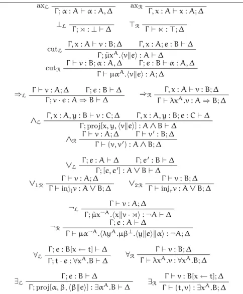
Definition 2.1.5. Figure 2.1 presents the logical system lkµ ˜µ and a set of
type inference rules for ¯λµ˜µ.
Note. In figure 2.1, the usual quantifier side conditions have been omitted for space : in ∀R (resp. ∃L), the variable x (resp α) does not appear free
in Γ or ∆; in ∀L and ∃R, t and x have the same sort A. This leads us to
another remark: an implicit conversion is done between sorts and formulas for the bound variables of the quantifier rules. Because of the trivial injection between ranking system and the formulas of first-order logic, this coercion works as expected.
Figure 1.2 does not include formula management rules, which are pre-sented here. There are four weakening rules:
Γ ⊢ v : C; ∆ weak1R Γ, x : A⊢ v : C; ∆ Γ ⊢ v : C; ∆ weak2R Γ ⊢ v : C; x : A, ∆ Γ ; e : C⊢ ∆ weak3L Γ, x : A; e : C⊢ ∆ Γ ; e : C⊢ ∆ weak4L Γ ; e : C⊢ x : A, ∆
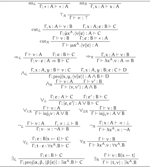
axL Γ ; α : A⊢ α : A, ∆ axR Γ, x : A⊢ x : A; ∆ ⊥L Γ ; ⋊ :⊥ ⊢ ∆ ⊤R Γ ⊢ ⋉ : ⊤; ∆ c : (Γ, x : A⊢ ∆) activateL Γ ; ˜µxA.c : A⊢ ∆ c : (Γ ⊢ α : A, ∆) activateR Γ ⊢ µαA.c : A; ∆ Γ ⊢ v : A; ∆ Γ ; e : A⊢ ∆ cut hvkei : (Γ ⊢ ∆) Γ ⊢ v : A; ∆ Γ ; e : B⊢ ∆ ⇒L Γ ; v· e : A ⇒ B ⊢ ∆ Γ, x : A⊢ v : B; ∆ ⇒R Γ ⊢ λxA.v : A⇒ B; ∆ c : (Γ, x : A, y : B⊢ ∆) ∧L Γ ; proj[x, y, c] : A ∧ B⊢ ∆ Γ ⊢ v : A; ∆ Γ ⊢ v′: B; ∆ ∧R Γ ⊢ (v, v′) : A ∧ B; ∆ Γ ; e : A⊢ ∆ Γ ; e′: B⊢ ∆ ∨L Γ ; [e, e′] : A ∨ B⊢ ∆ Γ ⊢ v : A; ∆ ∨1R Γ ⊢ injlv : A ∨ B; ∆ Γ ⊢ v : B; ∆ ∨2R Γ ⊢ injrv : A ∨ B; ∆ Γ ⊢ v : A; ∆ ¬L Γ ; ¬[v] : ¬A⊢ ∆ Γ ; e : A⊢ ∆ ¬R Γ ⊢ ¬(e) : ¬A; ∆ Γ ; e : B[x← t] ⊢ ∆ ∀L Γ ; t· e : ∀xA.B⊢ ∆ Γ ⊢ v : B; ∆ ∀R Γ ⊢ λxA.v :∀xA.B; ∆ Γ ; e : B⊢ ∆ ∃L Γ ; λαA.e :∃αA.B⊢ ∆ Γ ⊢ e : B[x ← t]; ∆ ∃R Γ ⊢ t · e : ∃xA.B; ∆
Figure 2.1: lkµ ˜µas a type inference system for ¯λµ˜µ
and the two contraction rules are derived using cut and axiom rules.
Γ ⊢ v : C; α : C, ∆ contrR Γ ⊢ µαC.hvkαi : C; ∆ Γ, x : C; e : C⊢ ∆ contrL Γ ; ˜µxC.hxkei : C ⊢ ∆
Note. This system does not have the cut-elimination property, because it makes use of the cut rule to encode contraction.
Remark that once a formalism for introducing proof terms in sequents is devised, the notion of deductive computation can be replaced by one of type inference of a proof term. Because the whole proof trace can be replaced by a proof term, the proof-as-term morphism offers a compact alternative to
the representations of figures 1.3 and 1.4. For instance, the ¯λµ˜µproof term:
λxA.λyA⇒B.µαB.hykx · αi
when typechecked in the system lkµ ˜µ, builds a proof of the tautology A ⇒
(A⇒ B) ⇒ B.
In the following sections we propose a series of original logical systems derived from lkµ ˜µ. We will see how they are adapted to interactive proof
construction, and overall proof manipulation.
2.2
The classical system lk
Proof terms for our classical framework lk are expressed in a slight sim-plification of the ¯λµ˜µ-calculus, arguably better-suited for interactive proof construction. In the rest of this manuscript, we use the name ¯λµ˜µ to des-ignate this simplification. We give first the syntax of the calculus, before developing the reduction rules.
Definition 2.2.1 (Simpler ¯λµ˜µproof terms). The simplified syntax of the ¯
λµ˜µ-calculus defines commands c, terms v and environments e:
c ::=hvkei
v, v′::= x | ⋉ | λxA.v | (v, v′) | injrv | injlv | µαA.c e, e′::= α | ⋊ | v· e | proj[x, x′, c] | [e, e′] | ˜µxA.c
This syntax is similar to the one of definition 2.1.1, with the environment constructors λ and ¬ and the term constructors · and ¬ removed.
Definition 2.2.2(Reduction and equivalence rules for ¯λµ˜µ). Following the restriction in the syntax, the reduction rules (˜λ), (ηR
˜
λ) and (η L ˜
λ) are discarded.
All other rules from definitions 2.1.2 and 2.1.3 are applicable to the restricted ¯
λµ˜µ proof terms.
Typing statements for ¯λµ˜µproof terms, i.e. sequents in the logical for-malism, are of the two following forms:
Γ ; e : A⊢ ∆ Γ ⊢ v : A; ∆
where the contexts Γ and ∆ are multisets of labeled formulas — by using multisets instead of plain lists, formula-swapping rules are made implicit. Contrary to lkµ ˜µ, remark the absence of any judgements without active
formula, i.e. of the form c : (Γ ⊢ ∆).
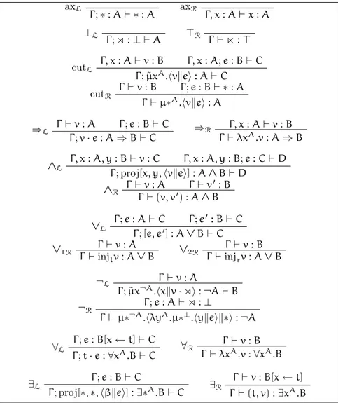
Definition 2.2.3 (lk). Figure 2.2 describes the logical inference rules for first-order classical sequent calculus. This system is called lk.
axL Γ ; α : A⊢ α : A, ∆ axR Γ, x : A⊢ x : A; ∆ ⊥L Γ ; ⋊ :⊥ ⊢ ∆ ⊤R Γ ⊢ ⋉ : ⊤; ∆ Γ, x : A⊢ v : B; ∆ Γ, x : A; e : B⊢ ∆ cutL Γ ; ˜µxA.hvkei : A ⊢ ∆ Γ ⊢ v : B; α : A, ∆ Γ ; e : B⊢ α : A, ∆ cutR Γ ⊢ µαA.hvkei : A; ∆ Γ ⊢ v : A; ∆ Γ ; e : B⊢ ∆ ⇒L Γ ; v· e : A ⇒ B ⊢ ∆ Γ, x : A⊢ v : B; ∆ ⇒R Γ ⊢ λxA.v : A⇒ B; ∆ Γ, x : A, y : B⊢ v : C; ∆ Γ, x : A, y : B; e : C⊢ ∆ ∧L Γ ; proj[x, y,hvkei] : A ∧ B ⊢ ∆ Γ ⊢ v : A; ∆ Γ ⊢ v′ : B; ∆ ∧R Γ ⊢ (v, v′) : A ∧ B; ∆ Γ ; e : A⊢ ∆ Γ ; e′: B⊢ ∆ ∨L Γ ; [e, e′] : A ∨ B⊢ ∆ Γ ⊢ v : A; ∆ ∨1R Γ ⊢ injlv : A ∨ B; ∆ Γ ⊢ v : B; ∆ ∨2R Γ ⊢ injrv : A ∨ B; ∆ Γ ⊢ v : A; ∆ ¬L
Γ ; ˜µx¬A.hxkv · ⋊i : ¬A ⊢ ∆
Γ ; e : A⊢ ∆ ¬R
Γ ⊢ µα¬A.hλyA.µβ⊥.hykeikαi : ¬A; ∆
Γ ; e : B[x← t] ⊢ ∆ ∀L Γ ; t· e : ∀xA.B⊢ ∆ Γ ⊢ v : B; ∆ ∀R Γ ⊢ λxA.v :∀xA.B; ∆ Γ ; e : B⊢ ∆ ∃L Γ ; proj[α, β,hβkei] : ∃αA.B⊢ ∆ Γ ⊢ v : B[x ← t]; ∆ ∃R Γ ⊢ (t, v) : ∃xA.B; ∆
Definition 2.2.4. A classical proof term is an expression of ¯λµ˜µ that is well-typed in the system of figure 2.2.
A general remark on the lk logical system is that it retains as much information as possible: in particular, formulas are duplicated in order to forego destructive inferences. More precisely, in this framework:
· the contraction rule is embedded into much of the inferences: in bottom-up application of inferences, when branching is achieved, the contexts in both hypothesis and conclusion are duplicated. Hence ∨L and ∧R
are additive rules, while ∧L uses the inference for multiplicative
con-junction. Incidentally, for the sake of symmetry, a cut rule is embedded in the ∧Lrule, the alternatives (having two inference rules depending
on which formula is focussed upon, or arbitrarily choosing A or B as the principal formula for the rule’s hypothesis) being deemed unsatis-factory. Finally, the choice of an additive ∨R rule is a minor deviation
from the aforementioned principle, justified by the coherence with the intuitionistic fragment of this formalism, detailed later. Moreover, the right rule for a multiplicative disjunction is easily simulated using a cut.
· these choices have an impact on the quantifiers side. While the pendent product ∀ is unsurprisingly labeled by a λ construct, the de-pendent sum ∃ reuses the environment projection operator, instead of introducing a new notation as it is the case in lkµ ˜µ. This is made
possible by the multiplicativity of the ∧Lrule, which in turn produced
a projection constructor rich enough to label the existential quantifier rule.
· (ηµ) and (ηµ˜) expansions are used to explicitly store the type of a ¯λµ˜µ
expression inside a η-redex. For instance, if v is a term of type A, one can record this type information using a variable α by performing the following (ηµ) expansion:
v→ µαA.hvkαi
This is used in the case of the deduction rules for negation ¬Rand ¬L,
to generate non-minimal proof terms that include information about the expansion of negation into an implication. A (ηµ) expansion is
also performed at the beginning of each proof, in order to store in the proof term the formula that is being proven.
These characteristics make the system lk well-suited for interactive theorem proving and proof interoperability, two topics that require proof structures as information-rich as possible.
In lk, since there are no typing judgements for standalone commands, they are typed only as subterms of a term or a environment. In short, this consists in a variation of lkµ ˜µ, inlining the ‘cut’ and ‘activate’ rules into
any rule that produces a command. Thus the rules for cutR, cutL, ∧L and
∃L. A consequence of this design is the following proposition.
Proposition 2.2.5(Liveliness). For any sequent in a lk proof, there is an active formula.
Proof. By induction on the structure of the proof.
The liveliness property is important to us for several reasons, related to the practice of interactive proof systems. First, it is essential to ensure that the user of such systems always knows which formula he is working on. Having sequents where there are distinguished formulas, and others where there are none, arguably adds a level of complexity to the (already involved) comprehension and intuition of a proof formalism. Second, in the case of automated or partly-automated theorem proving, it is conjectured that this property facilitates the design of algorithms, and reduces the search space: this intuition is also mentioned in (Sacerdoti Coen, 2006), and works by Andreoli (Andreoli, 1992) and more recently Saurin (Saurin, 2006) on focussing proofs tend to confirm this hypothesis.
The formula management rules for lk (weakening and contraction) are similar the corresponding rules of lkµ ˜µ.
Proposition 2.2.6. The logical system lk is equivalent to the lkµ ˜µ
formu-lation of first-order classical sequent calculus, as per definition 1.2.1.
Proof. The equivalence between L1 and L1
m, i.e. single-sorted and
many-sorted first-order languages, is an established result. A many-many-sorted lan-guage can be encoded in a single-sorted lanlan-guage by introducing predicate symbols that represent sort membership. On the logical side, when consid-ering unannotated formulas, the system lk is similar to lkµ ˜µexcept for the
cut and left conjunction:
· the cutL and cutR are inlined versions of the usual focus and cut
inference rules. The equivalence holds because in lkµ ˜µ, the only rule
that can follow a focus on the left or on the right is a cut rule. · the same reasoning holds for the left conjunction rule ∧L. While
embedding a focus rule would have been sufficient, the use of an addi-tional cut rule is not detrimental to the equivalence of both systems, as choosing C = A or C = B and using the weakening rules proves.
The labelling of the proofs by proof terms is slightly different in lk and in lkµ ˜µ. It is easy, by using typing information in some cases, to establish a
translation between them. In particular, the two symbols ¬ and the left λ in lkµ ˜µ are equivalent to constructions using ·, λ and proj in lk.
Proof. This follows from proposition 2.2.6, i.e. equivalence with Herbelin’s lkµ ˜µ sequent calculus.
Note. As in lkµ ˜µ, cut elimination in lk is lost to compound contraction
rules.
2.3
The intuitionistic system lj
Restricting the framework of classical logic to an intuitionistic formalism is a simple process: it suffices to constrain the conclusion of sequents to contain at most one formula. This constraint has a clearly identifiable counterpart at the proof term level. Indeed, when introducing a µ-abstraction to name the formula one wants to prove next, the previously designated formula and its label are overridden, due to the one-formula-per-consequent constraint. As a consequence, only one environment variable, denoted ∗, is ever used, and the µ-bindings do not overlap: the environment variables for intuitionistic proof terms are linearly bound.
Definition 2.3.1 (¯λµ˜∗µ proof terms). The ¯λµ˜∗µ terms are similar to ¯λµ˜µ terms, albeit with a unique environment variable ∗.
c ::=hvkei
v, v′::= x | ⋉ | λxA.v | (v, v′) | injrv | injlv | µ∗A.c e, e′::=∗ | ⋊ | v · e | proj[x, x′, c] | [e, e′] | ˜µxA.c
The reduction rules given in definition 2.2.2, with the relevant cases pruned, still hold. Also, the form of the typing statements for proof terms isn’t changed from section 2.2.
The one formula limitation entails the deprecation of the right contrac-tion rule contrR and the right weakening rule weak2R. Only remain the
following weakening and contraction rules: Γ ⊢ v : C weak1R Γ, x : A⊢ v : C Γ, x : C; e : C⊢ y : D contrL Γ ; ˜µxC.hxkei : C ⊢ y : D Γ ; e : C⊢ y : D weak3L Γ, x : A; e : C⊢ y : D Γ ; e : C⊢ weak4L Γ ; e : C⊢ x : A
Definition 2.3.2(lj). Figure 2.3 exposes the inference rules for first-order intuitionistic sequent calculus.
Definition 2.3.3. An intuitionistic proof term is an expression of ¯λµ˜∗µthat is well-typed in the system of figure 2.3.
The intuitionistic formalism being a weakened version of the classical setting, it inherits its liveliness property (proposition 2.2.5).
axL Γ ;∗ : A ⊢ ∗ : A axR Γ, x : A⊢ x : A ⊥L Γ ; ⋊ :⊥ ⊢ A ⊤R Γ ⊢ ⋉ : ⊤ Γ, x : A⊢ v : B Γ, x : A; e : B⊢ C cutL Γ ; ˜µxA.hvkei : A ⊢ C Γ ⊢ v : B Γ ; e : B⊢ ∗ : A cutR Γ ⊢ µ∗A.hvkei : A Γ ⊢ v : A Γ ; e : B⊢ C ⇒L Γ ; v· e : A ⇒ B ⊢ C Γ, x : A⊢ v : B ⇒R Γ ⊢ λxA.v : A⇒ B Γ, x : A, y : B⊢ v : C Γ, x : A, y : B; e : C⊢ D ∧L Γ ; proj[x, y,hvkei] : A ∧ B ⊢ D Γ ⊢ v : A Γ ⊢ v′ : B ∧R Γ ⊢ (v, v′) : A ∧ B Γ ; e : A⊢ C Γ ; e′: B⊢ C ∨L Γ ; [e, e′] : A ∨ B⊢ C Γ ⊢ v : A ∨1R Γ ⊢ injlv : A ∨ B Γ ⊢ v : B ∨2R Γ ⊢ injrv : A ∨ B Γ ⊢ v : A ¬L
Γ ; ˜µx¬A.hxkv · ⋊i : ¬A ⊢ B
Γ ; e : A⊢ ⋊ : ⊥ ¬R
Γ ⊢ µ∗¬A.hλyA.µ∗⊥.hykeik∗i : ¬A
Γ ; e : B[x← t] ⊢ C ∀L Γ ; t· e : ∀xA.B⊢ C Γ ⊢ v : B ∀R Γ ⊢ λxA.v :∀xA.B Γ ; e : B⊢ C ∃L Γ ; proj[∗, ∗, hβkei] : ∃∗A.B⊢ C Γ ⊢ v : B[x ← t] ∃R Γ ⊢ (t, v) : ∃xA.B
Proposition 2.3.4 (Liveliness). For any sequent in a lj proof, there is an active formula.
Equivalence with the intuitionnistic restriction of lkµ ˜µ can be derived
similarly to what is done in lk, entailing consistency.
Proposition 2.3.5 (Consistency). The lj logical framework is consistent. In the rest of this section, we give a few propositions linking the intu-itionistic and classical frameworks.
Classical ¯λµ˜µ proof terms can be characterized (Sacerdoti Coen, 2006) as expressions that contain non-linear environment variables, i.e. variables that are not bound by the innermost enclosing µ binder. For instance, the rule (ηL
λ) is not compatible with the intuitionnistic restriction, because in the
right-hand side of the equivalence, the variable α is not linearly bound. Con-versely, ¯λµ˜µ expressions where environment variables only appear linearly are isomorphic to ¯λµ˜∗µexpressions, thus intuitionistic. Hence the following proposition:
Proposition 2.3.6. Any intuitionistic derivation in lk is also a valid proof in lj.
Proof. The translation between ¯λµ˜∗µ and ¯λµ˜µ proof terms is the identity function (modulo renaming of environment variables to ∗).
In the following we extend the previous result, and we show that a classi-cal proof term can be expressed as a proof term of the system lj+em, where environment variables are linear.
Definition 2.3.7 (lj+em). The logical system lj+em is defined as the theory using the inference rules of figure 2.3, extended as follows:
excluded middle
Γ ⊢ emA: A ∨ ¬A
Definition 2.3.8 (F-translation). We define by structural induction the translation function of classical ¯λµ˜µ-terms to intuitionistic ¯λµ˜µ-terms en-riched with the aforementioned set of constants, noted F·(·):
Fσ(µαA.c)→ µαA.F σ(c) if α appears linearly in c, µβA.hem
Ak[˜µxA.hxkβi, ˜µa¬A.F(α,a,A)::σ(c)]i else.
(2.1) Fσ(α)→ ˜ µxA.hakx · ⋊i if (α, a, A) ∈ σ, α else. (2.2)
Where σ is a list of triplets containing an environment variable, a term variable and a formula. Note the ηµ˜-expansion of β in the second branch
of (2.1), used to record type information about the formula A. For the other cases, the translation function is non-destructively applied to subterms of the considered expression.
Proposition 2.3.9. The result of the F-translation of a well-typed ¯λµ˜µ proof term is a well-typed ¯λµ˜∗µproof term, modulo renaming of environment variables into ∗ and introduction of the em constant.
Proof. The intuition is that F·(·) replaces the non-linear environment
vari-able abstractions by linear ones, and possibly non-linear term varivari-able ab-stractions. This can be easily proved by induction on the second argument of F·(·).
The first case is when a variable α appears non-linearly in the body of a µ-abstraction µαA.c(second branch of (2.1)). In this case, F
·(·) translates the
term into µβA.hem
Ak[˜µxA.hxkβi, ˜µa¬A.F(α,a,A)::σ(c)]i, which is typable in
lj+emsince, by induction hypothesis, F(α,a,A)::σ(c)is.
The second case is when a non-linear variable is reached: by (2.2) it is translated into a ˜µ-abstraction, typable in lj+em. All the other cases are dealt with by trivial induction hypothesis.
Since the resulting terms are linear, then the environment variable names-pace can be collapsed to ∗.
Corollary 2.3.10 (Correctness). For any classical proof πlk of a formula
A, πlj+em= Fnil(πlk)is a proof of A in lj+em.
Proposition 2.3.11(Completeness). For any proof term πlj+em typable in
lj+em, there exist a classical proof term πlk such that πlj+em= Fnil(πlk).
Proof. Since πlj+emhas got only linear environment variables, then its
iden-tity translation into ¯λµ˜µwill provide a proof in lk, that additionally contains the em constant. Now because lk can trivially implement this constant as a ¯λµ˜µ proof term, we can provide a term πlk that verifies: πlj+em =
Fnil(πlk).
2.4
The minimal systems lkm and ljm
The framework of minimal logic was investigated by Johansson (Johansson, 1937) in an attempt to minimize the logical content of the implication sym-bol. In that paper, the result was a logic stricter than Heyting’s intuitionistic calculus, where the ¬a formula was considered as a macro for a ⇒ f, with fbeing an unassuming predicate variable. Note that this is different from what some authors call minimal logic, that is a logic with only the ⇒ and ∀ connectives (in this manuscript, we call this last definition minimalistic logic).
The concept has since then been generalized, for instance to classi-cal frameworks. However the principle remains the same, and can be re-formulated as: minimal logic is a framework in which negation is a notation for an implication of the symbol ⊥, which has no logical content. As a consequence, in minimal frameworks there is no deduction rule for ⊥, and negation is systematically introduced as an implication.
Because intuitionistic minimal logic is the direct Curry-de Bruijn-Howard counterpart of simply typed lambda-calculus, this formalism has drawn some attention in the recent decades. In particular, this feature has favored the development of the first extraction mechanisms (Hayashi and Nakano, 1988). More recently, the MINLOG theorem prover implements both classical and intuitionistic minimal logic, with a strong emphasis on program extraction (Schwichtenberg, 1993).
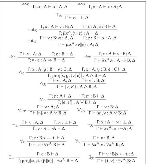
The figures 2.4 and 2.5 summarize the inference rules of respectively classical and intuitionistic first-order minimal sequent calculus, which will be referred to as, respectively, lkm and ljm. The weakening and contraction rules are identical to their non-minimal counterparts.
axL Γ ; α : A⊢ α : A, ∆ axR Γ, x : A⊢ x : A; ∆ ⊤R Γ ⊢ ⋉ : ⊤; ∆ Γ, x : A⊢ v : B; ∆ Γ, x : A; e : B⊢ ∆ cutL Γ ; ˜µxA.hvkei : A ⊢ ∆ Γ ⊢ v : B; α : A, ∆ Γ ; e : B⊢ α : A, ∆ cutR Γ ⊢ µαA.hvkei : A; ∆ Γ ⊢ v : A; ∆ Γ ; e : B⊢ ∆ ⇒L Γ ; v· e : A ⇒ B ⊢ ∆ Γ, x : A⊢ v : B; ∆ ⇒R Γ ⊢ λxA.v : A⇒ B; ∆ Γ, x : A, y : B⊢ v : C; ∆ Γ, x : A, y : B; e : C⊢ ∆ ∧L Γ ; proj[x, y,hvkei] : A ∧ B ⊢ ∆ Γ ⊢ v : A; ∆ Γ ⊢ v′: B; ∆ ∧R Γ ⊢ (v, v′) : A ∧ B; ∆ Γ ; e : A⊢ ∆ Γ ; e′: B⊢ ∆ ∨L Γ ; [e, e′] : A ∨ B⊢ ∆ Γ ⊢ v : A; ∆ ∨1R Γ ⊢ injlv : A ∨ B; ∆ Γ ⊢ v : B; ∆ ∨2R Γ ⊢ injrv : A ∨ B; ∆ Γ ⊢ v : A; ∆ Γ, ⋊ :⊥ ⊢ ∆ ¬L Γ ; v· ⋊ : ¬A ⊢ ∆ Γ ; x : A⊢ ⋊ : ⊥, ∆ ¬R Γ ⊢ λxA.⋊ : ¬A; ∆ Γ ; e : B[x← t] ⊢ ∆ ∀L Γ ; t· e : ∀xA.B⊢ ∆ Γ ⊢ v : B; ∆ ∀R Γ ⊢ λxA.v :∀xA.B; ∆ Γ ; e : B⊢ ∆ ∃L Γ ; proj[α, β,hβkei] : ∃αA.B⊢ ∆ Γ ⊢ v : B[x ← t]; ∆ ∃R Γ ⊢ (t, v) : ∃xA.B; ∆