Identification de dynamique pour les systèmes bilinéaires et non-linéaires en présence d'incertitudes

(1)

THÈSE DE DOCTORAT

de

l’Université de recherche Paris Sciences et Lettres

PSL Research University

Préparée à

l’Université Paris-Dauphine

COMPOSITION DU JURY :

Soutenue le

par

École Doctorale de Dauphine — ED 543 Spécialité

Dirigée par

Identification de dynamique pour des systèmes bilinéaires

et non-linéaires en présence d'incertitudes

09/12/2016

FU Ying

TURINICI Gabriel INRIA Paris-Rocquencourt M. MAZYAR Mirrahimi Université de Bourgogne M. SUGNY Dominique M. LE BRIS Claude

Ecole Nationale de Ponts et Chaussées

M. SALOMON Julien Université Paris Dauphine

M. TURINICI Gabriel Université Paris Dauphine Sciences Rapporteur Rapporteur Président du jury Membre du jury Directeur de thèse

(2)

(3)

Thèse effectuée au sein du Laboratoire CEREMADE de l’Université Paris-Dauphine

Place du Maréchal de Lattre de Tassigny 75016 Paris

(4)

(5)

RÉSUMÉ iii

Résumé

Dans le cadre du contrôle quantique bilinéaire, cette thèse étudie la pos-sibilité de retrouver l’Hamiltonien et/ou le moment dipolaire à l’aide

de mesures d’observables pour un ensemble grand de contrôles. Si

l’implémentation du contrôle fait intervenir des bruits alors les mesures prennent la forme de distributions de probabilité. Nous montrons qu’il y a toujours unicité (à des phases près) des Hamiltoniens de du moment dipolaire retrouvés. Plusieurs modèles de bruit sont étudiés: bruit dis-crète constant additif et multiplicatif ainsi qu’un modèle de bruit dans les phases sous forme de processus Gaussien. Les résultats théoriques sont illustrés par des implémentations numériques.

Mots-clé:

équation Schrödinger, système bilinéaire, contrôle quantique, identifica-tion Hamiltonien

(6)

(7)

Dynamic identification for bi-linear

and non-linear systems in presence of

(8)

(9)

ABSTRACT v

Abstract

The problem of recovering the Hamiltonian and dipole moment, termed inversion, is considered in a bilinear quantum control framework. The process uses as inputs some measurable quantities (observables) for each admissible control. If the implementation of the control is noisy the data available is only in the form of probability laws of the measured observ-able. Nevertheless it is proved that the inversion process still has unique solutions (up to phase factors). Several models of noise are considered including the discrete noise model, the multiplicative amplitude noise model and a Gaussian process phase model. Both theoretical and nu-merical results are established.

Keywords:

Schrödinger equation, bi-linear system, quantum control, inversion Hamil-tonian

(10)

(11)

REMERCIEMENTS vii

Acknowledgements

This thesis is written based on a 3 years professional work, with the kind help and advises of a number of individuals.

First of all, let me extend my thanks to M. MAZYAR Mirrahimi and M. SUGNY Dominique, for writing a report to this work. I am also grateful to M. LE BRIS Claude and M. SALOMON Julien for their participa-tions as members of examination committee.

My most sincere gratitude is to my advisor M. TURINICI Gabriel for his expertise, understanding, patient and generous guidance, encourage-ment and support. I am very glad to finish several works and this thesis with him.

I am grateful to Université Paris Dauphine and the laboratory CERE-MADE for the financial support of this thesis. Thanks for giving me the chance to participate in several meetings and congress. I would also like to thank the members of CEREMADE for the weekly seminars and frequent discussions.

Special thanks to the project EMAQS and all the participants of this project for exchanging the newest results and technologies in quantum control theories. I am also highly indebted to M. Rabitz Herschel and his research group for sharing their knowledge in physics.

Last but not the least, thanks to my parents and my friends for their support.

(12)

(13)

Introduction

In this thesis, the bi-linear system we study is the Schrödinger equa-tion. Quantum system inversion concerns learning the characteristics of the underlying Hamiltonian by measuring suitable observables from the responses of the system’s interaction with members of a set of applied fields. Various aspects of inversion have been confirmed in theoretical, numerical and experimental works. The theoretical part of the thesis addresses the uniqueness, and the numerical part consists in the inver-sion and recovery problem. Various noise models are considered. The plan of the thesis is the following.

The first chapter of the thesis introduces the mathematical formulation of the problem. We start with some examples of applications of quantum mechanics. Then we introduce the basic elements of quantum theory: the state vectors, the observables, and the density operators. Once these notations are defined, we can write the Schrödinger equation. We con-tinue by giving the noise model appearing in the interaction between the electromagnetic field and a quantum system. We go on with a brief introduction of the Lie group and Lie algebra, which are essential in the study of controllability of the Schrödinger equation. The last part of this chapter concerns the distances between the probability distributions and Gaussian process theory which is crucial in numerical simulations. The second chapter reproduces the content of the accepted paper [18]. In this section, the noise is modeled as a discrete random variable. We

(18)

2 INTRODUCTION

first improve the hypotheses of uniqueness result in [29]. Then we prove that in presence of a discrete noise, the Hamiltonian H and the dipole moment µ of the system are unique within some phases. Numerical sim-ulations in the case of additive noise shows that the we can recovery the

H and µ from experimental data.

The third chapter reproduces the content of the accepted paper [19]. In this chapter, we consider the amplitude noise model. The noise is sup-posed to be multiplicative and identical for all frequencies. In contrast to the previous chapter, the noise is supposed to be unknown. Theo-retical results and numerical simulations show that not only the dipole moment but also the noise distribution are unique within some factors and phases and can be recovered.

The fourth chapter discuss the phase noise model. The noises related to different frequencies are correlated and are modeled by Gaussian process in the frequency space. Numerical tests are implemented for the square exponential covariance model, the Ornstein-Uhlenbeck process and the Brownian motion.

(19)

Résumé de la thèse

Ce chapitre est un résumé en français de cette thèse. Le plan et les principaux résultats de cette thèse sont présentés dans ce ré-sumé. Chapitre 1 introduit les ingrédients pour la formulation mathématique du problème étudié. Chapitre 2, 3 et 4 présen-tent les résultats théoriques et numériques avec les modèles de bruit dans les trois cas: variable aléatoire discrète, multiplica-tive de loi inconnue sur les amplitudes et processus Gaussian sur les phases respectivement.

(20)

4 RÉSUMÉ

Nous présentons par la suite les principaux résultats de cette thèse.

0.1 Chapitre 1: formulation mathématique du

prob-lème

Le chapitre 1 consiste en une introduction aux formulations mathéma-tiques des problèmes étudiés dans cette thèse. On commence par donner des exemples d’applications en mécanique quantique. Ensuite on intro-duit les ingrédients essentiels de la mécanique quantique: les états, les observables et les matrices de densité. On continue avec l’équation de Schrödinger et modélisations du bruit apparaissant lors de l’intéraction entre un champ électromagnétique et un système quantique. La présen-tation se poursuit avec une brève introduction aux algèbres et groupes de Lie qui seront invoqués lors de l’étude des résultats de contrôlabilité de l’équation de Schrödinger. A la fin on donne quelques outils concer-nant les distances entre des lois de probabilité, ainsi que des rudiments de la théorie des processus gaussiens, qui seront nécessaires pour la for-mulation de nos sifor-mulations numériques.

(21)

0.2 NOTATIONS 5

0.2 Notations

Les notations suivantes sont utilsées dans les Chapitres 2, 3 et 4:

• LM1,M2,··· ,Mm est l’algèbre de Lie généréé par les matrices M1, M2,· · · , Mm;

• pour tout matrice ou vecteur X, on note par X son conjugué et Xú

la matrice adjointe;

• H est l’ensemble de matrices Hermitiennes. H = _{{X œ C}N◊N_|Xú =

X_};

• _SN est la sphére unitaire de CN : SN = {v œ CN|ÎvÎ = 1};

• Ψ(t, H, u(_{·), µ, Ψ}0) est la solution de la équation (3), pour simplifier

la notation, on la note Ψ(t);

• ⁄k(X), k = 1, ..., N sont les valeurs propres de X œ H dans l’ordre

croissant; on introduit aussi „k(X) les vecteurs propres de X pour

k = 1, ..., N (qui forment une base orthonormée de CN) correspon-dent aux valeurs propres ⁄k(X); le choix n’est pas unique;

• SU (N ) est le group special unitaire de degré N , qui est l’ensemble

de matrices unitaires de tailles N _{◊ N avec determinant 1;}

(22)

6 RÉSUMÉ

0.3 Résultats de contrôlabilité

Dans la suite on introduit quelques résultats de contrôlabilité.

Soit L _{œ N}ú et L groupes de Lie G1,· · · , GL de dimension finie, connexes

et compacts avec élément neutre Id. Soient A¸, B¸ œ g¸ pour tout ¸ =

1,_{· · · , L avec g}¸ L’algèbre de Lie associée à G¸.

Definition 0.1 Soient L systèmes bilinéaires:

Y _ _ _ ] _ _ _ [ dX¸(t) dt = (A¸ + u(t)B¸)X¸(t), X¸ œ G¸ X¸(0) = Id œ G¸. (1)

Les systèmes sont dites simultanément contrôlables s’il existe

TA1,··· ,AL,B1,··· ,BL > 0 tel que pour tout T Ø TA1,··· ,AL,B1,··· ,BL et pour

tout V¸ œ G¸, ¸ = 1,· · · , L arbitairement choisis, il existe un contrôle

u œ L1_{([0, T ], R) avec X}

¸(T ) = V¸, ’¸ = 1, · · · , L.

Soient _{A = A}1m· · ·mAL œ mL¸=1g¸ et B = B1m· · ·mBL œmL¸=1g¸.

Theorem 0.1 La collection (1) de L systèmes bilinéaires est

simultané-ment contrôlable si et seulesimultané-ment si L_A,B = mL

¸=1g¸ (ou dimRL_A,B = qL

¸=1dimRg_¸.

Lemma 0.1 On suppose que LA¸,B¸ = g¸ pour tout ¸ = 1,· · · , L. Alors

L_A,B _”= mL

¸=1g¸ si et seulement si il existent ¸, ¸Õ œ {1, · · · , L}, ¸ ”= ¸Õ

et un isormorphisme f : g¸ æ g¸Õ tels que f (A_¸) = A_¸Õ et f (B_¸) = B_¸Õ.

Theorem 0.2 Soit G un groupe de Lie de dimension finie, connexe,

compact et simple et g l’algèbre de Lie associée. Soient A, B œ g tels

que LA,B = g et –1,...,–L œ R sont les réels, –i ”= –j ’i ”= j. On

(23)

0.3 RÉSULTATS DE CONTRÔLABILITÉ 7 Y _ _ _ ] _ _ _ [ dX¸(t) dt = {A + (u(t) + –¸)B}X¸(t), X¸(0) = Id. (2)

(24)

8 RÉSUMÉ

0.4 Un exemple de système à nombre fini de niveaux

Pour les simulations numériques intervenant dans cette thèse nous allons utiliser l’équation de Schrödinger:

Y _ _ _ ] _ _ _ [ i ˙Ψ(t, H, u(·), µ, Ψ0) = (H + u(t)µ)Ψ(t, H, u(·), µ, Ψ0) Ψ(0, H, u(·), µ, Ψ0) = Ψ0, (3)

Le choix d’opérateurs H et µ suivra l’exemple introduit dans [14]:

Hréel = Q c c c c c c c c c a 0.0833 _{≠0.0038 ≠0.0087 0.0041} ≠0.0038 0.0647 0.0083 0.0038 ≠0.0087 0.0083 0.0036 ≠0.0076 0.0041 0.0038 _{≠0.0076 0.0357} R d d d d d d d d d b , (4) µréel = Q c c c c c c c c c a 0 5 ≠1 0 5 0 6 _≠1.5 ≠1 6 0 7 0 ≠1.5 7 0 R d d d d d d d d d b . (5)

Pour rappel, sur un tel système il est généralement possible de mesurer des observables du type:

ÈOjÍ(t) = ÈΨ(0, H, u(·), µ, Ψ0)|Oj|Ψ(0, H, u(·), µ, Ψ0)Í, (6)

(25)

0.5 FORMULATION D’UN PROBLÈME D’IDENTIFICATION 9

0.5 Formulation d’un problème d’identification

Lorsque dans l’équation (3) nous connaissons H, µ et Ψ0, nous pouvons

calculer les observables _ÈOjÍ(t), Oj œ H, j = 1, · · · . Le but de cette

thèse est la formulation et l’étude de faisabilité théorique et numérique

du problème, dit inverse, suivant: connaissant quelques _ÈOjÍ(t) pour

certains Oj œ H et t Ø 0, trouver les opérateurs µ et/ou H ( et

occas-sionement Ψ0). Le cas sans bruit a été traité dans [29], nous allons ainsi

(26)

10 RÉSUMÉ

0.6 Chapitre 2: contrôle perturbé par une variable

aléa-toire discrète

Dans ce chapitre, le contrôle est supposé perturbé par une variable aléa-toire discrète, notée Y . On suppose que Y est indépendante du temps. Le contrôle est sous la forme de u(t, ‘(_{·), Y ).}

Le problème d’identification se pose dans deux cas:

• Cas (S1): l’Hamiltonien H est connu et on veut identifier le moment dipolaire µ.

• Cas (S2): ni l’Hamiltonien H ni le moment dipolaire µ ne sont connus.

On commence par rappeler la définition d’ensemble complet d’observables qui commutent (ECOC).

Un ensemble d’observables_{O = {O}1, ..., OK} est dit ensemble d’observables

qui commutent (EOC) si [Ok, O¸] = 0, ’k, ¸ œ {1, ..., K}.

Toutes les observables dans un EOC _{O sont co-diagonalisables.}

C’est-à-dire, il existe au moins une base orthonormée Φ = _{„1, ..., „N} de

CN _{telle que tout O} _{œ O est diagonale dans la base Φ. Un EOC est}

dit ensemble complet d’observables qui commutent (ECOC) si la base orthonormée qui diagonalise le EOC est unique à des phases et permu-tation près.

Le lemme suivant donne une propriété importante de ECOC.

Lemme 1 Soit O = {O1, ..., OK} un EOC. Alors O est un ECOC si et

seulement si il existent “1, ..., “K œ R tels que tous les valeurs propres

de qK

(27)

0.6 CHAPITRE 2: CONTRÔLE PERTURBÉ PAR UNE VARIABLE

ALÉATOIRE DISCRÈTE 11

0.6.1 Inversion sans perturbation

Le problème est d’abord traité dans le cas sans perturbation, c’est-à-dire

Y = 0. Nous améliorons ainsi les résultat dans [29].

Théorème 1 (Cas (S1)) Soient H, µ₁, µ2 œ H, H diagonales, Ψ10, Ψ20 œ

SN. Pour a = 1, 2 et ‘ œ L1loc(R+, R), on note Ψa(t, ‘) = Ψ(t, H, ‘(·), µa, Ψa0).

Soit _{O un EOC non trivial. On suppose que N Ø 3 et}

• (H1): LiH,iµ1 = LiH,iµ2 = su(N ).

• (H2): tr(H) = tr(µ1) = tr(µ2) = 0.

• les valeurs propres de H sont de multiplicité 1. Alors il existe T > 0 tel que si

ÈOΨ1(T, ‘), Ψ1(T, ‘)Í = ÈOΨ2(T, ‘), Ψ2(T, ‘)Í (7)

’‘ œ L1([0, T ]; R), _{’O œ O,}

alors il existent des phases (–i)Ni=1 œ RN telles que:

(µ1)jk = ei(–j≠–k)(µ2)jk, ’j, k Æ N. (8)

L’hypothèse (H1) est nécessaire pour la contrôlabilité simultanée. Par contre on peut poser l’hypothèse (H2) sans perte de généralité.

L’Hamiltonian H et le moment dipolaire µ ne sont identifiables qu’aux phases près. Pour contre-exemple, voir Remarque 2.3, page 79.

Quand les valeurs propres de H sont non dégénérées mais _{O est un}

ECOC, c’est un cas particulier du théorème suivant:

Théorème 2 (Cas (S2)) Soient µ1, µ2, H1, H2 œ H, Ψ10, Ψ20 œ SN. Pour

(28)

12 RÉSUMÉ

O = {O1, ..., OK} un ECOC et Φ = {„1, ..., „N} une base orthonormée

qui diagonalise _{O. On suppose que N Ø 3 et que les hypothèses suivants} sont vraies:

(H1’): LiH1,iµ1 = LiH2,iµ2 = su(N );

(H2’): tr(H1) = tr(H2) = tr(µ1) = tr(µ2) = 0;

Alors il existe T > 0 tel que si

ÈOkΨ1(T, ‘), Ψ1(T, ‘)Í = ÈOkΨ2(T, ‘), Ψ2(T, ‘)Í (9)

’‘ œ L1([0, T ]; R), ’k = 1, · · · , K,

alors il existent des phases (–i)Ni=1 œ RN et ◊ œ R telles que pour tout

j, k _{Æ N, soit} Y _ _ _ _ _ _ _ ] _ _ _ _ _ _ _ [ Èµ1„j, „kÍ = ei(–j≠–k)Èµ2„j, „kÍ ÈH1„j, „kÍ = ei(–j≠–k)ÈH2„j, „kÍ ÈΨ10, „jÍ = ei(◊≠–j)ÈΨ20, „jÍ, (10) soit Y _ _ _ _ _ _ _ ] _ _ _ _ _ _ _ [ Èµ1„j, „kÍ = ≠ei(–j≠–k)Èµ2„j, „kÍ ÈH1„j, „kÍ = ≠ei(–j≠–k)ÈH2„j, „kÍ ÈΨ1 0, „jÍ = ei(◊≠–j)ÈΨ20, „jÍ. (11)

Quand _{O n’est pas un ECOC, la preuve permet d’obtenir l’existence}

d’un isomorphisme d’algèbres de Lie qui envoie iH1 en iH2 et iµ1 en

(29)

0.6.2 Inversion en présence de perturbation de loi connue

Soit (Ω,_{F, P) un espace de probabilité discret, V = {y}¸ œ Rd|¸ œ I µ N}

un ensemble inclus dans Rd (qui peut être infini). La perturbation est modélisée par une variable aléatoire discrète Y : Ω _{æ V.}

On peut supposer que pour tout y¸ œ V, P(Y = y¸) > 0 et I = Nú ou

I = {1, · · · , L0} avec L0 œ Nú. On note ›k = P(Y = yk), ’k œ I. On

suppose que (›¸)¸Ø1 est une suite décroissante en permutant les indices.

En particulier la loi de Y est complètement donnée par la connaissance de _{V et des (›}¸)¸Ø1 qui sont supposées connues.

Un lemme essentiel pour la démonstration du résultat d’identification dans ce cas est le suivant:

Lemme 2 Soit Ja : CN◊N æ R, a = 1, 2 et h : Rd+1 æ R des fonctions

analytiques réelles avec Ja bornée. Soit Aa, Ba œ su(N), T > 0, ‘ œ

L1([0, T ], R) et on note Xa(t, y¸, ‘) la solution de Y _ _ _ ] _ _ _ [ dXa(t,y¸,‘) dt = (Aa+ h(‘(t), y¸)Ba)Xa(t, y¸, ‘) Xa(0, y¸, ‘) = Id, (12) pour a = 1, 2 et tout ¸ _{œ I.}

On suppose avoir l’égalité en loi suivante:

LY(J1(X1(T, Y, ‘))) = LY(J2(X2(T, Y, ‘))) ’‘ œ L1([0, T ], R). (13)

Alors pour tout ¸ _{œ I, il existent n}0(¸, ›1,· · · , ›n,· · · ) et un indice Ÿ(¸) œ

I, Ÿ(¸) Æ n0(¸, ›1,· · · , ›n,· · · ) tels que

(30)

14 RÉSUMÉ

Dans la suite, on suppose que la perturbation est additive. C’est-à-dire

u(t) = ‘(t) + Y .

Les résultats principaux de ce chapitre sont les théorèmes suivants: Théorème 3 On considère la même situation et on suppose les mêmes

hypothèses que dans le théorème 2 sauf la relation (9). Alors il existe

T > 0 tel que si:

LYÈOkΨ1(T, ‘ + Y ), Ψ1(T, ‘ + Y )Í = LYÈOkΨ2(T, ‘ + Y ), Ψ2(T, ‘ + Y )Í

(15) ’‘ œ L1([0, T ]; R), _{’k = 1, · · · , K,}

alors les conclusions (10) et (11) du théorème 2 restent vraies.

Ici, le temps T doit être assez grand. La preuve est adaptée pour tout temps Tú supérieur au temps Tú.

De même, pour le cas (S1), on a:

Corollaire 1 On considère la même situation et on suppose les mêmes

T > 0 tel que si:

LYÈOΨ1(T, ‘ + Y ), Ψ1(T, ‘ + Y )Í = LYÈOΨ2(T, ‘ + Y ), Ψ2(T, ‘ + Y )Í

(16)

’‘ œ L1([0, T ]; R), ’O œ O,

alors la conclusion (8) du théorème 1 reste vraie.

Maintenant on suppose que la perturbation est multiplicative. Le

con-trôle est sous la forme de u(t) = Y _{· ‘(t). On suppose en plus que la}

(31)

Corollaire 2 On considère la même situation et on suppose les mêmes

T > 0 tel que si:

LYÈOkΨ1(T, ‘Y ), Ψ1(T, ‘Y )Í = LYÈOkΨ2(T, ‘Y ), Ψ2(T, ‘Y )Í (17)

’‘ œ L1([0, T ]; R), ’k = 1, · · · , K,

alors les conclusions (10) et (11) du théorème 2 restent vraies.

0.6.3 Application numérique: perturbation additive

La simulation numérique est faite dans le cas (C2) pour le système défini par les matrices (4) et (5) (voir section 0.4).

On diagonalise la matrice Hréel avec Hréel = ePréelDe≠Préel,

D = Q c c c c c c c c c a 0 0 0 0 0 0.0365 0 0 0 0 0.0651 0 0 0 0 0.0857 R d d d d d d d d d b ,Preal = Q c c c c c c c c c a 0 1 ≠1 1 ≠1 0 1 1 1 ≠1 0 ≠1 ≠1 ≠1 1 0 R d d d d d d d d d b .

En réalité les valeurs propres de l’Hamiltonien sont connues avec grande précisions. Donc on peut supposer que la matrice D est connue. Alors l’identification de Hréel revient à l’identification de la matrice de

rota-tion antihermitienne _Préel.

(32)

16 RÉSUMÉ

utilise plusieurs contrôles sous la forme

‘(t) = exp Q c a≠40 Q a t_{≠ T/2} T R b 2R d b ÿ 1_Æi<jÆN

Aijsin[(⁄j(Hréel)≠⁄i(Hréel))t+◊ij].

(18) Ici ⁄i(Hréel) sont les valeurs propres de Hréel, i Æ N et Aij, ◊ij des

paramètres de notre choix. Le temps total de simulation est T = 3200 qui correspond à 10 périodes de la plus petite transition ⁄4(Hreal) ≠

⁄3(Hreal).

Les observables choisies sont les populations _{O = {e}keúk, k Æ N}

asso-ciées à la base canonique _{ek; k Æ N}. On choisit N‘ = 36 contrôles

‘1(t), ..., ‘N‘(t) avec ◊ij arbitairement dans [0, 2ﬁ] et Aij arbitairement

dans [0, 0.0012] et la fonction à minimiser est:

J (P, µ) = N‘ ÿ i=1 N ÿ j=1 d_W1(LY(|ÈΨ(T, ePDe≠P, ‘i + Y, µ, Ψ 0 1), ejÍ|2,

LY(|ÈΨ(T, Hréel, ‘i + Y, µreal, Ψ0réel), ejÍ|2). (19)

La distance qu’on utilise ici est la 1-distance de Wasserstein.

On commence par une erreur relative de 10% sur µ et _{P. Après 277}

itérations, on obtient: P277 = Q c c c c c c c c c a 0 0.999 _{≠0.999 1.002} ≠0.999 0 1 0.999 0.999 ≠1 0 ≠1.002 ≠1.002 ≠0.999 1.002 0 R d d d d d d d d d b ,

(33)

0.6 CHAPITRE 2: CONTRÔLE PERTURBÉ PAR UNE VARIABLE ALÉATOIRE DISCRÈTE 17 µ277 = Q c c c c c c c c c a 0 4.999 _{≠0.998 ≠0.003} 4.999 0 6 ≠1.5 ≠0.998 6 0 7 ≠0.003 ≠1.5 7 0 R d d d d d d d d d b .

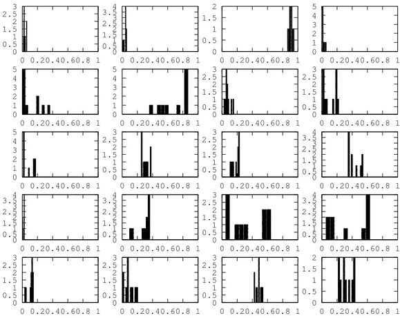
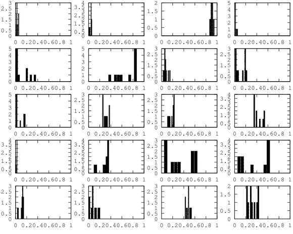
Ces résultats correspondent aux erreurs relatives de 0.003% sur µ et 0.001% sur_{P. Les figures Figure} 1et Figure2montrent que l’algorithme converge bien vers le système réel.

0 0.5 1 1.5 2 2.5 3 0 0.20.40.60.8 1 0 0.51 1.5 2 2.53 3.54 0 0.20.40.60.8 1 0 0.5 1 1.5 2 0 0.20.40.60.8 1 0 1 2 3 4 5 0 0.20.40.60.8 1 0 1 2 3 4 5 0 0.20.40.60.8 1 0 1 2 3 4 5 0 0.20.40.60.8 1 0 0.5 1 1.5 2 2.5 3 0 0.20.40.60.8 1 0 0.5 1 1.5 2 2.5 3 0 0.20.40.60.8 1 0 1 2 3 4 5 0 0.20.40.60.8 1 0 0.5 1 1.5 2 2.5 3 0 0.20.40.60.8 1 0 0.5 1 1.5 2 2.5 3 0 0.20.40.60.8 1 0 0.5 1 1.52 2.53 3.5 4 0 0.20.40.60.8 1 0 0.51 1.52 2.53 3.54 0 0.20.40.60.8 1 0 0.51 1.52 2.53 3.54 0 0.20.40.60.8 1 0 0.5 1 1.5 2 2.5 3 0 0.20.40.60.8 1 0 0.51 1.52 2.53 3.54 0 0.20.40.60.8 1 0 0.5 1 1.5 2 2.5 3 0 0.20.40.60.8 1 0 0.5 1 1.5 2 2.5 3 0 0.20.40.60.8 1 0 0.5 1 1.5 2 2.5 3 0 0.20.40.60.8 1 0 0.5 1 1.5 2 0 0.20.40.60.8 1

Figure 1: On figure l’histogramme des lois _LY(|ÈΨ(T, ePrealDe≠Preal, ‘i +

(34)

18 RÉSUMÉ 0 0.5 1 1.5 2 2.5 3 0 0.20.40.60.8 1 0 0.51 1.52 2.5 3 3.54 0 0.20.40.60.8 1 0 0.5 1 1.5 2 0 0.20.40.60.8 1 0 1 2 3 4 5 0 0.20.40.60.8 1 0 1 2 3 4 5 0 0.20.40.60.8 1 0 1 2 3 4 5 0 0.20.40.60.8 1 0 0.5 1 1.5 2 2.5 3 0 0.20.40.60.8 1 0 0.5 1 1.5 2 2.5 3 0 0.20.40.60.8 1 0 1 2 3 4 5 0 0.20.40.60.8 1 0 0.5 1 1.5 2 2.5 3 0 0.20.40.60.8 1 0 0.5 1 1.5 2 2.5 3 0 0.20.40.60.8 1 0 0.51 1.5 2 2.53 3.54 0 0.20.40.60.8 1 0 0.51 1.5 2 2.53 3.54 0 0.20.40.60.8 1 0 0.51 1.5 2 2.53 3.54 0 0.20.40.60.8 1 0 0.5 1 1.5 2 2.5 3 0 0.20.40.60.8 1 0 0.51 1.5 2 2.53 3.54 0 0.20.40.60.8 1 0 0.5 1 1.5 2 2.5 3 0 0.20.40.60.8 1 0 0.5 1 1.5 2 2.5 3 0 0.20.40.60.8 1 0 0.5 1 1.5 2 2.5 3 0 0.20.40.60.8 1 0 0.5 1 1.5 2 0 0.20.40.60.8 1

Figure 2: On figure l’histogramme des lois LY(|ÈΨ(T, eP277De≠P277, ‘i +

(35)

0.7 CHAPITRE 3: PERTURBATION MULTIPLICATIVE DE LOI

INCONNUE SUR LES AMPLITUDES 19

0.7 Chapitre 3: perturbation multiplicative de loi

in-connue sur les amplitudes

Dans ce chapitre, les perturbations sont dans les amplitudes. On sait que dans le laboratoire, le contrôle est une superposition de plusieurs fréquences:

u(t) = ‡(t) ÿ

–”=—

A–—sin(Ê–—t + ◊–—), (20)

avec ‡(t) est une fonction Gaussian en temps et Ê–— = E— ≠ E– les

transitions liées aux valeurs propres de H E– et E— . Les amplitudes

A–— et les phases ◊–— sont des paramètres à contrôler.

En réalité, quand on rèpète la même expérience plusieurs fois, il y aura des perturbations dans les amplitudes. C’est-à-dire pour chaque expéri-ence, il y a un facteur multiplicatif sur le contrôle. La perturbation est modélisée par une variable aléatoire Y , le contrôle est sous la forme

multiplicative Y _{· u(t). On fait l’hypothèse que les perturbations sur}

toutes les amplitudes sont identiques. En plus on ne considère pas de perturbations sur les phases ◊–—.

Le support de la perturbation Y est un ensemble fini _{V = {y}¸, ¸Æ L} µ

R_{. Ainsi la distribution de Y est complètement définie par les} probabil-ités ›¸ = P(Y = y¸).

A la différence du chapitre précédant, la distribution (›¸)L¸=1 fait partie

des inconnues du problème. L’ensemble _{V est supposé donné (ce qui}

n’enlève en pratique rien à la généralité du problème, car on peut pren-dre _{V aussi grand que nécessaire).}

(36)

20 RÉSUMÉ

Le théorème suivant montre que sous certaines hypothèses, si on obtient

les même distributions pour tous les observables dans un EOC _{O et tous}

les contrôles, alors le moment dipolaire µ et les probabilités (›¸)L¸=1 sont

identifiables à des phases multiplicatives près.

Théorème 4 Soient H, µ1, µ2 œ H, H diagonale, µ1 ”= 0, µ2 ”= 0, Y1, Y2

deux variables aléatoires avec le même support _{V qui contient au moins} un élement non nul, Ψ1₀, Ψ2₀ _{œ S}N des états initiaux et pour a = 1, 2 et

u _{œ L}1_loc(R+, R), on note: Ψa(t, u) = Ψ(t, H, u(·), µa, Ψa0). Soit O un

EOC non trivial.

On suppose que N _{Ø 3 et les hypothèses suivants:} 1. LiH,iµ1 = LiH,iµ2 = su(N );

2. tr(H) = tr(µ1) = tr(µ2) = 0;

3. les valeurs propres de H sont tous de multiplicité 1. 4. _|(µ1)k,¸|2 = |(µ2)k,¸|2 ”= 0 pour un couple (k, ¸) fixé. .

Le temps final d’observation est noté T et est supposé assez grand. Si on a l’égalité de distributions suivante:

L(ÈOΨ1(T, uY1), Ψ1(T, uY1)Í) = L(ÈOΨ2(T, uY2), Ψ2(T, uY2)Í) (21)

’u œ L1([0, T ]; R), _{’O œ O,}

alors il existent des phases (–i)N_i=1 œ RN telles que

Y _ _ _ ] _ _ _ [ (µ1)jk = ±ei(–j≠–k)(µ2)jk, ’j, k Æ N, P_(Y₁ _{= y}_¸_{) = P(Y}₂ ₌ _±y_¸₎ _{’¸ Æ L.} (22) On remarque que si le couple (Y, µ) est une solution, alors toutes les couples (Y /⁄, ⁄µ) sont des solutions.

(37)

Plusieurs simulations numériques sont faites avec le système défini par les matrices (4) et (5).

On suppose que l’Hamiltonien H est connu, donc les observables _{O =}

{O1, ..., OK} sont les projections {|e1ÍÈe1|, ... , |eNÍÈeN|} sur une base

propre de H. Ici _|e1Í est le je vecteur propre de H.

Les expériences sont répétés pour plusieurs contrôles u1,...,uNu et on

minimise le critère défini par

J (µ, (›k)Lk=1; (ui)Ni=1u ) = log Y ] [ 1 Nu Nu ÿ i=1 N ÿ j=1W 1 S U L ÿ k=1 ›_k”_|ÈΨ(T,H,u_i_·y_k_,µ,Ψ0 1),ejÍ|2, L ÿ k=1

›_kreal”_|ÈΨ(T,H,u_i_·y_k_,µ_real_,Ψ0 1),ejÍ|2 T V Z ^ \ . (23)

On commence par un choix initial µ0 et une distribution initiale ›0 qui est la loi uniforme. L’itération n _{Ø 1 consiste en plusieurs étapes:}

1. On choisit arbitairement Nu contrôles uni, i = 1, ..., Nu ;

2. on minimise › _{æ J (µ}n≠1, ›; (ui)Ni=1u) et on note par ›n le minimiseur;

3. on minimise µ _{æ J (µ, ›}n; (ui)Ni=1u ) and on note par µn un

min-imiseur.

Pour les illustrations numériques on prend Nu = 36; les amplitudes

(A–—) sont uniformément prises dans [0, 0.0012] et les phases ◊–— dans

[0, 2ﬁ].

(38)

22 RÉSUMÉ µ0_g = Q c c c c c c c a 0 3.76 _≠1.31 0 3.76 0 3.51 _≠1.78 ≠1.31 3.51 0 6.72 0 _{≠1.78 6.72} 0 R d d d d d d d b , (24) µ0_e = Q c c c c c c c a 0 10 1 1 10 0 10 1 1 10 0 10 1 1 10 0 R d d d d d d d b , (25) µ0_b = Q c c c c c c c a 0 7.48 _≠0.51 0 7.48 0 8.83 _≠0.87 ≠0.51 8.83 0 5.87 0 _{≠0.87 5.87} 0 R d d d d d d d b . (26)

Les observables sont des projections _{|e1ÍÈe1|, |e2ÍÈe2|, |e3ÍÈe3|, |e4ÍÈe4|}

sur les vecteurs propres:

|e1Í = 1 0.0845 _{≠0.1313 0.9651 0.2101}2T, |e2Í = 1 ≠0.1305 ≠0.0856 ≠0.2103 0.96512T , |e3Í = 1 0.2118 0.9647 0.0838 0.13252T , |e4Í = 1 0.9649 _{≠0.2118 ≠0.1314 0.0830}2T . (27)

On pose le temps final T = 3200 et on suppose que _|(µreal)12|2 = 25 est

connu.

Le support de la distribution Y est connu et on le note [ym, yM]. On

prend ym = 0.5 et yM = 1.5. On discrétise le support avec L = 51 points

equidistants y¸ = ym+(¸≠1)·yM_L≠y_≠1m, ¸ = 1, ..., L. Plusieurs distributions

(39)

• Yreal = Yg la distribution Gaussienne centrée en 1 avec la variance 0.0025 (voir équation (3.17) dans section 3.3.2);

• Yreal = Ye la distribution exponentielle déplacée (voir équation

(3.18) dans section 3.3.2);

• Yreal = Yb la distribution bi-modale qui est la somme des deux

distributions Gaussiennes: la première est centrée en 0.8 avec la variance 0.0025 et la seconde est centrée en 1.2 avec la variance 0.0049 (voir équation (3.19) dans section 3.3.2).

Après 10 itérations, on obtient:

Îµ10g ≠ µrealÎ_Œ = 5· 10≠5, µ10g = Q c c c c c c c c c a 0 5 _≠1 0 5 0 5.99995 ≠1.5 ≠1 5.99995 0 6.99999 0 _≠1.5 6.99999 0 R d d d d d d d d d b , (28) Îµ10e ≠ µrealÎŒ = 10≠4, µ10e = Q c c c c c c c c c a 0 5 ≠1 0 5 0 6 ≠1.5 ≠1 6 0 6.9999 0 ≠1.5 6.9999 0 R d d d d d d d d d b , (29) Îµ10b ≠ µrealÎŒ = 6· 10≠5, µ10b = Q c c c c c c c c c a 0 5 ≠1 0 5 0 5.99999 ≠1.5 ≠1 5.99999 0 6.99994 0 ≠1.5 6.99994 0 R d d d d d d d d d b . (30)

(40)

24 RÉSUMÉ

Les figures 3.1,3.2, 3.3 et les tableaux 3.1 et 3.2 présentent la conver-gence de l’algorithme.

La simulation est aussi faite dans le cas où on utilise juste une observable qui est la projection _|e3ÍÈe3|. Le choix initial est

µ0_b = Q c c c c c c c a 0 10 1 1 10 0 10 1 1 10 0 10 1 1 10 0 R d d d d d d d b , (31)

La distribution Yreal testée est la distribution bimodale. Après 5,10 et 15 itérations, le moment dipolaire obtenu ont respectivement les erreurs

L2 de 0.17246, 0.03736 et 4.5652_{· 10}≠4. La vitesse de convergence est moins rapide que dans le cas précédent.

(41)

0.8 CHAPITRE 4: PERTURBATION SUR LES PHASES 25

0.8 Chapitre 4: perturbation sur les phases

Dans ce chapitre nous considérons un modèle de bruit de loi paramétrique (avec paramètre connu). Le bruit est cette fois-ci une fonction dépen-dante de la fréquence (en particulier donc pas constant).

On commence par écrire le contrôle comme une intégrale sur les fréquences:

u(t) = S(t)⁄

ÊœDA(Ê)cos(Êt + ◊(Ê))dÊ. (32)

Ici_{D est une partie bornée de R}+qui répresente l’ensemble des fréquences

possibles. S(t) est une enveloppe Gaussienne dans le temps. Les

am-plitudes A(Ê) : _{D æ R}+ et les phases ◊(Ê) : D æ [0, 2ﬁ] sont les

paramètres nominaux du contrôle. Les amplitudes A doivent être inté-grable sur _D.

Dans ce chapitre, on considère des perturbations dans les phases qui sont modélisées comme un processus Gaussien indexé par les frequences. On introduit le modèle suivant:

u(t) = S(t)⁄

Ê_œDA(Ê)cos(Êt + ◊(Ê) + ”◊Ê). (33)

Les perturbations dans les phases sont (”◊Ê)ÊœD.

En pratique, les physiciens utilisent un nombre fini de frequences pour construire le contrôle. Notons par NÊ ce nombre. Alors une

discrétisa-tion de l’équadiscrétisa-tion (33) est:

u(t) = S(t)

NÊ

ÿ

l=0

Alcos(Êlt + ◊l + ”◊l), (34)

(42)

26 RÉSUMÉ

L’espérance de u(t) est E(u(t)) = –u0(t) avec u0(t) = S(t)qN_l=1Ê Alcos(Êlt+

◊_l) le contrôle sans perturbation et – =qŒ

k=0(≠1)k (2k)!2k_k!‡2k.

Les observables qu’on utilise dans ce chapitre sont les projections sur une base propre de H: _{O = {O}1, ..., ON} = {|e1ÍÈe1|, ... , |eNÍÈeN|}

avec _|eiÍ le ie vecteur propre de H.

Les fréquences (Êl)1ÆlÆNÊ sont choisies comme les transitions des valeurs

propres de H: _|⁄i ≠ ⁄j|, avec (⁄i)1ÆiÆN les valeurs propres de H. En

particulier, NÊ = N (N₂≠1).

Le processus Gaussien (”◊Ê)ÊœD est simulé par Nr réalisations aléatoires.

La distribution du contrôle simulé u(t) est donc

Lu(t) = Nr ÿ k=1 1 Nr ”_S(t)qNÊ l=1Alcos(Êlt+◊l+”◊l,k), (35) où (”◊l,k)1ÆlÆNÊ,1ÆkÆNr œ R NÊ·Nr sont N r réalisations.

On minimise un critère construit avec des contrôles (uj₎

1ÆjÆNu et (˜u

j₎

1ÆjÆNu

defini par Nucouples d’amplitudes différentes (Ajl)1ÆjÆNu,1ÆlÆNÊ et phases

différentes (◊_lj)_1ÆjÆNu,1ÆlÆNÊ.

Chaque uj est simulé avec Nr réalisations (”◊l,kj )1ÆlÆNÊ,1ÆkÆNr œ R

NÊ·Nr: Luj_(t) = Nr ÿ k=1 1 Nr ”_S(t)qNÊ l=1A j lcos(Êlt+◊jl+”◊ j l,k). (36)

(43)

0.8 CHAPITRE 4: PERTURBATION SUR LES PHASES 27 ˜ uj(t) = S(t) NÊ ÿ l=0 Aj_lcos(Êlt+ ◊lj + ”◊l). (37)

La critère à minimiser est:

J (uj, µ, ˜uj, µreal) = N ÿ i=1W1 (|ÈΨ(T, H, uj, µ, Ψ0), eiÍ|2, |ÈΨ(T, H, ˜uj, µreal, Ψ0), eiÍ|2), (38) Sa moyenne est: ˜ J ((uj)1_ÆjÆNu, µ, (˜u j₎ 1_ÆjÆNu, µreal) = 1 Nu Nu ÿ j=1J (u j_{, µ, ˜}_uj_{, µ} real). (39)

Plusieurs simulations numériques sont faites avec le système défini par les matrices (4) et (5).

On choisit Nu = 36. Les amplitudes sont prises uniformément dans

[0, 0.0012] et les phases dans [0, 2ﬁ]. On commence par

µ0 = Q c c c c c c c c c a 0 5.1295 ≠0.9762 0.0962 5.1295 0 5.5100 _≠1.6434 ≠0.9762 5.5100 0 7.6117 0.0962 _{≠1.6434 7.6117} 0 R d d d d d d d d d b , (40)

qui correspond à une erreur relative de 8.7%.

On choisit la covariance de double exponentiel (voir exemple 1.3) pour les perturbations:

(44)

28 RÉSUMÉ

Σl,lÕ = ‡2e≠

(Êl≠ÊlÕ)2

— (41)

avec — un paramètre réel. On pose ‡ = 0.1.

La valeur — doit être bien calibrée pour que les perturbations soient corrélées mais pas trop corrélées. Les figures Figure 4.1, Figure 4.2 et

Figure 4.3 montrent que — = 0.1 est un bon choix.

On pose Nr = 1000. Après 50 itérations, on obtient:

µ50 = Q c c c c c c c c c a 0 4.9781 _{≠0.9307 ≠0.0063} 4.9781 0 5.9568 _≠1.5189 ≠0.9307 5.9568 0 7.0682 ≠0.0063 ≠1.5189 7.0682 0 R d d d d d d d d d b ,

qui correspond à une erreur relative de 1%.

Maintenant on utilise le modèle de matrice de covariance exponentielle (voir exemple 1.4):

Σl,lÕ = ‡2e≠ |Êl≠ÊlÕ|

—Õ . (42)

Un bon candidat de —Õ est —Õ = 2 (voir Figure 4.8). Cette fois Nr = 100.

Après 60 itérations, on obtient

µ60 = Q c c c c c c c c c a 0 5.0641 ≠1.0585 0.0068 5.0641 0 5.9642 _≠1.5139 ≠1.0585 5.9642 0 7.0294 0.0068 ≠1.5139 7.0294 0 R d d d d d d d d d b ,

(45)

0.8 CHAPITRE 4: PERTURBATION SUR LES PHASES 29

qui corresponds à une erreur relative de 0.91%.

Finalement on suppose que la perturbation est un mouvement Brownien dans l’espace des fréquences avec

Σl,lÕ = ‡2min(Ê_l, Ê_lÕ). (43)

On choisit Nr = 100. Après 60 itérations, on obtient

µ60 = Q c c c c c c c c c a 0 5.0043 ≠1.0138 0 5.0043 0 6.0078 _≠1.5015 ≠1.0138 6.0078 0 6.9834 0 ≠1.5015 6.9834 0 R d d d d d d d d d b ,

(46)

(47)

Chapter 1 Mathematical formulation of quantum

mechanics

The quantum theory is widely used in various domains, in-cluding the laser and NMR technology. To give a mathematical formulation of the quantum theory, we introduce the notions of states, observables and density matrices. The main equation we consider in this thesis is the Schrödinger equation. To study the controllability of a Schrödinger equation, the theory of Lie group and Lie algebra is necessary. Some tools concerning the distance between the probability distributions and several basic elements in the Gaussian process theory which are useful in the numerical simulation are also introduced.

(48)

32 CHAPTER 1: MATHEMATICAL FORMULATION OF QUANTUMMECHANICS

1.1 Physical backgrounds

Today, classical physics is still used in much of modern science and tech-nology. However classical physics can only explains energy and matter on a scale familiar to human experience. In the end of 19th century sci-entists discovered phenomena in both macro (the large) and micro (the small) worlds that classical physics could not explain. These limitations led to the development of quantum mechanics.

In contrast to the classical physics, quantum theory is invoked to de-scribe all phenomena from the very small to the very large, covering about sixty orders of magnitude in dimensions. Between these extremes, we find all the objects of the world around us.

In the following, we give some examples of the applications of quantum theory. We cite the presentation in [23] and [33].

1.1.1 Applications of quantum mechanics

Quantum theory as a unifying description of Nature As a proof of

the success of quantum theory stands, the unification of three out of the four fundamental interactions – the electromagnetic, strong and weak forces – in the Standard Model, which reveals the deep symmetries of Nature. These are also the promising attempts to include gravitation in a unified theory of strings. And all physicists will certainly emphasize the universality of physics, a remarkable consequence of quantum laws. It is the quantum theory which explains the radiation spectrum of hydro-gen in our laboratory lamps, but also in intergalactic space. Quantum chemistry applies to the reactions in laboratory test tubes, but also to the processes in the interstellar dust where molecules are formed and destroyed, producing radiation detected by our telescopes after traveling billions of years through space. Let us finally evoke cosmology and the remarkable link between the infinitely small and large scales, underlined

(49)

1.1 PHYSICAL BACKGROUNDS 33

by the quantum theory. It emphasizes the similarity between the phe-nomena which occurred at the origin of the Universe, in a medium of inconceivably large temperature and density, and those which happen in the violent collisions between particles studied by large accelerators on Earth.

The laser and the optical revolution The laser is an example of

an-other invention based on a quantum idea. Light had been forever made of random waves, difficult to direct, to focus or to force to oscillate at a well-defined frequency. The laser has changed this state of affairs and has allowed us to tame radiation by exploiting the properties of atomic stimulated emission, discovered by Einstein at the dawn of the quantum era. Lasers now have a huge variety of uses, from the very mundane to the most sophisticated. Laser light traveling through fibers can transport huge amounts of information over very long distances. Laser beams are used to print and read out information on compact disks, with applica-tions for the reproduction of sounds, pictures and movies.

In scientific research, the flexible properties of laser beams have countless applications, some of which are essential to realize the manipulations of single particles which will be our main topic here. Experiments exploit their high intensity to study non-linear optical processes. The extreme monochromaticity of lasers and their time coherence is used for high-resolution spectroscopy of atoms and molecules. Combining monochro-maticity and high intensity has proved essential to trap and cool atoms to extremely low temperatures. Laser pulses of femtosecond duration probe very fast processes in molecules and solids and study chemical reactions in real time.

Nuclear magnetic resonance and medical diagnosis Nuclear Magnetic

Resonance (NMR) is another technology based on quantum science which nowadays plays a major role in scientific research and in medical

(50)

diagno-34 CHAPTER 1: MATHEMATICAL FORMULATION OF QUANTUMMECHANICS

sis. The nuclei of a variety of atoms carry magnetic moments attached to their intrinsic angular momentum or spin. The origin of this magnetism is fundamentally quantum. The quantization of the spin orientation in space, the fact that its projection on any direction can take only discrete values, has been one of the smoking guns of the quantum theory, forcing physicists to renounce their classical views. The evolution of spins in magnetic fields, both static and time-modulated, requires a quantum ap-proach to be understood in depth. In a solid or liquid sample, the spins are affected by their magnetic environment and their evolution bears wit-ness of their surroundings.

In a typical NMR experiment, one immerses the sample in a large mag-netic field which superimposes its effects on the local microscopic field. One furthermore applies to the sample sequences of tailored radio-frequency pulses. These pulses set the nuclei in gyration around the magnetic field and the dance of the spins is detected through the magnetic flux they induce in pick-up coils surrounding the sample. A huge amount of in-formation is gained on the medium, on the local density of spins and on their environment.

This simple idea has been carried further in quantum information physics. By performing complex NMR experiments on liquid samples made of or-ganic molecules, simple quantum computing operations have been achieved. The spins of these molecules are manipulated by complex pulse sequences, according to techniques originally developed by chemists, biologists and medical doctors in NMR and MRI. In these experiments, a huge number of molecules contribute to the signal. The situation is thus very different from the manipulation of the simple quantum systems we will be consid-ering. Some of these methods do however apply. We will see that the atoms and ions which are individually manipulated in the modern real-izations of thought experiments are also two-level spin-like systems and that one applies to them sequences of pulses similar to those invented

(51)

1.1 PHYSICAL BACKGROUNDS 35

(52)

1.2 Basic elements of quantum theory

In this section we present the basic elements of quantum theory for

finite-dimensional systems. This section is adapted from [3] and [8].

A quantum system _{Q can be modeled by a complex Hilbert space H}

whose dimension is decided by the amount of variables of the system we try to describe which is in general infinite.

However, in order to avoid technical complications, infinite dimensional quantum systems are often approached by finite dimensional quantum systems _{H ≥}= _HN _{ƒ C}N. The advantage of finite dimensional systems is that many results of Lie algebra are established in this case, which are essential for the theory of controllability.

1.2.1 State vectors

In quantum mechanics, we describe the state in a closed quantum sys-tem by a state vector (also called wave function) Â in a Hilbert space H, in which the Hermitian inner product between two vectors „ and Â is defined as _{È„|ÂÍ. Sometimes we use also the notation |ÂÍ to represent}

the state vector in order to distinguish with its dual vector _{ÈÂ|. The}

norm of a vector Â is now given by _{ÎÂÎ =} Ò_{ÈÂ|ÂÍ. The state vector}

should have norm 1.

Given an orthonormal basis of_{H: {|e}1Í, . . . , |eNÍ}, the state vector |ÂÍ of

the system with respect to this basis can be written as_{|ÂÍ =} qN

j=1cj|ejÍ,

where c1,· · · , cN are complex numbers, then

ÈÂ|ÂÍ = ÿN

j=1|cj|

(53)

1.2 BASIC ELEMENTS OF QUANTUM THEORY 37

and _|cj|2 is called the population of the j-th eigenstate.

Geometrically, equation (1.1) means that the state vector Â is living on

the unit sphere _SN of dimension N of the Hilbert space H of dimension

N: Â _{œ S}N µ H.

1.2.2 Observables

The measurable quantities (energy, position, spin,. . . ), or observables of the closed physical system are formulated mathematically by Hermitian

operators on the Hilbert space _H.

Let –1,· · · , –N œ R be the eigenvalues of an observable O: O = qNj=1–jΠj,

where _{Πj} are the corresponding orthogonal projectors. The

eigenval-ues _{–j} are real numbers as O is self-adjoint. They represent the

possi-ble outcomes of a measurement of O. The projections Πj, which play the

role of quantum events, form a resolution of the identity, which means ΠkΠj = ”kjΠj and qjΠj = I.

1.2.3 Density operators

Density operator is introduced to describe the state of statistical

ensem-bles. With a single matrix, all possible states of a quantum system are

summarized.

For a statistical set of states _|ÂiÍ œ H, i = 1, 2, · · · , m with

probabili-ties pi respectively, the associated quantum density operator (also called

(54)

38 CHAPTER 1: MATHEMATICAL FORMULATION OF QUANTUMMECHANICS ﬂ = m ÿ j=1 pjPÂj, PÂj = |ÂjÍÈÂj| ÈÂj|ÂjÍ . (1.2)

where _PÂj is the orthogonal projector on the state |ÂjÍ.

In the particular case of a single state _{|ÂÍ, ﬂ = P}Â is a projector, and

the quantum system is called in a pure state.

By definition of the density operator, it is a self-adjoint and positive-definite matrix. Thus the eigenvalues are positive which is coherent with the fact that pj are some probabilities. The conservation of the total

probability takes the form

tr (ﬂ) = ÿm j=1 pjtr (Pj) = m ÿ j=1 pj = 1. (1.3)

One of the most important property of density operators is the following inequality

tr1ﬂ22 _{Æ tr (ﬂ) = 1.} (1.4)

The quantity tr (ﬂ2) is called the purity of ﬂ. The equality sign holds if and only if the system is in a pure state. In this case the density matrix

ﬂ does not change when we replace _{|ÂÍ by e}i◊_{|ÂÍ with ◊ œ [0, 2ﬁ] an}

arbitrary phase. As a result, we can therefore say that the set of pure states is isomorphic to the projective Hilbert space, which is the set of rays in _H.

Alternatively, let us denote the set of all density matrices by_{S(H). This} set is convex which means that for any two density matrices ﬂ1 and ﬂ2,

the convex linear combination fl = ⁄fl1+ (1≠ ⁄)fl2 with ⁄ œ [0, 1] is also

(55)

1.2 BASIC ELEMENTS OF QUANTUM THEORY 39

When tr (ﬂ) < 1, the ensemble is called in a mixed state.

While every statistical set of states together with the associated prabilities corresponds a unique ﬂ, the same density operator can be ob-tained from different sets. For example, ﬂ = _N1I can be obtained by any

orthonormal basis of _{H with probabilities p}j = _N1, j = 1,· · · , m.

1.2.4 Probabilities and expectations

Recall that the state of a system is described by a state vector _|ÂÍ.

For some observable O = qm

j=1–jΠj, the probability of observing the

eigenvalue –j as an outcome of the observable is computed as

p(–j) = ÈÂ|Πj|ÂÍ. (1.5)

Thus p(–j) is real and positive, and such that m ÿ j=1 p(–j) = ÈÂ| ÿ j Πj|ÂÍ = ÈÂ|ÂÍ = 1. (1.6)

In the case of density operators, given a pure state ﬂ, the probability of obtaining –j as an outcome of O is:

p(–j) = tr(ﬂΠj); (1.7)

In quantum theory, a state vector is changed after a measurement. It becomes |ÂÍj = Πj|ÂÍ Ò ÈÂ|Πj|ÂÍ , (1.8)

(56)

where _|ÂÍO=–j denotes the transformed state vector on recording the

outcome –j in a measurement of the observable O.

For some density operators ﬂ in a pure state, the conditional density

operator after the outcome –i has been recorded becomes

ﬂ_|O=–j =

ΠjﬂΠj

tr(ﬂΠj)

. (1.9)

On mixed states (1.7) still holds by linearity of the trace function, and the validity of (1.9) is extended to this generic case.

(57)

1.3 THE SCHRÖDINGER EQUATION 41

1.3 The Schrödinger equation

The time evolution of the state vector Â of a closed system can be described by the autonomous linear ordinary differential equation:

Y _ _ _ ] _ _ _ [ ~ ˙_Â ₌ _≠iH₀_Â, _Â _{œ S}_N Â(0) = Â0, (1.10)

called the Schrödinger equation for the state vector, where H0 is the

Hamiltonian of the system. To simplify, fix the Plank constant ~ to 1. An equivalent description is the von Neumann equation, which gives the time evolution of the density matrix rho:

Y _ _ _ ] _ _ _ [ ~_˙fl ₌ _≠i[H₀_{, fl]} fl(0) = fl0, (1.11) The real eigenvalues ej, j = 1, . . . , N of H0 are called the energy levels

of the quantum system .

When the quantum system is coupled with one or more electromagnetic fields, it can be described by:

Y _ _ _ ] _ _ _ [ ˙ Â = _≠i(H0 +qjujHj)Â, Â œ SN Â(0) = Â0, (1.12)

where the self-adjoint Hamiltonian operators Hj contain the couplings

between the energy levels of the free Hamiltonian H0, and uj, the

am-plitude of the interactions, represent our control parameters, uj µ R.

Such a model is called "bi-linear" because both the control and the state enter linearly but the control multiplies the state. Further nonlinearities

(58)

in the control can also be proposed, see for instance [12].

We shall see that one control function is generically sufficient to ensure controllability. Hence, we consider from now on the simple case:

Y _ _ _ ] _ _ _ [ ˙ Â = ≠i(H0 + uµ)Â Â(0) = Â0. (1.13)

The operator µ is called the dipole moment of the system.

1.3.1 Unitary propagator

The complex sphere _SN, representing pure states, is a homogeneous

space of the Lie group U (N ) = _{{U œ GL(N, C) | UU}T = UTU = I}

as well as of its proper subgroup SU (N ) = U (N )/U (1), in which the global phase factor has been eliminated.

The Schrödinger equation can therefore be lifted to the Lie group SU (N ), obtaining in correspondence of (1.13) the right invariant matrix ODE:

Y _ _ _ ] _ _ _ [

˙U _{= ≠i(H}0 + uµ)U, U œ SU(N)

U(0) = I,

(1.14)

called the Schrödinger equation for the unitary propagator.

For the system (1.14), the total Hamiltonian H(t, u) = H0 + u(t)H1 is

in general time-varying. The solution of (1.14) is therefore given by a formal, time-ordered exponential

U(t) = T exp

A

≠i⁄₀tH(s, u)ds

B

(59)

1.3 THE SCHRÖDINGER EQUATION 43

Consequently, for (1.13) we have: Â(t) = U(t)Â0 = T exp 1

≠ist

0H(s, u)ds 2

Â₀.

The Lie algebras of U(N) and SU(N) are, respectively, u(N) = {A œ

CN◊N _{| A}ú = ≠A} and su(N) = {A œ u(N) | tr(A) = 0}.

Recall that su(N) are semi-simple compact Lie algebras, meaning that the corresponding Killing forms are negative definite (see Section 1.5).

(60)

1.4 Noise models

Noise in the laser pulse originates from different sources. A general form of the laser pulse in the presence of noise can be expressed as:

Á”A,”Ê,”◊(t) = S(t)⁄

DA(Ê)·(1+”A(Ê))cos(Ê(1+”Ê)(t≠T/2)+◊(Ê)+”◊(Ê))dÊ.

(1.16) where D is the set of possible frequencies.

A discretization of equation (1.16) is given by

Á”A,”Ê,”◊(t) = S(t) N ÿ l=1 A_l _{· (1 + ”A}_l)cos(Ê_l(1 + ”Ê_l)(t ≠ T/2) + ◊_l + ”◊_l). (1.17) Here S(t) is a global overall time envelope (for instance of Gaussian form); Al is the nominal amplitude and ”Al is the relative shift in the

pulse amplitude at a given frequency; Êl is the nominal pulse frequency

and ”Êl is the relative shift in pulse frequency; ◊l is the nominal pulse

phase and ”◊l is the absolute shift in pulse phase induced by noise.

(61)

1.5 LIE ALGEBRAS 45

1.5 Lie Algebras

In this section we introduce briefly the basic properties of the Lie alge-bras. More details are given in [22], Chapter 3.

Definition 1.1 A finite-dimensional differentiable manifold G which is

also a group is said to be a Lie group if the group operations of mul-tiplication and inversion are smooth maps, which is equivalent to the requirement that the mapping from G◊ G to G given by (x, y) æ x≠1_y

is a smooth mapping.

Definition 1.2 A finite-dimensional real or complex Lie algebra is a

finite-dimensional real or complex vector space g, together with a bi-nary operation [·, ·] from g ◊ g into g, called the Lie bracket satisfying

the following properties: 1. [_{·, ·] is bilinear.}

2. [X, Y ] = ≠ [Y, X] for all X, Y œ g.

3. [X, [Y, Z]] + [Y, [Z, X]] + [Z, [X, Y ]] = 0 for all X, Y, Z _{œ g.}

Although the two definitions seem at first unrelated, in fact to any Lie group one can associate a Lie algebra which is isomorphic to the tangent space of the manifold isomorphism.

Proposition 1.1 The Lie algebra g of a matrix Lie group G is a real

Lie algebra.

Definition 1.3 Let g be a Lie algebra.Then the linear mapping ad :

g _{æ End(g) given by X æ adX with}

(62)

46 CHAPTER 1: MATHEMATICAL FORMULATION OF QUANTUMMECHANICS is a representation of a Lie algebra and is called the adjoint represen-tation of the algebra.

The Killing form of a Lie algebra is

K(X, Y ) = tr(ad(X)ad(Y )). (1.18)

It allows to give a simple characterization of compact Lie groups: a compact Lie group corresponds to a negative definite Killing form.

(63)

1.6 CONTROLLABILITY 47

1.6 Controllability

Recall that a quantum system can be described by a finite-dimensional bilinear ODE

˙

Â = (A + Bu(t))Â, (1.19)

where Â represents the state vector varying on the unit sphere SN. The

matrices A, B are in the Lie algebra of skew-Hermitian matrices of dimension n.

The solution of (1.19) at time t, Â(t), with initial condition Â0, is given

by:

Â(t) = X(t)Â0, (1.20)

where X(t) is the solution at time t of the equation ˙

X(t) = (A + Bu(t))X(t), (1.21)

with initial condition X(0) = In. The matrix X(t) varies on the Lie

group of special unitary matrices SU(n) or the Lie group of unitary matrices U(n) according to whether or not the matrices A and B have all zero trace.

The following three types of controllability are introduced in [2]. Definition 1.4 (Operator-Controllability)

The system (1.21) is operator-controllable if every desired unitary (or special unitary) operation on the state can be performed using an ap-propriate control field. This means that for any Xf œ U(n) (or SU(n))

there exists an admissible control to drive the state X in (1.21) from the Identity to Xf.

Definition 1.5 (Pure-State-Controllability)

(64)

48 CHAPTER 1: MATHEMATICAL FORMULATION OF QUANTUMMECHANICS final states, Â0 and Â1 in SCn≠1 there exists control function u and

a time t > 0 such that the solution of (1.19) at time t, with initial condition Â0, is Â(t) = Â1.

Definition 1.6 (Density-Matrix-Controllability)

The system is density matrix controllable if, for each pair of unitarily equivalent density matrices ﬂ1 and ﬂ2 (there exists a matrix U œ U(n)

such that U ﬂ1Uú = ﬂ2), there exists a control u1, u2, ..., um and a time

t > 0, such that the solution of (1.21) at time t, X(t), satisfies

X(t)ﬂ1Xú(t) = ﬂ2. (1.22)

The controllability can be investigated with tools coming from the theory of Lie groupsm, we refer to Chapter 2 and Chpter 3 for details.