HAL Id: hal-00350478
https://hal.archives-ouvertes.fr/hal-00350478
Submitted on 6 Jan 2009HAL is a multi-disciplinary open access
archive for the deposit and dissemination of sci-entific research documents, whether they are pub-lished or not. The documents may come from teaching and research institutions in France or
L’archive ouverte pluridisciplinaire HAL, est destinée au dépôt et à la diffusion de documents scientifiques de niveau recherche, publiés ou non, émanant des établissements d’enseignement et de recherche français ou étrangers, des laboratoires
Patricia Bouyer, Franck Cassez, Emmanuel Fleury, Kim Guldstrand Larsen
To cite this version:
Patricia Bouyer, Franck Cassez, Emmanuel Fleury, Kim Guldstrand Larsen. Synthesis of Optimal Strategies Using HyTech. Workshop on Games in Design and Verification (GDV’04), 2004, Boston, United States. pp.11-31, �10.1016/j.entcs.2004.07.006�. �hal-00350478�
Synthesis of Optimal Strategies Using
HyTech
Patricia Bouyer
1,2,3LSV, UMR 8643, CNRS & ENS de Cachan, France
Franck Cassez
1,2,4IRCCyN, UMR 6597, CNRS, France
Emmanuel Fleury
5Computer Science Department, BRICS, Aalborg University, Denmark
Kim G. Larsen
6Computer Science Department, BRICS, Aalborg University, Denmark
Abstract
Priced timed (game) automata extend timed (game) automata with costs on both locations and transitions. The problem of synthesizing an optimal winning strategy for a priced timed game under some hypotheses has been shown decidable in [6]. In this paper, we present an algorithm for computing the optimal cost and for synthesizing an optimal strategy in case there exists one. We also describe the implementation of this algorithm with the tool HyTech and present an example.
Key words: optimal control, timed systems, strategy synthesis
1
Introduction
In recent years the application of model-checking techniques to scheduling problems has become an established line of research. Static scheduling prob-lems with timing constraints may often be formulated as reachability probprob-lems
1
Work supported by the ACI Cortos, a program of the French government. 2
Visits to Aalborg supported by CISS, Aalborg University, Denmark. 3 Email: [email protected] 4 Email: [email protected] 5 Email: [email protected] 6 Email: [email protected]
This is a preliminary version. The final version will be published in Electronic Notes in Theoretical Computer Science
on timed automata, viz. as the possibility of reaching a given goal state. Real-time model checking tools such as Kronos and Uppaal have been applied on a number of industrial and benchmark scheduling problems [1,7,9,12,14,17].
Often the scheduling strategy needs to take into account uncertainty with respect to the behavior of an environmental context. In such situations the scheduling problem becomes a dynamic (timed) game between the controller and the environment, where the objective for the controller is to find a dynamic strategy that will guarantee the game to end in a goal state [4,8,16].
A few years ago, the ability to consider quite general performance mea-sures has been given. Priced extensions of timed automata have been intro-duced [5,3] where a cost c is associated with each location ℓ giving the cost of a unit of time spent in ℓ. Within this framework, it is possible to measure performance of runs and to give optimality criteria for reaching a given set of states.
In [6], we have combined the notions of games and prices and we have proved that, under some hypotheses, the optimal cost in priced timed game automata is computable and that optimal strategies can then be synthetized. In this paper, we present an algorithm for extracting optimal strategies in priced timed game automata. We also provide an implementation of the algo-rithm using the tool HyTech [11]. The outline of the paper is as follows: in
section2we recall the definition of Priced Timed Game Automata and present
an example; in section 3 we unveil an optimal cost computation method; in
section 4 we detail the algorithm to synthesize the optimal strategies and we
give some conclusions in section 6.
The HyTech files given in Fig.5and Fig. 7are available on the web page
http://www.lsv.ens-cachan.fr/aci-cortos/ptga/. The detailed proofs of the theorems we refer to, as well as complementary definitions and expla-nations can be found in [6].
2
Priced Timed Games
2.1 Preliminaries
Let X be a finite set of real-valued variables called clocks. We denote B(X) the set of constraints ϕ generated by the grammar: ϕ ::= x ∼ k | ϕ ∧ ϕ where
k ∈ Z, x, y ∈ X and ∼∈ {<, ≤, =, >, ≥}. A valuation of the variables in X
is a mapping from X to R≥0 (thus an element of RX≥0). For a valuation v and
a set R ⊆ X we denote v[R] the valuation that agrees with v on X \ R and
is zero on R. We denote v + δ for δ ∈ R≥0 the valuation s.t. for all x ∈ X,
2.2 The (R)PTGA Model
Definition 2.1 [RPTGA] A Priced Timed Game Automaton (PTGA) G is a tuple (L, ℓ0, Act, X, E, inv, cost) where: L is a finite set of locations; ℓ0 ∈ L is
the initial location; Act = Actc∪ Actu is the set of actions (partitioned into
controllable and uncontrollable actions); X is a finite set of real-valued clocks;
E ⊆ L × B(X) × Act × 2X × L is a finite set of transitions; inv : L −→ B(X)
associates to each location its invariant; cost : L ∪ E −→ N associates to each location a cost rate and to each discrete transition a cost value. We assume that PTGA are deterministic w.r.t. controllable actions (renaming). A reachability PTGA (RPTGA) is a PTGA with a distinguished set of locations
Goal⊆ L.
2.3 Runs, Costs of Runs
Let G = (L, ℓ0, Act, X, E, inv, cost) be a RPTGA. A configuration of G is a
pair (ℓ, v) in L × RX ≥0. A run ρ = (ℓ0, v0) δ0 −−→ (ℓ′ 0, v′0) e0 −−→ (ℓ1, v1) δ1 −−→ (ℓ′1, v1′) e1 −−→ · · · (ℓn, vn) δn −−→ (ℓ′ n, v′n) en −−→ (ℓn+1, vn+1) . . . in G is a finite or
infinite sequence of alternating time (δi ∈ R≥0) and discrete (ei ∈ Act) steps
such that for every i ≥ 0: (ℓi, vi) and (ℓ′i, vi′) are configurations of G; for each
ei ∈ Act there exists a transition (ℓ′i, g, ei, Y, ℓi+1) ∈ E such that v′i |= g and
vi+1 = vi′[Y ]; for each δi ∈ R≥0 ℓi = ℓ′i and vi′ = vi + δi. The cost of a
discrete or time step t = (ℓ, v) −−→ (ℓα ′, v′) is given by Cost(t) = α.cost(ℓ) if
α ∈ R≥0 and Cost(t) = cost((ℓ, g, α, Y, ℓ)) if α ∈ Act. A run ρ of G is winning
if at least one of the states along ρ is in the set Goal. We note Runs(G) (resp. WinRuns(G)) the set of (resp. winning) runs in G and Runs((ℓ, v), G) (resp. WinRuns((ℓ, v), G)) the set of (resp. winning) runs in G starting in configuration (ℓ, v). If ρ is a finite run with n = 2k steps we note last(ρ) = (ℓk, vk) and the cost of the run ρ is defined by: Cost(ρ) =P0≤i≤n−1Cost(ti).
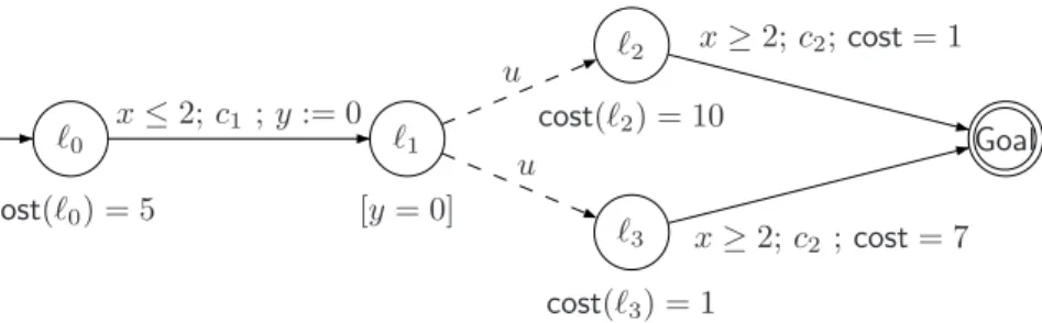
Example 2.2 Consider the RPTGA in Fig.1. Plain arrows represent
control-lable actions (Actc = {c1, c2}) whereas dashed arrows represent uncontrollable
actions (Actu = {u}). Cost rates in locations ℓ0, ℓ2 and ℓ3 are 5, 10 and
1 respectively. In ℓ1 the environment may choose to move to either ℓ2 or ℓ3.
However, due to the invariant y = 0 this choice must be made instantaneously.
2.4 Strategies, Costs of Strategies
Definition 2.3 [Strategy] Let G be a (R)PTGA. A strategy f over G is a
partial function from Runs(G) to Actc∪ {λ}.
Definition 2.4 [Outcome] Let G = (L, ℓ0, Act, X, E, inv, cost) be a (R)PTGA
and f a strategy over G. The outcome Outcome((ℓ, v), f ) of f from configu-ration (ℓ, v) in G is the subset of Runs((ℓ, v), G) defined inductively by:
ℓ0 cost(ℓ0) = 5 ℓ1 [y = 0] ℓ2 cost(ℓ2) = 10 ℓ3 cost(ℓ3) = 1 Goal x≤ 2; c1 ; y := 0 u u x≥ 2; c2; cost = 1 x≥ 2; c2 ; cost = 7
Fig. 1. A Reachability Priced Time Game Automaton A
• (ℓ, v) ∈ Outcome((ℓ, v), f ),
• if ρ ∈ Outcome((ℓ, v), f ) then ρ′ = ρ −→ (ℓe ′, v′) ∈ Outcome((ℓ, v), f ) if
ρ′ ∈ Runs((ℓ, v), G) and one of the following three conditions hold: (i) e ∈ Actu,
(ii) e ∈ Actc and e = f (ρ),
(iii) e ∈ R≥0 and ∀0 ≤ e′ < e,∃(ℓ′′, v′′) ∈ (L × RX≥0) s.t. last(ρ) e′
−−→ (ℓ′′, v′′) ∧
f(ρ−−→ (ℓe′ ′′, v′′)) = λ.
• an infinite run ρ is in ∈ Outcome((ℓ, v), f ) if all the finite prefixes of ρ are
in Outcome((ℓ, v), f ).
A strategy f over a RPTGA G is winning from (ℓ, v) whenever all
max-imal1 runs in Outcome((ℓ, v), f ) are winning. We denote WinStrat((ℓ, v), G)
the set of winning strategies from (ℓ, v) in G. Let f be a winning strategy from configuration (ℓ, v). The cost of f from (ℓ, v) is defined by:
Cost((ℓ, v), f ) = sup{Cost(ρ) | ρ ∈ Outcome((ℓ, v), f )} 2.5 Optimal Control Problems
Let (ℓ0, 0) denote the initial configuration of a RPTGA G. The three main
problems we address in this paper are:
Optimal Cost Computation Problem: we want to compute the optimal cost
one can expect in a RPTGA G from (ℓ0, 0), i.e. to compute
OptCost((ℓ0, 0), G) = inf{Cost((ℓ0, 0), f ) | f ∈ WinStrat((ℓ0, 0), G)}
Optimal Strategy Existence Problem: we want to determine whether the op-timal cost can actually be reached i.e. if there is an opop-timal strategy f ∈ WinStrat((ℓ0, 0), G) such that:
Cost((ℓ0, 0), f ) = OptCost((ℓ0, 0), G)
1
Roughly speaking a run is maximal if it can not be extended in the future by a controllable action (see [6] page 6, section 2.2); this point is discussed in the sequel in section3.2.
Optimal Strategy Synthesis Problem: in case an optimal strategy exists we want to compute a witness.
As the example below shows there are PTGA with no optimal winning strate-gies. In this case there is a family of strategies fε such that
|Cost((ℓ0, 0), fε) − OptCost((ℓ0, 0), G)| < ε
Thus another problem is, given ε, to compute such an fε strategy. This latter
synthesis problem is not dealt with in this paper.
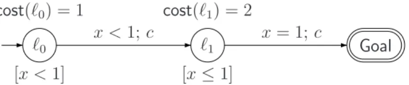
Example 2.5 [No optimal strategy] For the PTGA of Fig. 2 there is no
op-timal strategy. c is a controllable action. Nevertheless we can define a family of strategies fε with 0 < ε ≤ 1 by: f (ℓ0, x < 1 − ε) = λ, f (ℓ0, x= 1 − ε) = c
and f (ℓ1, x ≤ 1) = c. The cost of such a strategy is 1 + ε. So we can get as
close as we want to 1 but there is no optimal winning strategy.
ℓ0 cost(ℓ0) = 1 ℓ1 cost(ℓ1) = 2 Goal x <1; c x= 1; c [x < 1] [x ≤ 1]
Fig. 2. A PTGA with no reachable optimal cost.
Example 2.6 We consider again Fig. 1. We want to compute an optimal
strategy for the controller from the initial configuration. Obviously, once ℓ2 or
ℓ3 has been reached the optimal strategy for the controller is to move to Goal
asap (taking a c2 action). The crucial (and only remaining) question is how
long the controller should wait in ℓ0 before taking the transition to ℓ1 (doing
c1). Obviously, in order for the controller to win this duration must be no more
than two time units. However, what is the optimal choice for the duration in the sense that the overall cost of reaching Goal is minimal? Denote by t the chosen delay in ℓ0. Then 5t + 10(2 − t) + 1 is the minimal cost through ℓ2 and
5t + (2 − t) + 7 is the minimal cost through ℓ3. As the environment chooses
between these two paths the best choice for the controller is to delay t ≤ 2
such that max(21 − 5t, 9 + 4t) is minimum, which is t = 4
3 giving a minimal
cost of 1413. In Fig.3we illustrate the optimal strategy for all states reachable from the initial state provided by our HyTech implementation that will be described in section 3.4.
3
Optimal Cost Computation
In this section we show that computing the optimal cost for a RPTGA amounts
to solving a simple2 control problem on a linear hybrid game automaton [19].
2
Del ay ℓ0→ ℓ1 y 0 x ℓ0 4 3 4 3 2 2 y 0 x ℓi, i ∈ {2, 3} 2 2 Delay ℓi→ Goal
Fig. 3. Optimal strategy for the RPTGA of Fig. 1. Optimal cost is 1413.
As a consequence well-known algorithms [19,8] for computing winning states of reachability hybrid games enable us to compute the optimal cost of a RPTGA. We then show how to use the HyTech tool to implement the computation of the optimal cost for RPTGA.
3.1 From Priced Timed Games to Linear Hybrid Games
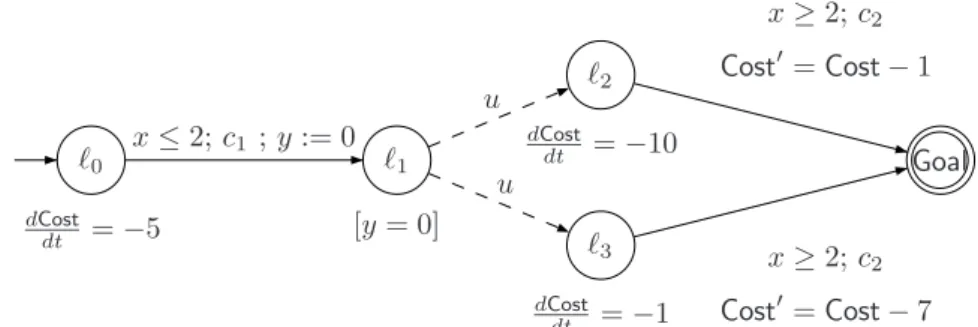
Assume we want to compute the optimal cost of the RPTGA A given in Fig.1.
We translate this automaton into a linear hybrid game automaton (LHGA for
short) H (see Fig. 4) where the cost function is encoded into a variable Cost
of the LHGA. In H the variable Cost decreases with rate k in a location ℓ (i.e.
dCost
dt = −k in ℓ) if Cost(ℓ) = k in A. As for discrete transitions the variable
Costis updated by Cost′ = Cost − k in H if the corresponding transition’s cost in A is k. ℓ0 dCost dt = −5 ℓ1 [y = 0] ℓ2 dCost dt = −10 ℓ3 dCost dt = −1 Goal x≤ 2; c1 ; y := 0 u u x≥ 2; c2 Cost′= Cost − 1 x≥ 2; c2 Cost′= Cost − 7 Fig. 4. The Linear Hybrid Game Automaton H.
Let CompWin be a semi-algorithm (e.g. [19,8]) that computes the largest set of winning states for a reachability hybrid game. Using CompWin we can compute the largest set of winning states for H with the goal states given by
Goal∧Cost ≥ 0. The meaning of this new reachability game is that we want to
win without having spent all the resources (Cost) we started with. Assume the corresponding (largest) set of winning states is denoted CompWin(H, Goal ∧
Cost≥ 0). The meaning of the set W = CompWin(H, Goal ∧ Cost ≥ 0) is that
in order to win one has to start in the region given by W and if one starts outside W the opponent has a strategy to win i.e. we lose. We can prove
(see [6], Theorem 5 and Lemma 6) that the (largest) set of winning states
W is a union of zones of the form (ℓ, R ∧ Cost ≻ h) where ℓ is a location,
R ⊆ RX
≥0, h is a piece-wise affine function on R and ≻∈ {>, ≥}. Hence we
have the answer to the optimal reachability game: we intersect the set of initial states with the set of winning states W , and in case it is not empty, the projection on the Cost axis yields a constraint on the cost like Cost ≻ k
with k ∈ Q≥0 and ≻∈ {>, ≥}. By definition of the winning set of states in
reachability games, this is the largest set from which we can win, no cost lower than or equal to k is winning and we can deduce that k is the optimal cost. Also we can decide whether there is an optimal strategy or not: if ≻ is equal to > there is no optimal strategy and if ≻ is ≥ there is one.
Thus computing CompWin(H, Goal ∧ Cost ≥ 0) is a semi-algorithm for computing the optimal cost of the RPTGA A. Moreover we can decide (if
CompWinterminates) whether there exists an optimal strategy or not: in case
the initial winning cost set is of the form Cost > k there is no optimal strategy
but a family of strategies fε (for ε > 0) with cost lower than k + ε. When
this set if of the form Cost ≥ k (and assuming CompWin terminates) we can
compute an optimal strategy (this point is dealt with in the next section 4).
The formal definitions and proofs of this reduction are given in [6] (Defi-nition 12, Lemma 5, Theorems 4 and 5, Corollaries 1 and 2).
3.2 The π Operator
The computation of the winning states (with CompWin) is based on the defini-tion of a controllable predecessor operator [16,8]. Let G = (L, ℓ0, Act, X, E, inv,
cost) be a RPTGA and Q its set of configurations. For a set X ⊆ Q and
a ∈ Act we define Preda
(X) = {q ∈ Q | q −−→ qa ′, q′ ∈ X}. The
control-lable and uncontrolcontrol-lable discrete predecessors of X are defined by cPred(X) = S c∈ActcPred c (X), respectively uPred(X) =S u∈ActuPred u (X). We also need a notion of safe timed predecessors of a set X w.r.t. a set Y . Intuitively a state q is in Predt(X, Y ) if from q we can reach q′ ∈ X by time elapsing and along
the path from q to q′ we avoid Y . Formally this is defined by:
Predt(X, Y ) = {q ∈ Q | ∃δ ∈ R≥0 s.t. q δ
−→ q′, q′ ∈ X ∧ Post[0,δ](q) ⊆ Y } (1)
where Post[0,δ](q) = {q′ ∈ Q | ∃t ∈ [0, δ] | q t
−→ q′}. We are then able to define
a controllable predecessor operator π as follows:
π(X) = Predt¡X ∪ cPred(X), uPred(X)
¢
(2) This definition of π captures the choice that uncontrollable actions cannot be used to win (this choice is made in [13] and in [6]). As a matter of fact there is
no way to win in the RPTGA of Fig. 1with this definition of π: ℓ1 cannot be
a winning state if we start iterating the computation of π from Goal as π only adds predecessors that can reach a winning state by a controllable transition.
Another choice is possible: uncontrollable actions may be used to win if they are forced to happen. This second choice is rather involved when one wants to give a new definition of π in the general case. We adopt a position which is half-way between the previous two extremes: if an uncontrollable action is enabled from a state q where time cannot elapse and leads to a winning
state q′, and no uncontrollable transitions enabled at q can lead to a
non-winning state, we declare q as non-winning. Assume the set of configurations of G where time cannot elapse is denoted STOP . Then a new definition of π where uncontrollable actions can be used to win is given by:
π′(X) = Predt¡X ∪ cPred(X) ∪ (uPred(X) ∩ STOP), uPred(X)¢ (3)
Note that this choice does not change the results presented in [6]. In the example of Fig.1, from location ℓ1only uncontrollable transitions are enabled,
but they are bound to happen within a bounded amount of time (in this case as soon as we reach ℓ1because of the invariant y = 0). π′ will add configuration
(ℓ1, x≥ 0 ∧ y = 0) to the set of winning states.
The semi-algorithm CompWin computes the least fixed point W of the functional λX.{X0} ∪ π′(X) as the limit of an increasing sequence of sets of
states Wi (starting from set W0 = X0) where Wi+1 = π′(Wi)). If G is a
RPTGA, the result of the computation of CompWin on the associated LHGA
H starting from Goal ∧ Cost ≥ 0 is W = µX.{Goal ∧ Cost ≥ 0} ∪ π′(X). This
result is also denoted CompWin(H, Goal ∧ Cost ≥ 0) and gives the largest set of winning states.
3.3 Termination Issues
An important issue about the previous semi-algorithm CompWin is whether it terminates or not. We have identified a class of RPTGA for which CompWin terminates on the associated hybrid game.
Let G be a RPTGA satisfying:
• G is bounded, i.e. all clocks in G are bounded3;
• the cost function of G is strictly non-zeno, i.e. there exists some κ > 0 such
that the accumulated cost of every cycle in the region automaton associated with G is at least κ. Note that this condition can be checked. For more complete explanations, see [6].
Then the semi-algorithm CompWin(H, Goal ∧ Cost ≥ 0) terminates (H is the hybrid game defined from G in the previous section). The formal statement and proof of this claim is given by Theorem 6 in [6]. We thus get:
Theorem 3.1 Let G be a RPTGA satisfying the above-mentionned hypothe-ses (boundedness and strict non-zenoness of the cost). Then the optimal cost is computable for G.
3
3.4 Implementation of CompWin in HyTech
HyTech[10,11] is a tool that implements “pre” and “post” operators for linear
hybrid automata. Moreover it is possible to write programs that use these operators (and many others) on polyhedra in order to compute sets of states.
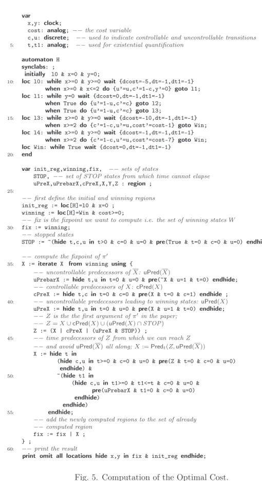
The specification in HyTech of our LHGA H of Fig. 4 is given in Fig. 5,
lines 7–20. We detail this specification in the sequel.
Controllable and Uncontrollable Predecessors. HyTech provides the pre operator that computes at once the time predecessors and the discrete prede-cessors of a set of states. As we need to distinguish between time predeprede-cessors, discrete controllable predecessors and discrete uncontrollable predecessors, we use the following trick: in the HyTech source code of the LHA H we add
two boolean variables u and c (Fig. 5, line 4) that are negated on each
dis-crete uncontrollable (resp. controllable) transitions (Fig. 5, lines 10–19). In
HyTechone can existentially quantify over a variable t by using the hide
op-erator. Then the controllable predecessors can be computed by existentially
quantifying over c and over a variable t that has rate4 −1. We can express
the cPred (and uPred) operator with existential quantifiers and two variables t and c as follows: cPred(X) = {q | ∃c ∈ Actc s.t. q c − → q′, q′ ∈ X} = {q | ∃t s.t. ∃c s.t. t = 0 ∧ c = 0 ∧ (q, t, c) ∈ pre(X ∧ t = 0 ∧ c = 1)} where pre is the predecessor operator of HyTech.
We impose that the value of t stays unchanged to ensure that we just take discrete predecessors (Fig.5, line39). For uncontrollable predecessors we
replace c by u (Fig. 5, line 41). Note that the computation of STOP states
(Fig. 5, line 32) can also be done using our extra variables t, c, u.
Safe Time Predecessors. The other operator Predt(Z, Y ) is a bit more
com-plicated. We just need to express it with existential quantification so that it is easy to compute it with HyTech. Also we assume we have time determin-istic automata as in this case Predt(Z, Y ) is rather simple (if we do not have
time determinism a more complicated encoding must be done and we refer the reader to [19] for a detailed explanation.) From equation (1) we get:
Predt(Z, Y ) = {q | ∃t ≥ 0 s.t. q t − → q′, q′ ∈ Z and ∀0 ≤ t1 ≤ t, q t − → q′′ =⇒ q′′6∈ Y } = {q | ∃t ≥ 0 s.t. q−→ qt ′, q′ ∈ Z and ¬(∃0 ≤ t1 ≤ t, q t − → q′′∧ q′′∈ Y )}
The latter formula can be encoded in HyTech using the hide operator (Fig.5,
lines 47–55) and two auxiliary variables t and t1 that evolves at rate −1 (note
4
any rate different from 0 would also do but we need another variable t with rate −1 later on and use this one.
var
x,y: clock;
cost: analog; −− the cost variable
c,u: discrete; −− used to indicate controllable and uncontrollable transitions 5: t,t1: analog; −− used for existential quantification
automaton H synclabs: ;
initially l0 & x=0 & y=0;
10: loc l0: while x>=0 & y>=0 wait {dcost=-5,dt=-1,dt1=-1} when x>=0 & x<=2 do {u’=u,c’=1-c,y’=0} goto l1; loc l1: while y=0 wait {dcost=0,dt=-1,dt1=-1}
when True do {u’=1-u,c’=c} goto l2; when True do {u’=1-u,c’=c} goto l3;
15: loc l3: while x>=0 & y>=0 wait {dcost=-10,dt=-1,dt1=-1} when x>=2 do {c’=1-c,u’=u,cost’=cost-1} goto Win; loc l4: while x>=0 & y>=0 wait {dcost=-1,dt=-1,dt1=-1}
when x>=2 do {c’=1-c,u’=u,cost’=cost-7} goto Win; loc Win: while True wait {dcost=0,dt=-1,dt1=-1}
20: end
var init_reg,winning,fix, −− sets of states
STOP, −− set of STOP states from which time cannot elapse
uPreX,uPrebarX,cPreX,X,Y,Z : region ;
25:
−− first define the initial and winning regions
init_reg := loc[H]=l0 & x=0 ; winning := loc[H]=Win & cost>=0;
−− fix is the fixpoint we want to compute i.e. the set of winning states W 30: fix := winning;
−− stopped states
STOP := ~(hide t,c,u in t>0 & c=0 & u=0 & pre(True & t=0 & c=0 & u=0) endhide) ;
−− compute the fixpoint of π′ 35: X := iterate X from winning using {
−− uncontrollable predecessors of X: uPred(X)
uPrebarX := hide t,u in t=0 & u=0 & pre(~X & u=1 & t=0) endhide;
−− controllable predecessors of X: cPred(X)
cPreX := hide t,c in t=0 & c=0 & pre(X & t=0 & c=1) endhide ;
40: −− uncontrollable predecessors leading to winning states: uPred(X)
uPreX := hide t,u in t=0 & u=0 & pre(X & u=1 & t=0) endhide;
−− Z is the the first argument of π′in the paper; −− Z = X ∪ cPred(X) ∪ (uPred(X) ∩ STOP)
Z := (X | cPreX | (uPreX & STOP)) ;
45: −− time predecessors of Z from which we can reach Z −− and avoid uPred(X) all along; X := Predt(Z, uPred(X))
X := hide t in
(hide c,u in t>=0 & c=0 & u=0 & pre(Z & t=0 & c=0 & u=0) endhide) &
50: ~(hide t1 in
(hide c,u in t1>=0 & t1<=t & c=0 & u=0 & pre(uPrebarX & t1=0 & c=0 & u=0) endhide)
endhide)
55: endhide;
−− add the newly computed regions to the set of already −− computed region
fix := fix | X ; } ;
60: −− print the result
print omit all locations hide x,y in fix & init_reg endhide;
that those variables are not part of the model but only used in existentially quantified formulas and they do not constrain the behavior of H.) Finally if the computation of π′ terminates (Fig.5, lines35–59) the set fix contains all
the winning states. It then suffices to compute the projection on cost in the initial state to obtain the optimal cost (Fig. 5, line 61).
Doing this we have solved the first two problems: computing the optimal cost and deciding whether there exists an optimal strategy.
4
Optimal Strategies Computation
In this section we show how to compute an optimal strategy when one exists. Then we give the HyTech implementation of this computation and discuss some properties of those strategies.
4.1 Strategy Synthesis For RPTGA
First we recall some basic properties of strategies for (unpriced) Timed Game Automata (TGA).
A strategy f is
• state-based whenever ∀ρ, ρ′ ∈ Runs(G), last(ρ) = last(ρ′) implies that f (ρ) =
f(ρ′). State-based strategies are also called memoryless strategies in game
theory [18,8];
• polyhedral if for all a ∈ Actc ∪ {λ}, f−1(a) is a finite union of convex
poly-hedra for each location of the game;
• realizable, whenever the following holds: for all ρ ∈ Outcome(q, f ) s.t. f
is defined on ρ and f (ρ) = λ, there exists some δ > 0 such that for all 0 ≤ t < δ, there exists q′ with ρ−→ qt ′ ∈ Outcome(q, f ) and f (ρ −→ qt ′) = λ.
Strategies which are not realizable are not interesting because they generate empty sets of outcomes. Nevertheless it is not clear from [16,4] how to extract strategies for RPTGA and ensure their realizability as shown by the following example.
ℓ0 Goal
x >1; c
Fig. 6. A timed game automaton
Example 4.1 Consider the PTGA of Fig. 6where c is a controllable action.
The game is to enforce state Goal. The most natural strategy f would be to do a c when x > 1 and to wait until x reaches a value greater than 1. Formally this yields f (ℓ0, x ≤ 1) = λ and f (ℓ0, x > 1) = c. This strategy is
not realizable. In the sequel, we build a strategy which is f (ℓ0, x < 2) = λ and
this case we start with the following strategy (not realizable): f (ℓ0, x≤ 1) = λ
and f (ℓ0,1 < x ≤ 2) = c. To make it realizable we will take the first half
of 1 < x ≤ 2 and have a delay action on it i.e. f (ℓ0, x < 32) = λ and
f(ℓ0,32 ≤ x ≤ 2) = c. In the following, we will restrict our attention to
realizable strategies and simply refer to them as strategies.
A secondary result is provided in [6] for Linear Hybrid Games (Theorem 2 page 7) that can be rephrased in the context of RPTGA as:
Theorem 4.2 (Adapted from Theorem 2 of [6]) Let G be a RPTGA. If the semi-algorithm CompWin terminates for the hybrid game associated with G
(see section 3.1), then we can compute a winning strategy which is: polyhedral,
realizable and stated-based.
Let H be the LHGA associated to the RPTGA G = (L, ℓ0, Act, X, E, inv, cost).
A state of H is a triple (ℓ, v, c) where ℓ ∈ L, v ∈ RX
≥0 and c ≥ 0 (c is the value of
the variable Cost of H). Thus if we synthetize a realizable winning state-based strategy f for H, we obtain a strategy that depends on the cost value. In case there is a winning strategy for H (see section3.1) we can synthetize realizable state-based winning strategies for G (see [6], Corollary 2). This result is already satisfying but we would like to build strategies that are independent of the cost value i.e. in which there is no need for extra information to play the strategy on the original RPTGA G (this means we want to build a state-based strategy for the original RPTGA G.) To this extent we introduce the notion of cost-independent strategies.
Let W = CompWin(H, Goal ∧ Cost ≥ 0) be the set of winning states of H. A state-based strategy f for H is cost-independent if (ℓ, v, c) ∈ W and (ℓ, v, c′) ∈ W implies f (ℓ, v, c) = f (ℓ, v, c′). Cost-independent strategies in H
will then be used for having state-based strategies in G. Theorem 7 of [6] gives then sufficient conditions for the existence of a state-based, optimal, realizable strategy in G and, when back to the automaton reads as follows:
Theorem 4.3 (Adapted from Theorem 7 of [6]) Let G be a RPTGA. H is the associated LHGA. If CompWin terminates for H and the set of winning states is W = CompWin(H, Goal ∧ Cost ≥ 0) is a union of sets of the form
(ℓ, R ∧ Cost ≥ h) where ℓ is a location, R ⊆ RX
≥0 and h is a piece-wise affine
function on R, then there exists a winning realizable state-based strategy f
defined over WG = ∃Cost.W s.t. for each q ∈ WG, f ∈ WinStrat(q, WG) and
Cost(q, f ) = OptCost(q).
Note that under the previous conditions we build a strategy f which is
uniformly optimal i.e. optimal for all states of WG. A syntactical criterion
to enforce the condition of theorem 4.3 is that the constraints (guards) on
controllable actions are non-strict and constraints on uncontrollable actions are strict. We now give an algorithm to extract such an optimal, state-based, realizable and winning strategy for a RPTGA G.
we can compute an optimal strategy for this model. Moreover, the strategy
we obtain using HyTech is precisely the one we described in Fig. 3.
4.2 Synthesis of Optimal Strategies
The set of winning states of H is computed iteratively using the functional π′
defined by equation (3). In the sequel we need to compute the states that can let a strict positive delay elapse to define the strategy for the delay action. For a set X we denote NonStop(X) the set of states in X from which a strict positive delay can elapse and all the intermediary states lie in X i.e.
NonStop(X) = {q ∈ X | ∃t > 0 | q + t ∈ X ∧ ∀0 ≤ t′ ≤ t, q + t′ ∈ X} (4)
Tagged Sets. To synthetize strategies we compute iteratively a set of extended
“tagged” states W+ during the course of the computation of W (this follows
from Theorem 2 and Lemma 6 of [6]). The tags will contain information about
how a new set of winning states Wi+1 = π′(Wi) has been obtained.
We start with W0+ = ∅ and W0 = Goal ∧ Cost ≥ 0. Assuming Wi and Wi+
are the sets obtained after i iterations of π′ we define Wi+1+ as follows: (i) let Y = Wi+1\ Wi where Wi+1 = π′(Wi);
(ii) for each c ∈ Actc, we define the tagged set
³
Y ∩ cPredc(W i)
´[c]
with the
intended meaning: “Y ∩ cPredc(Wi) has been added to the set of winning
states by a Predc and doing a c from this set leads to Wi”;
(iii) define another tagged set ³NonStop(Y )´[λ] with the intended meaning:
“NonStop(Y ) has been added to the set of winning states by the (strictly positive) time predecessors operator and letting time elapse will lead to either Wi or cPred(Wi) or uPred(Wi) ∩ STOP ”;
(iv) define Wi+1+ by :
Wi+1+ = Wi+∪³NonStop(Y )´[λ]∪ [
c∈Actc ³
Y ∩ cPredc(Wi)
´[c]
Computation of an Optimal Strategy. If CompWin terminates in j iterations
we end up with W+ = W+
j . Note that by construction a state q of W may
belong to several tagged sets X0[λ], X [c1]
1 , . . . , X [cn]
n (where ci ∈ Actc for each
i ∈ [1, n]) of W+. If the assumptions of theorem 4.3 are satisfied all the X i’s
are of the form X′
i ∧ Cost ≥ hi where Xi′ ⊆ {ℓi} × RX≥0 for some location ℓi
and hi : Xi′ → R≥0 is a piecewise affine function. Thus the infimum of hi over
Xi′ is reachable and equal to the minimum of hi.
Theorem 7 of [6] states that in this case an optimal state-based strategy
optimal choice: let m = mini∈[0,n]hi(q); then defining f∗(q) = ci if hi(q) = m
gives an optimal strategy.
As it can be the case that hi(q) = hj(q) = m with i 6= j, we impose a
total order ⊏ on the set of events in Actc and define f∗(q) = ci where i =
max{j | hj(q) = m}. To avoid realizability problems (see proof of Lemma 6
in [6]) on the boundary of a set Xi if h0(q) = m (which means that the optimal
cost can be achieved by time elapsing) and hi(q) = m for some i ∈ [1, n] we
define f∗(q) = c
i. This can be easily defined in our setting by extending ⊏ to
Actc∪ {λ} and making λ the smallest element.
After these algorithmics explanations, we can summarize how we can syn-thesize an optimal, cost-independent strategy. We denote W[c]+ the set defined by:
W[c]+ = [
Si[c]∈W+
Si (5)
For each c ∈ Actc ∪ {λ}, W[c]+ is a set of the form Xc ∧ Cost ≥ hc where
hc is a piecewise affine function on Xc (Xc is a union of convex polyhedra).
Note that the constraint Cost ≥ hc is a polyhedron which constrains the Cost
variable and the clocks. In what follows, a pair (q, α) will represent a state of H (α is the value of the Cost variable). For each winning state q of G, we want to compute the minimal cost for winning and which action we should do if we want to win with the optimal cost. Let us consider two actions c1, c2 ∈ Actc∪ {λ}. We denote [c1 ≤ c2] the set of winning states of G where
it is better to do action c1 than action c2 (hc1(q) ≤ hc2(q)). This set is defined
by: [c1 ≤ c2] = {q ∈ Xc1 | ∃α1| (q, α1) ∈ W[c+1] and ∀α2| (q, α2) ∈ W[c+2], α1 ≤ α2} (6) =©q ∈ Xc1 | ∃α 1| (q, α1) ∈ W[c+1]∧ ¬¡∃α2| (q, α2) ∈ W[c+2] and α2 < α1 ¢ª (7)
Each set [c1 ≤ c2] is a polyhedral set. For each c ∈ Actc∪ {λ} define
Opt(c) = \
c′6=c
[c ≤ c′] (8)
Opt(c) is the set of states for which c is an action that gives the optimal cost.
W∗ = S
c∈Actc∪{λ}Opt(c) is thus equal to the set of states on which we need
to define the optimal strategy. Given the total order ⊏ on Actc ∪ {λ} with
λ ⊏ c1 ⊏ · · · ⊏ cn, we can define an optimal strategy f∗ as follows: for
i ∈ [0, n − 1], let Bi = ¡W∗ \ (∪k>iBk)¢ ∩ Opt(ci) and Bn = W∗ ∩ Opt(cn);
define then f∗(q) = c
i if q ∈ Bi. f∗ is an optimal strategy that is (winning),
4.3 Implementation in HyTech
Controllable Tagged Sets. We first show how to compute tagged sets of states. Our HyTech encoding consists in adding a discrete variable a to the
HyTech model of Fig. 5and use it in the guards of controllable transitions:
controllable action ck of Fig.4corresponds to the guard a = k in the HyTech
model. The HyTech model of Fig. 5is enriched as follows: we add the guard
a= 1 to line 11, a = 2 to lines16and18. In this way we achieve the tagging of
controllable predecessors as now the computation of cPred (line 39 of Fig. 7)
will compute a tagged region that will be a union of polyhedra with some
a = k constraints. Note that we also modify line 44 of Fig. 5 and replace it
by line 20in Fig. 7where a is hidden from the new cPreX as a is not needed
to compute the winning set of states.
New NonStop States. To compute NonStop(Y ) we use again our extra
vari-ables t, c, u and add the tag a = 0 to the result set. Lines 35–36 of Fig. 7
achieves this.
W+ is stored in the region fix_strat in the HyTech code. To compute
Wi+1+ we update fix_strat as described by line38 in Fig. 7.
Computation of the Optimal Strategy. To compare the costs for each action and determine the optimal one we use the trick described in the previous subsection. Each tagged set gives the function hci by the means of a constraint
between the Cost variable and the rest of the state variables. To compute hci
we need to split the state space according to each action ci: this is achieved
by lines 44–46 where the state space that corresponds to hci is stored in ri. It remains to compute for each pair of actions (c1, c2) (ci can be λ), the set
[c1 ≤ c2] states. The encoding in HyTech of the formula given by equation (7)
is quite straightforward using the hide operator that corresponds to existential quantification. The strategy is then computed as described at the end of the
previous subsection by lines 54–63.
5
Experiments
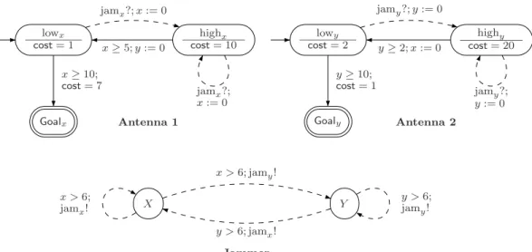
Using a HyTech-code as described in this paper, we have done some more experiments. The most important example we have treated is a model of a mobile phone with two antennas trying to connect to a base station with an environment which can possibly jam some transmissions.
Description of the Mobile Phone Example. We consider a mobile phone with two antennas emitting on different channels. Making the initial con-nection with the base station takes 10 time units whatever antenna is in use. Statistically, a jam of the transmission (e.g. collision with another phone) may appear every 6 time units in the worst case. When a collision is observed, the antenna tries to transmit with a higher level of energy for a while (at least 5
var
−− same set of variables here as lines22–24in Fig.5plus some new vars:
a: discrete; cost0,cost1,cost2: analog; 5: fix_strat,nonstop,Y, r0,r1,r2, B0,B1,B2, inf_0_1,inf_0_2,inf_1_0,inf_1_2,inf_2_0,inf_2_1: region;
10: init_reg := loc[H]=l0 & x=0 ; winning := loc[H]=Win & cost>=0; fix := winning;
STOP := ~(hide t,c,u in t>0 & c=0 & u=0 & pre(True & t=0 & c=0 & u=0) endhide) ; fix_strat := False; −− this is new and corresponds to W0+= ∅
15:
X := iterate X from winning using {
uPrebarX := hide t,u in t=0 & u=0 & pre(~X & u=1 & t=0) endhide; cPreX := hide t,c in t=0 & c=0 & pre(X & t=0 & c=1) endhide ; uPreX := hide t,u in t=0 & u=0 & pre(X & u=1 & t=0) endhide;
20: Z := (X | (hide a in cPreX endhide) | (uPreX & ~uPrebarX & STOP)) ; X := hide t in
(hide c,u in t>=0 & c=0 & u=0 & pre(Z & t=0 & c=0 & u=0) endhide) &
~(hide t1 in
25: (hide c,u in t1>=0 & t1<=t & c=0 & u=0 & pre(uPrebarX & t1=0 & c=0 & u=0) endhide)
endhide) endhide;
30:
Y := X & ~fix ; −− store the real new states in Y
fix := fix | X ;
−− computation of NonStop(Y ) 35: nonstop := a=0 & Y &
hide t,c,u in t>0 & c=0 & u=0 & pre(Y & t=0 & u=0 & c=0) endhide;
−− computation of fix_strat
fix_strat := fix_strat | (Y & cPreX) | nonstop ; } ;
40: −− print the result as before
print omit all locations hide x,y in fix & init_reg endhide;
−− rename the cost fonction; then ri corresponds to hci
r0 := hide a,cost in cost0=cost & fix_strat & a=0 endhide ;
45: r1 := hide a,cost in cost1=cost & fix_strat & a=1 endhide ; r2 := hide a,cost in cost2=cost & fix_strat & a=2 endhide ;
−− compute the state space inf_i_j where hci(q) ≤ hcj(q)
inf_0_1 := hide cost0 in r0 & ~(hide cost1 in r1 & cost1<cost0 endhide) endhide ;
50: ...
inf_2_1 := hide cost2 in r2 & ~(hide cost1 in r1 & cost1<cost2 endhide) endhide ;
−− Output the result taking the best move according to the total order (Actc∪ {λ}, ⊏)
prints "Optimal Winning Strategy" ;
55: prints "do control from l3 or l4 to Win (a=2) on"; B2 := inf_2_0 & inf_2_1 ;
print B2 ;
prints "do control from l0 to l1 (a=1) on"; B1 := inf_1_0 & inf_1_2 & ~B2 ;
60: print B1 ;
prints "do wait (a=0) on";
B0 := inf_0_1 & inf_0_2 & ~B1 & ~B2 ; print B0;
time units for Antenna 1 and at least 2 time units for Antenna 2) and then can switch back to the lower consumption mode. Unfortunately, switching back to the low consumption mode requires more resources and forces to interrupt the other transmission (Antenna 1 resets variable y of Antenna 2 and vice-versa). The overall cost rate (consumption per time unit) for the mobile phone in a
product state s = (lowx,highy,Y) is the sum of the rates of Antenna 1 and
Antenna 2 (both are working) i.e. 1 + 20 = 21 and Cost(s) = 21 in our model. Once the connection with the base station is established (either x ≥ 10 or
y ≥ 10) the message is delivered with an energy consumption depending on
the antenna (Cost = 7 for Antenna 1 and Cost = 1 for Antenna 2). The aim
is to connect the mobile phone with an energy consumption (cost) as low as possible whatever happens in the network (jam).
Antenna 1 lowx cost= 1 highx cost= 10 Goalx jamx?; x := 0 x≥ 5; y := 0 x≥ 10; cost= 7 jamx?; x:= 0 Antenna 2 lowy cost= 2 highy cost= 20 Goaly jamy?; y := 0 y≥ 2; x := 0 y≥ 10; cost= 1 jamy?; y:= 0 Jammer X Y x >6; jamy! y >6; jamx! x >6; jamx! y >6; jamy!
Fig. 8. Mobile Phone Example.
This system can be represented by a network of PTGAs (see Fig.8where
plain arrows represent controllable actions whereas dsahed arrows represent uncontrollable actions) and the problem reduces to finding an optimal strategy for reaching one of the goal states Goalx or Goaly. Note that our original model
is a single PTGA and not a network of PTGAs, but networks of PTGA can be used as well because it does not add expressive power and it is simple to define the composed PTGA: in a global location (being a tuple of locations of simple PTGAs), the cost is simply the sum of the costs of all single locations composing it. Idem for a composed transition resulting from a synchroniza-tion: the cost of the synchronized transition is the sum of the costs of the two initial transitions. Of course, one has to pay attention that no control-lable action can synchronize with an uncontrolcontrol-lable action in order that we can define properly the nature, controllable or not, of the synchronization. In this example, see Fig. 8, jamx? (resp. jamy?) synchronizes with jamx! (resp.
jamy!). The HyTech code of this example can be found in [6] and on the
web page http://www.lsv.ens-cachan.fr/aci-cortos/ptga/.
y 0 x highx.highy.Y 5 5 10 10 y= − 5 3 x + 6 y= x y= 2 y 0 x highx.highy.X 6 10 4 y= x+ 6 y 0 x highx.lowy.Y 10 5 10 2 (10, 20) (10, 12) y= x+ 10 y= x+ 2 y 0 x highx.lowy.X 10 10 y 0 x lowx.highy.Y 10 10 14 3 2 y 0 x lowx.lowy.Y y= x+ 10 y= x+ 2 y= x− 5 y= x− 10 10 10 low x→ Go al o rlo wy → Go al Del ay y 0 x lowx.lowy.X y= x− 5 y= x− 10 10 10 Delay highx→lowx highy→lowy lowx→Goalx lowy→Goaly
Fig. 9. Optimal Strategy for the Mobile Phone Example
Results of our Experiments. We got that the optimal cost (lowest energy consumption) that can be ensured is 109. The optimal strategy is graphically
represented on Fig. 9. The strategy is non-trivial and the actions to take
depend on a complex partitioning of the clock space. The computation took 828s on a 12” PowerBook G4 running Mac OS X.
6
Conclusion
In this paper we have described an algorithm to synthesize optimal strategies for a sub-class of priced timed game automata. The algorithm is based on the work described in [6] where we proved this problem was decidable (under some hypotheses we recall in this paper). Morever, we also provide an implemen-tation of our algorithm in HyTech and demonstrate it on small case-studies. In a recent paper [2] Alur et al. addressed a related problem i.e. “compute the optimal cost within k steps”. They give a complexity bound for this restricted “bounded” problem and prove that the splitting incurred by the computation of the optimal cost within k steps only yields an exponential number (in k and the size of the automaton) of subregions. They do not consider the problem of strategy synthesis.
Our future work consists in extending the class of systems for which the algorithm we provided terminates. The synthesis of sub-optimal strategies (when no optimal strategy exists) is currently being investigated. We would also like to extend this work to more general winning conditions (like safety conditions) and with other performance criteria (as for example the price per unit of time along infinite schedules).
References
[1] Y. Abdeddaim. Modélisation et résolution de problèmes d’ordonnancement à l’aide d’automates temporisés. PhD thesis, Institut National Polytechnique de Grenoble, Grenoble, France, 2002.
[2] R. Alur, M, Bernadsky, and P. Madhusudan. Optimal reachability in weighted timed games. In Proc. 31st International Colloquium on Automata, Languages and Programming (ICALP’04), Lecture Notes in Computer Science. Springer, 2004. To appear.
[3] R. Alur, S. La Torre, and G.J. Pappas. Optimal paths in weighted timed automata. In Proc. 4th International Workshop on Hybrid Systems: Computation and Control (HSCC’01), volume 2034 of Lecture Notes in Computer Science, pages 49–62. Springer, 2001.
[4] E. Asarin, O. Maler, A, Pnueli, and J. Sifakis. Controller synthesis for timed automata. In Proc. IFAC Symposium on System Structure and Control, pages 469–474. Elsevier Science, 1998.
[5] G. Behrmann, A. Fehnker, T. Hune, K.G. Larsen, P. Pettersson, Judi Romijn, and Frits Vaandrager. Minimum-cost reachability for priced timed automata. In Proc. 4th International Workshop on Hybrid Systems: Computation and Control (HSCC’01), volume 2034 of Lecture Notes in Computer Science, pages 147–161. Springer, 2001.
[6] P. Bouyer, F. Cassez, E. Fleury, and K.G. Larsen. Optimal strategies in priced timed game automata. Research Report BRICS RS-04-4, Denmark, Feb. 2004. Available at http://www.brics.dk/RS/04/4/.
[7] E. Brinksma, A. Mader, and A. Fehnker. Verification and optimization of a PLC control schedule. Journal of Software Tools for Technology Transfer (STTT), 4(1):21–33, 2002.
[8] L. de Alfaro, T.A. Henzinger, and R. Majumdar. Symbolic algorithms for infinite-state games. In Proc. 12th International Conference on Concurrency Theory (CONCUR’01), volume 2154 of Lecture Notes in Computer Science, pages 536–550. Springer, 2001.
[9] A. Fehnker. Scheduling a steel plant with timed automata. In Proc. 6th International Conference on Real-Time Computing Systems and Applications (RTCSA’99), pages 280–286. IEEE Computer Society Press, 1999.
[10] T.A. Henzinger, P.-H. Ho, and H. Wong-Toi. A user guide to hytech. In Proc. 1st International Conference on Tools and Algorithms for the Construction and Analysis of Systems (TACAS’95), volume 1019 of Lecture Notes in Computer Science, pages 41–71. Springer, 1995.
[11] T.A. Henzinger, P.-H. Ho, and H. Wong-Toi. HyTech: A model-checker for hybrid systems. Journal on Software Tools for Technology Transfer (STTT), 1(1–2):110–122, 1997.
[12] T. Hune, K.G. Larsen, and P. Pettersson. Guided synthesis of control programs using uppaal. In Proc. IEEE ICDS International Workshop on Distributes Systems Verification and Validation, pages E15–E22. IEEE Computer Society Press, 2000.
[13] S. La Torre, S. Mukhopadhyay, and A. Murano. Optimal-reachability and control for acyclic weighted timed automata. In Proc. 2nd IFIP International Conference on Theoretical Computer Science (TCS 2002), volume 223 of IFIP Conference Proceedings, pages 485–497. Kluwer, 2002.
[14] K.G. Larsen. Resource-efficient scheduling for real time systems. In Proc. 3rd International Conference on Embedded Software (EMSOFT’03), volume 2855 of Lecture Notes in Computer Science, pages 16–19. Springer, 2003. Invited presentation.
[15] K.G. Larsen, G. Behrmann, E. Brinksma, A. Fehnker, T. Hune, P. Pettersson, and J. Romijn. As cheap as possible: Efficient cost-optimal reachability for priced timed automata. In Proc. 13th International Conference on Computer Aided Verification (CAV’01), volume 2102 of Lecture Notes in Computer Science, pages 493–505. Springer, 2001.
[16] O. Maler, A. Pnueli, and J. Sifakis. On the synthesis of discrete controllers for timed systems. In Proc. 12th Annual Symposium on Theoretical Aspects of Computer Science (STACS’95), volume 900 of Lecture Notes in Computer Science, pages 229–242. Springer, 1995.
[17] P. Niebert and S. Yovine. Computing efficient operations schemes for chemical plants in multi-batch mode. European Journal of Control, 7(4):440–453, 2001. [18] W. Thomas. On the synthesis of strategies in infinite games. In Proc. 12th
Annual Symposium on Theoretical Aspects of Computer Science (STACS’95), volume 900, pages 1–13. Springer, 1995. Invited talk.
[19] H. Wong-Toi. The synthesis of controllers for linear hybrid automata. In Proc. 36th IEEE Conference on Decision and Control, pages 4607–4612. IEEE Computer Society Press, 1997.

![[PDF] Introduction à la conception objet et à c++ | Cours informatique](data:image/gif;base64,R0lGODlhAQABAIAAAP///wAAACH5BAEAAAAALAAAAAABAAEAAAICRAEAOw==)