OATAO is an open access repository that collects the work of Toulouse
researchers and makes it freely available over the web where possible
Any correspondence concerning this service should be sent
to the repository administrator:
[email protected]
This is an author’s version published in: http://oatao.univ-toulouse.fr/26544
To cite this version:
Oberlin, Thomas
and Malgouyres, François
and Wu, Jin-Yi
Loss functions for denoising compressed images: a comparative
study. (2019) In: 27th European Signal Processing Conference
(EUSIPCO 2019), 2 September 2019 - 6 September 2019 (A
Coruña, Spain).
Official URL:
1st Thomas Oberlin INP–ENSEEIHT and IRIT
Université de Toulouse Toulouse, France [email protected]
2nd François Malgouyres Institut de Mathématiques de Toulouse UMR5219, Université de Toulouse, CNRS UPS IMT
F-31062 Toulouse Cedex 9, France
and Institut de Recherche Technologique Saint Exupéry [email protected]
3rd Jin-Yi Wu INP–ENSEEIHT and IRIT
Université de Toulouse Toulouse, France [email protected]
Abstract—This paper faces the problem of denoising com-pressed images, obtained through a quantization in a known ba-sis. The denoising is formulated as a variational inverse problem regularized by total variation, the emphasis being placed on the data-fidelity term which measures the distance between the noisy observation and the reconstruction. The paper introduces two new loss functions to jointly denoise and dequantize the corrupted image, which fully exploit the knowledge about the compression process, i.e., the transform and the quantization steps. Several numerical experiments demonstrate the effectiveness of the pro-posed loss functions and compare their performance with two more classical ones.
Index Terms—Image denoising, Image decompression, Com-pression artifacts, Bayesian denoising
I. INTRODUCTION
Denoising is an ubiquitous problem in image processing, for which many effective and computationnally efficient al-gorithms have been proposed in the last decades. Current state-of-the-art denoising methods [1], [2] produce impressive results for white Gaussian noise, both quantitatively and per-ceptively.
Yet, most of the corrupted images from the real world have been compressed during the acquisition process, changing the nature of the “noise”. For instance, a satellite image needs to be compressed on-board due to transmission constraints, while the denoising can only be done on the ground after the compression. In another context, a posteriori denoising of compressed JPEG photographs or medical images is a common problem in computational photography or medical imaging.
While many recent works considered potentially non-Gaussian noise [3], [4], [5], [6], denoising compressed images has received little interest in the literature. One should mention several works aiming to reduce the compression artifacts [7], [8], [9], but those techniques were more focused on the compression distortion than on the noise. In this paper instead, we investigate a technique to jointly denoise and uncompress an image, i.e., try to reduce both the compression artifacts and the effect of random noise.
We choose the generic formulation of inverse problems, which consists in minimizing a data-fidelity term defined
by some loss function, and a regularization term which in-corporates some a priori information about the image. The contribution is two-fold: first, we present two new data-fitting functionals specifically tailored to this problem, one being the maximum likelihood already used in a compressed sensing problem in [10], [11]. Second, we compare their denoising performance with two other data-fitting terms: least-square andℓ1-norm [3]. For the regularizer, we choose the classical
smoothed total variation (TV) [12], [13]. Even though we are aware this is not state of the art anymore [14], [15], it will allows us to compare the different loss functions in an easy and well controlled setting.
The generic formulation is presented in Section II, the four methods are exposed in Section III and the algorithmic details are gathered in Section IV. Numerical experiments on synthetic noisy images simulating real JPEG and JPEG2000 compression are finally presented in Section V, comparing the different techniques under different noise levels and compres-sion rates.
II. PROBLEM FORMULATION
We will focus here on compressed images, obtained by quantizing the coefficients in some known basis. This includes the two very popular JPEG and JPEG2000 standards, corre-sponding respectively to the block discrete cosine transform (DCT) and the discrete wavelet transform (DWT). Denote by W such an orthonormal transformation, and WT = W−1 its
inverse. Denote by Qτ a scalar quantizer: Qτ(u) = τ!uτ",
which can be extended to a full image with varying quantiza-tion step.
We will consider here the following model of degradation: the image is first corrupted by a zero-mean, white Gaussian noise with varianceσ2
, and then compressed. The observed corrupted imagey can thus be expressed as a function of the original imagex0 by:
y = WTQ(W (x
0+ b)), (1)
whereb represents the noise.
Loss
functions for denoising compressed images: a
We will adopt the highly classical framework of TV denois-ing, by means of the smoothed total variation defined by
TVµ(x) =
#
p
φµ(!(Dx)p!), (2)
wherep denotes a given pixel, D is a finite difference operator, !.! denotes the Euclidean norm in R2,µ > 0 is some fixed
parameter andφµ is the Huber function:
φµ(t) =
$
|t| −µ2 if|t| ≥ µ, t2
2µ otherwise.
Let f denote our data-fidelity term (which will be defined later), the denoising problem writes:
x∗= arg min
x f (x) + λ TVµ(x), (3)
where λ > 0 controls the strength of the regularization. III. DATA-FIDELITY TERMS
We will consider four different data-fidelity terms. A. Maximum likelihood
The most standard way of measuring the data-fidelity is to use the negative log-likelihood, which is available in our setting as remarked by Zymnis et al. [10]. Indeed, let us first remark that the model can be rewritten
W y = Qτ(W x0+ c), (4)
where c = W b is also a white Gaussian noise with variance σ2
(W is orthonormal). Then, the conditional probability of any observed coefficient(W y)i writes
p((W y)i|(W x0)i) = p!(W x0)i+ ci∈ " (W y)i− τ 2, (W y)i+ τ 2 #$ = φ% (W y)i− (W x0)i+ τ /2 σ & − φ% (W y)i− (W x0)i− τ /2 σ &
whereφ is the cumulative distribution function of the normal-ized GaussianN (0, 1). Our data-fidelity term finally writes
fml(x) =−
#
i
log p((W y)i|(W x)i). (5)
B. Squaredℓ2-norm
The most naive approach neglects the compression steps, and only assumes Gaussian noise, leading to a squared ℓ2
-norm. To be able to efficiently compare the different data-fit terms, we will use the same trick as in [10]: we assume that the total error caused by noise and quantization is Gaussian with varianceσ˜2= σ2+ τ2/12, which leads to
fls(x) = 1 2˜σ2!x − y! 2 2. (6) C. ℓ1-norm
Another popular approach takes into account the compres-sion, and the fact that this step removes most of the noise. Indeed, after compression, only few coefficients have been moved by the noise, which can be seen as sparse “outliers”. Exploiting this sparsity can be done through aℓ1data-fidelity
term as in [16]. Again, adopting a Bayesian perspective amounts to defining a constant, which guarantees that the data fit will be approximately of the same order of magnitude than the others. The constant proposed below ensures that the variance of the corresponding Laplace prior equals the variance˜σ2of the least-square termf
ls: fℓ1(x) = √ 2 ˜ σ !W x − W y!1. (7) D. Soft-thresholding
A similar but slightly refined technique consists in using the same sparsity prior, while at the same time allowing non-outlier coefficients to move freely inside the quantization interval as in [7], [8]. More precisely, let us rewrite the total error in the transformed domain as an “outlier” term caused by the noise and a “residue” caused by the compression:
E = W y− W x0= W y− Q(W x0) % &' ( outlier + Q(W x0)− W x0 % &' ( residue . We propose to minimize the ℓ1-norm of the “outlier” term,
while constraining the residue to lie inside the quantization interval[−τ/2, τ/2]. This is exactly equivalent to minimizing the following problem:
fst(x) = C ) )STτ 2(W x− W y) ) ) 1, (8)
where STγ(t) = sign(t)(|t| − γ)+ denotes the (possibly
component-wise) soft-thresholding operator. To keep the same order of magnitude as before, constant C should be chosen so that fst is (up to an additive constant) the negative
log-likelihood of the corresponding probability distribution with the same varianceσ˜2as forf
ls. Here the corresponding prior
distribution is a “clipped Laplace” distribution with density: fγ,b(x) =
1 2(γ + b)e−
(x−γ)+
b . (9)
Its variance is:
varγ,b = 2b 3 + 2γb2 + γ2 b + γ3 /3 γ + b . (10)
We easily check that var0,b= 2b2 (Laplace distribution) and
varγ,0 = γ2/3 (uniform distribution). Imposing varγ,b = ˜σ2
as before would require solving a third-order polynomial equation. We propose instead to keep the same constant as forfℓ1:C = √ 2 ˜ σ . IV. OPTIMIZATION A. A proximal gradient algorithm
We will solve Problem (3) with a forward-backward algo-rithm [17], also known as the iterative shrinkage-thresholding algorithm (ISTA) [18]. To this end, we only need the gradient
of the smooth term (based on TV), and the proximity operator of the non-smooth one, defined for any convex functionf by
proxfx = arg min u
1
2!x − u!
2
+ f (u). (11) We will use a constant step-size, controlled by an upper bound on the Lipschitz constant of the smooth term gradient.
Note that several alternatives are available to accelerate this scheme, e.g., by using acceleration a la Nesterov [19], or adapted line-search strategies. But the aim of the paper is primarily to compare different functionals, thus using a basic but monotonically decreasing algorithm will help us to achieve fair comparisons.
Deriving the gradient or proximal operator of most of the functionals is straightforward, we simply detail the computa-tions for fmlandfst in the following subsections.
B. Gradient of fml
The gradient offml is given by ∇fml(x) = W−1g(W x−
W y), with the function g given by [10]:
g(z)i= exp * −(zi+ τ /2) 2 2 + − exp * −(zi− τ/2) 2 2 + σ , zi+τ /2 zi−τ /2 e−t2 2 dt . (12) The corresponding Lipschitz constant equals 1 [10].
C. Proximal operator of the soft-thresholding SinceW is an orthonormal basis, we have
proxµfst(x) = y + W
−1prox
µ$.$1◦STτ2(W x− W y). We thus only need the proximal operator of the l1-norm of the soft-thresholding. Since it is separable, we only need to compute it in dimension 1. We easily get for anyt∈ R (see for instance [20]): proxµ$.$1◦STτ 2(t) = t if |t| ≤τ2 sign(t)τ2 if τ 2 ≤ |t| ≤ µ + τ 2 sign(t)(|x| − µ) if |t| ≥ µ +τ2 (13) V. NUMERICAL EXPERIMENTS
We will compare the performance of the four data-fidelity terms on real gray-scale images coded on 8 bits, from which we simulated the noise and the compression according to (1). To measure the quality of the restoration we will compare the noise-free and the denoised images using the signal-to-noise ratio (SNR) and the structural similarity index (SSIM) [21], which are common quality metrics in image processing. Since the optimal value for λ may vary with the data fit, we will take the best performance over a wide range of λ. We stop the iterations as soon as the relative decrease of the objective function goes below10−4. For the sake of reproducibility, the
Matlab code implementing the different techniques presented in this paper can be downloaded from http://oberlin.perso. enseeiht.fr/files/denoise_decompress_eusipco2019.zip.
A. Wavelet-based compression
Quantization in a wavelet basis is the core of the standard JPEG2000, and it is widely used for high compression rates. It is also the base of the CCSDS standard for lossy satellite image compression [22]. We choose here the orthogonal wavelet transform computed with the Daubechies 4 wavelet with maximum level 5.
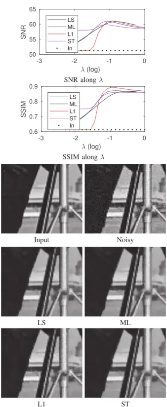
The following Figure 1 shows the performance of the differ-ent methods in terms of SNR and SSIM, for the input image Cameramanas a function of the regularization parameter λ. The parameters used for this simulation are τ = 40 and σ = 10, which produces 7.4% of real outliers in the noisy compressed image. We check that each method achieves an optimal denoising for a given value of λ. Interestingly, the optimal SNR (and thus the mean squared error) is comparable for the three methods ML, LS and L1, while the ST data fit exhibits a lower SNR. In terms of SSIM, the L1 data fit seems to outperform the other methods. Note the specificity of ST, for which even a small value ofλ leads to an acceptable result, since even with a very low regularization the soft-thresholding data-fit manages to dequantize the image.
A zoom of the corresponding denoised images is also displayed on Figure 1, where the optimalλ (in SSIM) has been selected for each method. We clearly see on the noisy images some compression artifacts, caused by both the quantization (near the edges) and the noise (inside the smooth areas). Visually the methods LS, ML and ST seem to give satisfactory results; L1 instead removes most of the outliers caused by the noise but not the compression artifacts near the edges, which is not visually satisfactory.
The results of other simulations on the input images Cam-eraman, Barbara, Lena and Boats are given in Table I. In terms of SSIM, the results are always better for ML (which is very close to LS) when the noise is low; but for higher noise levels corresponding to about 7% of outliers, L1 seems to give the best results.
B. DCT-based compression
We now simulate noisy compressed images obtained with the JPEG compression standard, i.e., when W is the block-DCT. The quantization table for each 8× 8 block is twice the usual one described in [23], and we chooseσ = 8 which produces 7.4% of outliers. The results shown in Figure 2 are comparable with the wavelet (JPEG2000) setting, except that
σ Outliers In LS ML L1 ST Lena 1.31% 0.85 0.87 0.87 0.86 0.86 6 Barb 2.94% 0.85 0.87 0.87 0.86 0.83 Cam 1.20% 0.89 0.91 0.91 0.90 0.90 Boats 1.48% 0.88 0.90 0.90 0.89 0.89 Lena 6.66% 0.58 0.81 0.81 0.84 0.81 12 Barb 9.29% 0.65 0.78 0.78 0.81 0.76 Cam 6.11% 0.57 0.86 0.85 0.88 0.85 Boats 6.58% 0.60 0.84 0.84 0.86 0.83
-3 -2 -1 0 (log) 50 55 60 65 SNR LS ML L1 ST In SNR alongλ -3 -2 -1 0 (log) 0.6 0.7 0.8 0.9 SSIM LS ML L1 ST In SSIM alongλ Input Noisy LS ML L1 ST
Figure 1: JPEG2000 simulations on the Cameraman image.
the LS data fit is in this case clearly outperformed by ML and ST. Again, the L1 loss function effectively removes the “outliers”, i.e., the artifacts caused by the noise, but seems to be less effective for reducing the compression artefacts around the edges of the image.
-3 -2 -1 0 (log) 55 60 65 70 SNR LS ML L1 ST In SNR alongλ -3 -2 -1 0 (log) 0.8 0.85 0.9 0.95 SSIM LS ML L1 ST In SSIM along λ Input Noisy LS ML L1 ST
Figure 2: JPEG simulations on the Cameraman image.
VI. CONCLUSION
This paper presented a generic variational formulation for denoising quantized or compressed images. We introduced two new data-fidelity terms accounting for the transform and quantization used during compression. The two methods
were compared with more standard techniques on numerical experiments in the JPEG and JPEG2000 setting.
When the compression rate is strong whith respect to the noise level (few outliers), which corresponds to the setting encountered in satellite image on-board compression, the two introduced loss functions seem to produce better results than the least-square or the L1 data-fidelity terms, both quantita-tively and visually.
Future works should extend those findings by consider-ing larger image datasets, and more efficient regularizations. Besides, it would be of interest to investigate whether the observed differences bewteen the loss functions still hold when one considers different statistical estimators, e.g., the minimum mean square error (MMSE) estimator instead of the MAP.
ACKNOWLEDGMENTS
This work has been supported by Labex CIMI and by the DEEL program on Dependable and Explainable Learning (www.deel.ai).
REFERENCES
[1] K. Dabov, A. Foi, V. Katkovnik, and K. Egiazarian, “Image denoising by sparse 3-D transform-domain collaborative filtering,” IEEE Transactions on image processing, vol. 16, no. 8, pp. 2080–2095, 2007.
[2] M. Lebrun, A. Buades, and J-M. Morel, “A nonlocal Bayesian image denoising algorithm,” SIAM Journal on Imaging Sciences, vol. 6, no. 3, pp. 1665–1688, 2013.
[3] M. Nikolova, “Minimizers of cost-functions involving nonsmooth data-fidelity terms. Application to the processing of outliers,” SIAM Journal on Numerical Analysis, vol. 40, no. 3, pp. 965–994, 2002.
[4] H. Fu, M. K. Ng, M. Nikolova, and J. L. Barlow, “Efficient minimization methods of mixed l2-l1 and l1-l1 norms for image restoration,” SIAM Journal on Scientific computing, vol. 27, no. 6, pp. 1881–1902, 2006. [5] Y. Traonmilin, S. Ladjal, and A. Almansa, “Robust multi-image
processing with optimal sparse regularization,” Journal of Mathematical Imaging and Vision, vol. 51, no. 3, pp. 413–429, 2015.
[6] M. Lebrun, M. Colom, and J-M. Morel, “The noise clinic: A universal blind denoising algorithm,” in IEEE International Conference on Image Processing (ICIP), 2014, pp. 2674–2678.
[7] R. R. Coifman and A. Sowa, “Combining the calculus of variations and wavelets for image enhancement,” Applied and Computational Harmonic Analysis, vol. 9, no. 1, pp. 1–18, 2000.
[8] F. Alter, S. Durand, and J. Froment, “Adapted total variation for artifact free decompression of JPEG images,” Journal of Mathematical Imaging and Vision, vol. 23, no. 2, pp. 199–211, 2005.
[9] H. Chang, M. K. Ng, and T. Zeng, “Reducing artifacts in JPEG decompression via a learned dictionary,” IEEE transactions on signal processing, vol. 62, no. 3, pp. 718–728, 2014.
[10] A. Zymnis, S. Boyd, and E. Candès, “Compressed sensing with quantized measurements,” IEEE Signal Processing Letters, vol. 17, no. 2, pp. 149–152, 2010.
[11] L. Jacques, D. K. Hammond, and J. M. Fadili, “Dequantizing com-pressed sensing: When oversampling and non-Gaussian constraints combine,” IEEE Transactions on Information Theory, vol. 57, no. 1, pp. 559–571, 2011.
[12] L. I. Rudin, S. Osher, and E. Fatemi, “Nonlinear total variation based noise removal algorithms,” Physica D: Nonlinear Phenomena, vol. 60, no. 1, pp. 259–268, 1992.
[13] F. Malgouyres, “Minimizing the total variation under a general convex constraint for image restoration,” IEEE Transactions on Image Process-ing, vol. 11, no. 12, pp. 1450–1456, 2002.
[14] G. Peyré, S. Bougleux, and L. Cohen, “Non-local regularization of inverse problems,” in European Conference on Computer Vision. Springer, 2008, pp. 57–68.
[15] D. Ulyanov, A. Vedaldi, and V. Lempitsky, “Deep image prior,” in Proceedings of the IEEE Conference on Computer Vision and Pattern Recognition, 2018, pp. 9446–9454.
[16] J. Preciozzi, P. Musé, A. Almansa, S. Durand, F. Cabot, Y. Kerr, A. Khazaal, and B. Rougé, “Sparsity-based restoration of SMOS images in the presence of outliers,” in IEEE International Geoscience and Remote Sensing Symposium (IGARSS), 2012, pp. 3501–3504. [17] P. L. Combettes and V. R. Wajs, “Signal recovery by proximal
forward-backward splitting,” Multiscale Modeling & Simulation, vol. 4, no. 4, pp. 1168–1200, 2005.
[18] I. Daubechies, M. Defrise, and C. De Mol, “An iterative threshold-ing algorithm for linear inverse problems with a sparsity constraint,” Communications on pure and applied mathematics, vol. 57, no. 11, pp. 1413–1457, 2004.
[19] A. Beck and M. Teboulle, “A fast iterative shrinkage-thresholding algorithm for linear inverse problems,” SIAM journal on imaging sciences, vol. 2, no. 1, pp. 183–202, 2009.
[20] P. L. Combettes and J-C. Pesquet, “Proximal splitting methods in signal processing,” in Fixed-point algorithms for inverse problems in science and engineering, pp. 185–212. Springer, 2011.
[21] Z. Wang, A. C. Bovik, H. R. Sheikh, and E. P. Simoncelli, “Image quality assessment: from error visibility to structural similarity,” IEEE transactions on Image Processing, vol. 13, no. 4, pp. 600–612, 2004. [22] P-S. Yeh, P. Armbruster, A. Kiely, B. Masschelein, G. Moury, C.
Schae-fer, and C. Thiebaut, “The new CCSDS image compression recommen-dation,” in IEEE Aerospace Conference, 2005, pp. 4138–4145. [23] G. K. Wallace, “The JPEG still picture compression standard,” IEEE