Codesign mechanics / attitude control for a simplified AOCS preliminary synthesis

To cite this document: Cumer, Christelle and Alazard, Daniel and Grynadier, Alain and

Pittet, Christelle Codesign mechanics / attitude control for a simplified AOCS

preliminary synthesis. (2014) In: ESA GNC 2014 - 9th International ESA Conference on

Guidance, navigation & Control Systems, 2 June 2014 - 6 June 2014 (Porto, Portugal).

O

pen

A

rchive

T

oulouse

A

rchive

O

uverte (

OATAO

)

OATAO is an open access repository that collects the work of Toulouse researchers and

makes it freely available over the web where possible.

This is an author-deposited version published in:

http://oatao.univ-toulouse.fr/

Eprints ID: 13643

Any correspondence concerning this service should be sent to the repository

administrator:

staff-oatao@inp-toulouse.fr

Page 1 of 9

Codesign mechanics / attitude control

for a simplified AOCS preliminary synthesis

Ch. Cumer1, D. Alazard2, A. Grynagier3, Ch. Pittet-Mechin4.

1

ONERA/Systems Control and Flight Dynamics Dept.,31055 Toulouse, France.

2

Université de Toulouse, DMIA, ISAE, 31400 Toulouse, France.

3

Thales Alenia Space, AOCS department, 06156 Cannes La Bocca, France

4

CNES, AOCS department, 31401 Toulouse, France.

ABSTRACT

This paper aims to present the advantages of a multibody modeling approach, adapted to all kinds of satellites. This approach gives not only a linearized satellite model at a nominal parametric configuration but also a linearized parameterized model available on a parametric range. Resulting dynamic models are representative of the couplings between different axes and the impact of flexibility. The two contributions of the paper concern the ability of these dynamic models to simulation purposes and the parameterization of the overall satellite model in terms of the inclination of a flexible appendage, useful for a parametric sensitivity study.

1. INTRODUCTION

Achieving as soon as possible mechanical design parameters, coherently chosen according to control capabilities, is a crucial issue during the preliminary design phase of a spacecraft. For instance it is useful to identify quickly which parameters (frequencies or dampings of flexible modes, inertia gaps between satellite axes, sizing of complex joints...) can limit the performance of AOCS (Attitude and Orbit Control Subsystem) or lead to unstability. But common modeling approaches lead to complete nonlinear black-box-type models, whose accuracy is only appropriate to validation of control laws. Relevant mechanical parameters or parametric uncertainties cannot be explicitly isolated in such models, in order to be optimized or constrained.

In this context this paper exploits a suitable generic modeling method which directly gives structured linearized dynamic models of any multi-body flexible satellite. This approach was first explained in [1] where a linear dynamic model of a satellite around a nominal configuration is set up. The key idea consists in using Euler's equations applied to each subsystem, before connecting them to each other. The method has the great advantage to be generic, when all flexible appendages of a satellite are connected to its rigid main body.

This decomposition subsystem per subsystem also leads to linear synthesis models which highlight interesting physical transfer functions for the synthesis step : for example, in [2], constrained performance requirements are fulfilled with structured H controllers performed on such synthesis models. ∞

Moreover such dynamic models analytically express the impact of dimensioning parameters for the attitude control. That is the reason why they can be easily translated into the LFT (Linear Fractional Transformation) framework such that parametric uncertainties can be taken into account. Resulting models are sufficiently accurate, of medium complexity and adapted to robustness analysis tools, as demonstrated in [3].

The satellite benchmark (described in section 2) studied here allows to prove the ability of the resulting models to AOCS validation and simulation purposes. Indeed an one-axis step SADM (Solar Array Driven Mechanism) is connected to the linearized dynamics model : as seen in section 3, all couplings between the flexible modes and varying axes are recovered. Besides in order to optimize both the structure and the performance of the AOCS, the modelling step can be easily adapted to parameterize the overall satellite model in terms of conception parameters, such as the inclination angle of the flexible appendage (section 4)

2. NOTATIONS

The main notations are here listed.

A. MATHEMATICAL NOTATIONS n m× 0 _{: m× zero matrix n} n n I × : n× identity matrix n T . : transpose operator

dt d

: differential operator with respect to the variable t

B. FRAME DEFINITIONS

The application concerns a satellite composed of a rigid central body and a flexible solar array driven by an one-axis step SADM (Solar Array Driven Mechanism) (see Fig. 1). The solar array is tilted with an angle

γ

and there is a pivot joint between the central body and the flexible appendage.

Fig.1: Reference frames of central body, SADM and flexible array.

Three reference frames must be considered, as highlighted in Fig.1 : the main body reference frame

)

,

,

(

_{CB CB CB}

b

x

y

z

R

=

, the appendage reference frame

R

_a

=

(

x

_GS

,

y

_GS

,

z

_GS

)

and the SADM reference frame

)

,

,

(

_{SADM SADM SADM}

SADM

x

y

z

R

=

. The transformation matrix from

R

_SADM to

R

_bis denoted T_SADM→_CB.

B is the center of mass of the main body and P denotes the anchorage point between the appendage and the main body.

C. MATRIX EXPRESSIONS OF VECTORIAL FORMULAS

If

[

u₁,u₂,u₃

]

T and

[

v₁,v₂,v₃

]

T are the coordinate vectors of respectively the two vectors u and v in a specified frame

R

, the cross product u× is written in v

R

as a matrix-vector product

( )

∗u v where the skew-symmetric matrix

( )

∗u associated to the vector u is defined as follows :

( )

− − − = ∗ 0 0 0 1 2 1 3 2 3 u u u u u u u

This notation is useful to express the transport of a dynamic model from one point to another. Indeed the first-order approximation of the vector, composed of the absolute linear acceleration vector of a body at a point A₁

(aA₁) and of the absolute angular velocity vector of the body w.r.t. the inertial frame (ω), can be rewritten in terms of the absolute accelerations vector of the body at another point A₂ thanks to the relation :

∗ = × × × ω τ ω 2 2 1 1 3 3 3 3 2 1 3 3 0 ) ( A A A A a I A A I a (1)

The transport of the forces vector F and of the torques vector T from A to ₁ A uses the same matrix : ₂

= 2 1 2 1 A T A A A T F T F τ (2)

D. LFT NOTIONS

A linear system submitted to parametric uncertainties can be described by a LFT (Linear Fractional Transformation). This representation consists in isolating the uncertainty matrix ∆ from the nominal model

) (s

H and in connecting them through a feedback as shown in Fig.2. The LFT framework thus allows to represent a continuum of models and over all, avoids launching the modeling procedure again for a new parametric configuration. This is the reason why a LFT model saves CPU time during control attitude validation process, as explained in part 4.

Fig.2: A common LFT model.

3. LINEAR MULTIBODY DYNAMICS EQUATIONS

This section explains briefly how to get a dynamical model of the satellite as physical as possible for simulations and robustness. The reader must refer to [1,3] for further details.

A. LINEAR DYNAMIC MODEL OF THE RIGID MAIN BODY

Under assumptions of small displacements, the Newton's second law and the Euler's equations applied to the rigid main body give :

= − − × × × b B b B B b b B a b B ext a b ext a D II I m T T F F ω , 3 3 3 3 3 3 , / , / 0 0 (3) where :

• F_ext

,

T_ext,B are the external forces/torques (at B ) vectors, applied to the main body,

• F_b/a

,

T_b/a,B are the forces/torques (at B ) vectors, applied by the main body to the appendage, • a is the absolute linear acceleration vector of the main body at B , _B

• ω_b is the absolute angular velocity vector of

R

_b w.r.t. the inertial frame, • m is the mass of the main body, _b

• II_b,B is the 3× moment of inertia tensor of the main body at B . 3 Equation (3) is often written in

R

_b.

B. LINEAR DYNAMIC MODEL OF THE APPENDAGE

If the flexible appendage is cantilevered on the main body at the interface point P , the dynamic model of the appendage describes the relationship between the 6 dof acceleration vector of the point P and the 6 dof forces/torques vector applied by the main body to the appendage at point P :

− = + + + = b P T P i i i P b P a P P a b a b a L diag diag L a D T F ω η ω η ω ξ η η ω ) ( ) 2 ( 2 , / / (4) where : • a P

D is the 6× mass/inertia model matrix of the appendage at point P , 6

• L is the _P 6×N matrix of modal participation factors of the N flexible modes of the appendage at point P ,

Equation (4) is often written in

R

_a. Let us note however that, if the appendage is rigid, its modeling is simpler and looks like the one of the main body.

C. CONNECTION OF THE APPENDAGE TO THE MAIN BODY

A cantilevered connection is easily solved by taking into account (4) into (3). Beforehand (4) must be translated from point P to point B by using (1) and (2). Moreover, as (4) is written in

R

_a, the transformation matrix from

R

_a to

R

_b, denoted

T

_ba.must be applied, as represented in Fig.3.

It is straightforward to notice that a Matlab code can be developed to generate automatically dynamic models of many satellites composed of

• either many rigid/flexible appendages, cantilevered on the rigid main body,

• or a main body with a cantilevered appendage, itself composed of a sequence of cantilevered rigid appendages with the last one being rigid or flexible.

Fig.3: Model of the cantilevered connection between the main body and the flexible appendage. A toolbox [4] is available to generate such linear dynamic models.

But as there is a pivot joint between the central body and the flexible appendage, the rotation around the axis SADM

z (see Fig.1) brings an additional constraint : the only torque submitted by the solar array according to the SADM

z -axis is exactly the torque induced by the SADM. If the linear dynamic model of the appendage is written in

R

_SADM

,

it will lead to :

+ = θ ω ω ω SADM SADM SADM SADM SADM SADM SADM R SADM SADM SADM SADM SADM z b y b x b z P y P x P a P m y P a b x P a b z a b y a b x a b a a a s M C T T F F F , , , , , , , , / , , / , / , / , / ) ( (5)

The expression of θ can be deduced from (5). To have a generic Matlab code, the best procedure consists in considering a state space representation

(

A1,B1,C1,D1

)

of

SADM R

s

MPa( ) where x1 denotes the state vector :

m z b y b x b z P y P x P C D a a a D D x D C SADM SADM SADM SADM SADM SADM ) 6 , 6 ( 1 ) 6 , 6 ( :) , 6 ( ) 6 , 6 ( :) , 6 ( 1 , , , , , , 1 1 1 1 1 _{− +} − = ω ω ω θ (6)

The dynamic model of the appendage is thus augmented with a new input Cm and a new output θ. And as shown in Fig.4.

Fig.4: Augmented direct dynamic model of the appendage on a motorized pivot.

The final dynamic model of the overall system (central body + SADM + flexible array) counts~:

• 4 inputs : the 3 axes torques of attitude control and the torque applied by the SADM to the pivot joint, • 4 outputs : the 3 angular accelerations of the central body and the angular acceleration of the pivot

joint.

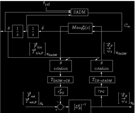
Fig.5 shows how a nonlinear model of SADM can be directly connected to the linear direct dynamic model of the appendage. Frame change (

T

_CB→SADM in Fig.5) allows to restore correctly the dynamic couplings between main body and appendage for each satellite configuration.

Fig. 5: Complete dynamic model of the satellite.

D. SIMULATION OF THE OVERALL SATELLITE SYSTEM

4. COMPUTATION OF A CONTINUUM OF PARAMETERIZED SATELLITE MODELS A. LFT FRAMEWORK FOR PARAMETERIZED SATELLITE MODELS

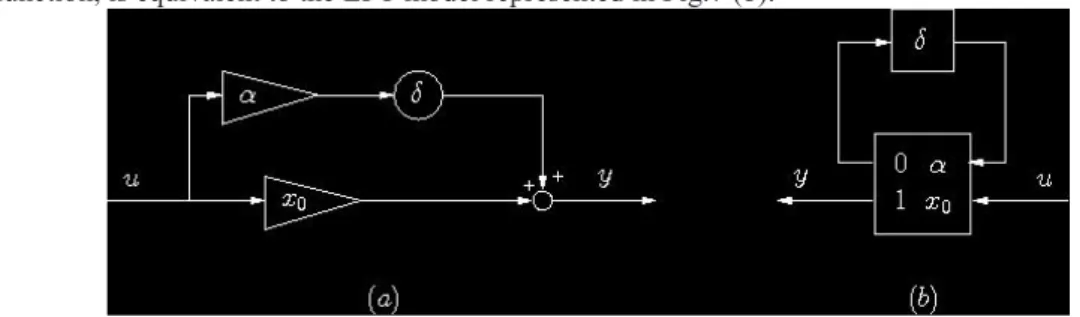
When a parameter whose nominal value is x0 is submitted to uncertainties, two kinds of description are

available :

• either y=(x₀+αδ)u. This is the "additive formulation" and the parameter value is then between α

−

0

x and x₀+α . The block-diagram in Fig.7 (a), which describes the uncertain static transfer function, is equivalent to the LFT model represented in Fig.7 (b).

Fig. 7: Block-diagram in (a) and a LFT in (b) of y=(x₀+αδ)u

.

• or y=x₀(1+αδ)u. It is the so called "multiplicative formulation". The parameter value is then between x₀(1−α) and x₀(1+α). As above, it can be proved that a LFT model exactly describes this new uncertain static transfer function.

These elementary blocks are the basis of the construction of the uncertain complete satellite model. Indeed each uncertain parameter is defined by a characterizing relation (either additive or multiplicative formulation) thanks to a Matlab object (the standard uss in Matlab, or lfr in the LFR Toolbox [5]). This Matlab object can be used as the Matlab object ss : that is the reason why all connections (series, parallel, feedback…) systematically become a LFT model.

As a result, each sub-block in Fig.5 becomes a LFT, depending on the possible parametric uncertainties. The obtained overall linearized dynamic model is finally a LFT model, containing all necessary information to generate all satellite configurations inside the definition range of the uncertain parameters (masses, inertia terms, pulsations and demping ratios of the flexible modes, position of the anchorage points…).

This continuum of parameterized satellite models are useful because it avoids computing the new resulting linear dynamic model when parameter values must be changed.

B. PARTICULAR CASE OF THE INCLINATION ANGLE

This satellite configuration can also be parameterized according to the inclination angle γ (see Fig.1) between the rotation axis of the SADM and the surface of the solar array. Indeed it can be interesting to analyze the impact of this angle value, when the solar array is excited by a step motor. Moreover the obtained LFT model can be parameterized according to the rotation angle θ of the flexible appendage and can be used to validate an attitude control system over a complete revolution of the appendage. To avoid computing models for each γ (or θ) value, the trick consists in isolating, through a feedback, a parameter that allows to generate all models over a γ variation range (or during a complete appendage revolution), so does the LFT building step.

Only a parameterization according to γ will be here detailed.

Let us recall that the angle γ appears in the computation of the matrix Mauga_P(s) (see Fig.1). More precisely the transformation matrix from

R

_SADM to

R

_a can be written as follows :

− = → 0 cos sin 1 0 0 0 sin cos γ γ γ γ a SADM T (7)

If the value of the inclination angle γ can be between 0 deg and γ_MAX deg, this γ range can be described with a normalized uncertainty δγ :

γ δ γ γ γ = ₀+ ₁ with 2 1 0 MAX γ γ γ = = and δ_γ ∈

[

−1,1

]

(8) The matrix raises problems for the LFT building, because it is composed of trigonometric functions, which must verify, whatever the uncertainty value :

(

)

sin

(

)

1

cos2γ0+γ1δγ + 2γ0+γ1δγ =

As a complete revolution is not considered here, a solution, combining ease of the LFT building and size minimization of the uncertainty block, consists in taking the tangent of the half angle. Mathematically,,the notation − ∈ = 2 , 2 2 tan γ1δγ γ1 γ1 t leads to :

(

)

2 1 1 2 1 cos t + + − = δγ γ and

(

)

2 1 1 2 sin t t + = δγ γ

If

[

u₁;u₂;u₃

]

and

[

y₁;y₂;y₃

]

denote respectively the inputs and the outputs of

T

_SADM→a, it is easily to prove that :

(

0 1 0 2

)

₂

(

0 1 0 2

)

2 2 1 sin cos 1 2 sin cos 1 1 u u t t u u t t y γ γ γ + γ + + + − + − =

This equation is represented in Fig.8.

Fig. 8: Block-diagram of the transfer between u₁,u₂and y₁.

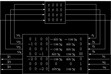
Same developments can be carried on for the expression of y . Fig.9 finally gives a minimal LFT realization of ₃ the matrix

T

_SADM→a

.

Fig. 9: LFT realization of the matrix

T

_SADM→a

.

Let us note that a variable change can normalize the uncertainty : instead of considering t , it is better to work with t~ defined by : t t ~ 2 tan 1 = γ with ~t ∈

[

−1,1

]

.

As explained before this LFT modelling is a CPU time saving procedure, when the best compromise between the definition of the satellite structure and the AOCS performance must be fulfilled.

E. CONCLUSION

This paper proposes an adapted linear modelling procedure for representativeness of the satellite dynamics for AOCS design, for simulation purposes and for all kinds of preliminary steps –namely, the codesign mechanics/attitude control and the robustness analysis of first AOCS. The two main advantages of this method is the genericity of physical models and the simplicity of physical parameter dependence. Extensions are today studied, so that many flexible subsystems can be connected together. This generalization will be useful for in orbit services.

REFERENCES

[1] D. Alazard, Ch. Cumer and K.H.M. Tantawi, “Linear Dynamic Modeling of Spacecraft with Various Flexible Appendages and On-board Angular Momentum”, 7th International ESA Conference on Guidance, Navigation & Control Systems, June 2008, Tralee, Ireland.

[2] N. Guy, D. Alazard, Ch. Cumer, C. Charbonnel, "Reduced order Hinfinity controller synthesis for flexible structures control", IFAC ROCOND, 2012, Aalborg, Denmark.

[3] N. Guy, D. Alazard, C. Cumer, C. Charbonnel, "Dynamic modelling and analysis of spacecraft with variable tilt of flexible appendages", ASME Journal of Dynamic Systems, Measurement and Control, Vol. 136(2), 2014.

[4] Satellite Dynamics Toolbox, Version V1.2, http://personnel.isae.fr/daniel-alazard/matlab-packages/satellite-dynamics-toolbox.html