Open Archive TOULOUSE Archive Ouverte (OATAO)
OATAO is an open access repository that collects the work of Toulouse researchers and
makes it freely available over the web where possible.
This is an author-deposited version published in :
http://oatao.univ-toulouse.fr/
Eprints ID : 15180
The contribution was presented at ECAI 2014),:
http://www.ecai2014.org/
To cite this version :
Bounhas, Myriam and Prade, Henri and Richard, Gilles
Analogical classification: A new way to deal with examples. (2014) In: 21st
European Conference on Artificial Intelligence (ECAI 2014), 18 August 2014 -
22 August 2014 (Pragues, Czech Republic).
Any correspondence concerning this service should be sent to the repository
administrator:
[email protected]
Analogical classification:
A new way to deal with examples
Myriam Bounhas
1and Henri Prade
2and Gilles Richard
3Abstract. Introduced a few years ago, analogy-based classification methods are a noticeable addition to the set of lazy learning tech-niques. They provide amazing results (in terms of accuracy) on many classical datasets. They look for all triples of examples in the train-ing set that are in analogical proportion with the item to be classified on a maximal number of attributes and for which the corresponding analogical proportion equation on the class has a solution. In this pa-per when classifying a new item, we demonstrate a new approach where we focus on a small part of the triples available. To restrict the scope of the search, we first look for examples that are as similar as possible to the new item to be classified. We then only consider the pairs of examples presenting the same dissimilarity as between the new item and one of its closest neighbors. Thus we implicitly build triples that are in analogical proportion on all attributes with the new item. Then the classification is made on the basis of a majority vote on the pairs leading to a solvable class equation. This new algorithm provides results as good as other analogical classifiers with a lower average complexity.
1
Introduction
It is a common sense idea that human learning is a matter of observa-tion, then of imitation and appropriate transposition of what has been observed [1]. This may be related to analogical reasoning [7, 9]. It has been shown that a similar idea can be successful for solving pro-gressive Raven matrices IQ tests, where we build the solution (rather than choosing it in a set of candidates) by recopying appropriate ob-servations [5]. This process is closely related to the idea of analogical proportion, which is a core notion in analogical reasoning [20].
Analogical proportions are statements of the form “A is to B as C is to D”, often denoted A : B :: C : D that express that “A differs fromB as C differs from D”, as well as “B differs from A asD differs from C” [15]. In other words, the pair (A, B) is anal-ogous to the pair(C, D) [6]. A formalized view of analogical pro-portions has been recently developed in algebraic or logical settings [11, 23, 15, 17]. Analogical proportions turn out to be a powerful tool in morphological linguistic analysis [10], as well as in classification tasks where results competitive with the ones of classical machine learning methods have been first obtained by [14].
In classification, we assume here that objects or situations A, B, C, D are represented by vectors of attribute values, denoted ~a,~b, ~c, ~d. The analogical proportion-based approach to classification
1 LARODEC Laboratory, ISG de Tunis, Tunisia & Emirates
Col-lege of Technology, Abu Dhabi, United Arab Emirates, email: myriam−[email protected]
2IRIT, University of Toulouse, France, & QCIS, University of Technology,
Sydney, Australia, email: [email protected]
3IRIT, University of Toulouse, France, email: [email protected]
relies on the idea that the unknown classx = cl( ~d) of a new instance ~
d may be predicted as the solution of an equation expressing that the analogical proportioncl(~a) : cl(~b) :: cl(~c) : x holds between the classes. This is done on the basis of triples(~a,~b, ~c) of examples of the training set that are such that the analogical proportion~a : ~b :: ~c : ~d holds componentwise for all (or on a large number of) the attributes describing the items.
Building the solution of an IQ test or classifying a new item are tasks quite similar. Indeed, the images in a visual IQ test can be de-scribed in terms of features by means of vectors of their correspond-ing values, and we have to find another image represented in the same way, based on the implicit assumption that this latter image should be associated with the given images, this association being governed by the spatial disposition of images in rows, and maybe in columns. Similarly in a classification task, description vectors are associated with classes in the set of examples, while a class has to be predicted for a new vector. In this paper, this parallel leads us to propose a new, more simple and understandable approach to analogy-based classi-fication, inspired from our approach for solving progressive Raven matrices tests [5]. This contrasts with the previous analogical ap-proaches to classification, where all the triples of examples making an analogical proportion with the new item to be classified were con-sidered in a brute-force, blind and systematic manner.
The paper is organized as follows. First, a refresher on analogi-cal proportions both for Boolean and discrete attributes is given in Section 2. Then, in Section 3, a parallel is made between solving IQ tests and classification, where the relevance of analogical propor-tions for analyzing a set of examples is emphasized. After recalling the existing approaches to analogical proportion-based classification in Section 4, the new approach is presented in Section 5, and results on classical benchmarks are reported in Section 6, together with a general discussion on the merits of the new classifier, which may be related to a new learning paradigm that may be called creative
ma-chine learning. Conclusion emphasizes lines for further research.
2
Analogical proportion: a brief background
At the origin of analogical proportion is the standard numerical pro-portion, which is an equality statement between 2 ratios a
b = c d,
wherea, b, c, d are numbers. In the same spirit, an analogical pro-portiona : b :: c : d stating “a is to b as c is to d”, informally expresses that “a differs from b as c differs from d” and vice versa.
As it is the case for numerical proportions, this “analogical” state-ment is supposed to still hold when the pairs(a, b) and (c, d) are exchanged, or when the mean termsb and c are permuted (see [18] for a detailed discussion). When considering Boolean values (i.e. be-longing to B = {0, 1}), a simple way to abstract the symbolic coun-terpart of numerical proportion has been given in [17] by focusing
on indicators to capture the ideas of “similarity” and “dissimilarity”. For a pair(a, b) of Boolean variables, indicators are defined as:
a ∧ b and ¬a ∧ ¬b : similarity indicators, a ∧ ¬b and ¬a ∧ b : dissimilarity indicators.
A logical proportion (see [19] for a thorough investigation) is a con-junction of two equivalences between indicators and the best “clone” of the numerical proportion is the analogical proportion defined as:
(a ∧ ¬b ≡ c ∧ ¬d) ∧ (¬a ∧ b ≡ ¬c ∧ d).
This expression of analogical proportion, using only dissimilarities, could be informally read as what is true fora and not for b is exactly
what is true forc and not for d, and vice versa. As such, a logical proportion is a Boolean formula involving 4 variables and it can be checked on Table 1 that the logical expression ofa : b :: c : d satisfies symmetry (a : b :: c : d → c : d :: a : b) and central
permutation(a : b :: c : d → a : c :: b : d), which are key properties of an analogical proportion acknowledged for a long time. Moreover, this Boolean modeling still enjoys the transitivity property (a : b :: c : d) ∧ (c : d :: e : f ) → (a : b :: e : f ). a b c d a: b :: c : d 0 0 0 0 1 1 1 1 1 1 0 0 1 1 1 1 1 0 0 1 0 1 0 1 1 1 0 1 0 1
Table 1. Valuations wherea : b :: c : d is true
In terms of generic patterns, we see that analogical proportion always holds for the 3 following patterns:s : s :: s : s, s : s :: t : t and s : t :: s : t where s and t are distinct Boolean values.
One of the side products of numerical proportions is the well-known “rule of three” allowing to compute a suitable 4th itemx in order to complete a proportion a
b = c
x. This property has a
counter-part in the Boolean case where the problem can be stated as follows. Given a triple(a, b, c) of Boolean values, does there exist a Boolean valuex such that a : b :: c : x = 1, and in that case, is this value unique? There are cases where the equation has no solution since the triple(a, b, c) may take 23= 8 values, while a : b :: c : d is true only
for 6 distinct 4-tuples. Indeed, the equations1 : 0 :: 0 : x = 1 and 0 : 1 :: 1 : x = 1 have no solution. It is easy to prove that the analog-ical equationa : b :: c : x = 1 is solvable iff (a ≡ b)∨(a ≡ c) holds true. In that case, the unique solution is given byx = a ≡ (b ≡ c).
Back to our 3 analogical patternss : s :: s : s, s : s :: t : t and s : t :: s : t, solving an incomplete pattern (i.e. where the 4th element is missing) is just a matter of copying a previously seen values or t (an idea already emphasized in [5]).
Objects are generally represented as vectors of attribute values (rather than by a single value). Here each vector component is as-sumed to be a Boolean value. A straightforward extension to Bnis:
~a : ~b :: ~c : ~d iff ∀i ∈ [1, n], ai: bi:: ci: di
All the basic properties (symmetry, central permutation) still hold for vectors. The equation solving process is also valid, but provides a new insight about analogical proportion: analogical proportions are creative. Indeed let us consider the following example where ~a = (1, 0, 0),~b = (0, 1, 0) and ~c = (1, 0, 1). Solving the analogical equation~a : ~b :: ~c : ~x yields ~x = (0, 1, 1), which is a vector different from~a,~b and ~c. In fact, we can extend this machinery from Boolean to discrete domains where the number of candidate attribute values is finite, but greater than 2. Indeed, considering an attribute domain {v1, · · · , vm}, we can binarize it by means of the m properties
“hav-ing or not valuevi”. For instance, given a tri-valued attribute having
candidate valuesv1, v2, v3, respectively encoded as100, 010, 001,
the valid analogical proportion v1 : v2 : v1 : v2 still holds
com-ponentwise as a B3 vector proportion:100 : 010 :: 100 : 010, since the Boolean proportions1010, 0101 and 0000 hold. It can be checked that the binary encoding acknowledges the analogical pro-portions underlying the two other patternsv1 : v1 : v2 : v2 and
v1 : v1 : v1 : v1as well. Conversely, a non-valid analogical
pro-portion, e.g.v1 : v2 : v2 : v1, will not be recognized as an
ana-logical proportion in this binary encoding. This remark will enable us to handle discrete attributes directly in terms of the three patterns s : s :: s : s, s : s :: t : t and s : t :: s : t, where s and t are now values of a discrete attribute domain4.
3
From IQ tests to analogical classifiers
A training setT S of examples ~xk= (xk
1, ..., xki, ..., xkn) together
with their classcl( ~xk), with k = 1, · · · , t can receive an informal
reading in terms of analogical proportions. Namely, “ ~x1is tocl( ~x1)
as ~x2is tocl( ~x2) as · · · as ~xtis tocl( ~xt)” (still assuming transitivity
of these analogical proportions). This can be (informally) written as ~
x1: cl( ~x1) :: ~x2: cl( ~x2) :: · · · :: ~xt: cl( ~xt)
It is important to notice that this view exactly fits with the idea that in a classification problem there exists an unknown classification
func-tionthat associates a unique class with each object, and which is exemplified by the training set. Indeed ~xk : cl( ~xk) :: ~xk : cl′
( ~xk)
withcl( ~xk) )= cl′( ~xk) is forbidden, since it cannot hold as an
ana-logical proportion. However in practice, we allow noise inT S, i.e. examples ~xkwith a wrong classcl( ~xk). The training set is not just
viewed as a simple set of pairs(~x, cl(~x)), but as a set of valid ana-logical proportions~x : cl(~x) :: ~y : cl(~y). This is the corner stone of the approach presented in the following.
A similar view has been recently successfully applied to the solv-ing of Raven progressive matrix IQ tests [5]. In this type of tests you have to complete a3 × 3 matrix where the contents of the 9th case is missing. Then the starting point of the approach was to assume that
(cell(1, 1), cell(1, 2)) : cell(1, 3) :: (cell(2, 1), cell(2, 2)) : cell(2, 3) ::
(cell(3, 1), cell(3, 2)) : cell(3, 3)
wherecell(i, j) is a multiple-attribute, vector-based representation of the contents of the cell(i, j), cell(3, 3) being unknown. The above formal expression states that the pair of the first two cells of line 1 is to the third cell of line 1 as the pair of the first two cells of line 2 is to the third cell of line 2, as the pair of the first two cells of line 3 is to the third cell of line 3 (similar analogical proportions are also assumed for columns). Here the hidden functionf is such that cell(i, 3) = f (cell(i, 1), cell(i, 2)), and its output is not a class, but a cell description. Since this approach has been successful for solving Raven IQ tests, the idea in this paper is to apply it to classification.
Applying central permutation, we are led to rewrite the analogical proportion ~xi: cl( ~xi) :: ~xj: cl( ~xj) linking examples ~xiand ~xjas
~
xi: ~xj:: cl( ~xi) : cl( ~xj)
This suggests a new reading of the training set, based on pairs. Namely, the ways vectors ~xiand ~xjare similar / dissimilar should be
related to the identity or the difference of classescl( ~xi) and cl( ~xj).
Given a pair of vectors ~xi and ~xj, one can compute the set of at-4 However, note that some proportions may be known to hold between
at-tribute values (e.g. “small : medium :: medium : large”), while they do not match any of the 3 patterns, and as such will not be recognized.
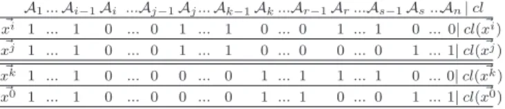
A1...Ai−1Ai ...Aj−1Aj...Ak−1Ak...Ar−1Ar...As−1As...An| cl # xi 1 ... 1 0 ... 0 1 ... 1 0 ... 0 1 ... 1 0 ... 0| cl(x#i) # xj 1 ... 1 0 ... 0 1 ... 1 0 ... 0 0 ... 0 1 ... 1| cl(x#j) # xk 1 ... 1 0 ... 0 0 ... 0 1 ... 1 1 ... 1 0 ... 0| cl(x#k) # x0 1 ... 1 0 ... 0 0 ... 0 1 ... 1 0 ... 0 1 ... 1| cl(x#0) Table 2. Pairing two pairs
tributesA( ~xi, ~xj) where they agree (i.e. they have identical attribute
values) and the set of attributesD( ~xi, ~xj) where they disagree (i.e.
they have different attribute values). Thus, in Table 2, after a suitable reordering of the attributes, the vectors ~xiand ~xjagree on attributes
A1toAr−1and disagree on attributesArtoAn. Consider now the
instance ~x0 (see Table 2) for which we want to predict the class.
Suppose, we have in the training setT S, both the pair ( ~xi, ~xj), and
the example ~xkwhich once paired with ~x0has exactly the same
dis-agreement setasD( ~xi, ~xj) and moreover with the changes oriented
in the same way. Then, as can be seen in Table 2, we have a per-fect analogical proportion componentwise, between the four vectors. Note that althoughA( ~xi, ~xj) = A( ~xk, ~x0), the four vectors are not
everywhere equal on this subset of attributes. Besides, note also that the above view would straightforwardly extend from binary-valued attributes to attributes with finite attribute domains.
Thus, working in this way with pairs, we can implicitly reconsti-tute 4-tuples of vectors that form an analogical proportion as in the triple-based brute force method approach to classification. Before de-veloping this pair-based approach from an algorithmic point of view, let us first recall the previously existing approaches that are based on the systematic use of triples of examples.
4
Triples-based analogical classifiers
Numerical proportions are closely related to the ideas of extrapola-tion and of linear regression, i.e., to the idea of predicting a new value on the ground of existing values. The equation solving property re-called above is at the root of a brute force method for classification. It is based on a kind of proportional continuity principle: if the binary-valued attributes of 4 objects are componentwise in analogical pro-portion, then this should still be the case for their classes. More pre-cisely, having a binary classification problem, and 4 Boolean objects ~a,~b, ~c, ~d, 3 in the training set with known classes cl(~a), cl(~b), cl(~c), the 4th being the object to be classified in one of the classes, i.e.cl( ~d) is unknown, this principle can be stated as:
~a : ~b :: ~c : ~d cl(~a) : cl(~b) :: cl(~c) : cl( ~d)
Then, if the equationcl(~a) : cl(~b) :: cl(~c) : x is solvable, we can allocate its solution tocl( ~d). Note that this applies both in the case where attributes and classes are Boolean and in the case where at-tribute values and classes belong to discrete domains. This principle can lead to several implementations (in the Boolean case).
Before introducing the existing analogical classifiers, let us first restate the classification problem. We consider a universe U where each object is represented as a vector of n feature val-ues ~x = (x1, ..., xi, ..., xn) belonging to a Cartesian product
T = Πi∈[1,n]Xi. When considering only binary attributes, it simply
meansT = Bn
. Each vector~x is assumed to be part of a group of vectors labeled with a unique classcl(~x) ∈ C = {c1, ..., cK}, where
K is finite and there is no empty class in the data set. If we suppose thatcl is known on a subset T S ⊂ T (T S is the training set or the example set), given a new vector~y = (y1, ..., yi, ..., yn) /∈ T S, the
classification problem amounts to assigning a plausible valuecl(~y) on the basis of the examples stored inT S.
Learning by analogy as described in [2], is a lazy learning tech-nique which uses a measure of analogical dissimilarity between 4 objects. It estimates how far 4 objects are from being in ana-logical proportion. Roughly speaking, the anaana-logical dissimilarity adbetween 4 Boolean values is the minimum number of bits that have to be switched to get a proper analogy. Thus ad(1, 0, 1, 0) = 0, ad(1, 0, 1, 1) = 1 and ad(1, 0, 0, 1) = 2. Thus, a : b :: c : d holds if and only if ad(a, b, c, d) = 0. Moreover ad differentiates two cases where analogy does not hold, namely the 8 cases with an odd number of 0 and an odd number of 1 among the 4 Boolean val-ues, such as ad(0, 0, 0, 1) = 1 or ad(0, 1, 1, 1) = 1, and the two cases ad(0, 1, 1, 0) = ad(1, 0, 0, 1) = 2. When we deal with 4 Boolean vectors in Bn, adding the ad evaluations componentwise generalizes the analogical dissimilarity to Boolean vectors, and leads to an integer AD belonging to the interval[0, 2n]. This number es-timates how far the 4 vectors are from building, componentwise, a complete analogy. It is used in [2] in the implementation of a classi-fication algorithm where the input parameters are a setT S of classi-fied items, an integerk, and a new item ~d to be classified. It proceeds as follows:
Step 1: Compute the analogical dissimilarity AD between ~d and all the triples inT S3that produce a solution for the class of ~d.
Step 2: Sort thesen triples by the increasing value of AD. Step 3: Letp be the value of ad for the k-th triple, then find k′
as being the greatest integer such that thek′
-th triple has the valuep. Step 4: Solve thek′
analogical equations on the label of the class. Take the winner of thek′
votes and allocate this winner tocl( ~d). This approach provides remarkable results and, in several cases, outperforms the best known algorithms [14]. Other options are avail-able that do not use a dissimilarity measure but just apply in a straightforward manner the previous continuity principle, still adding flexibility by allowing to have some components where analogy does not hold. A first option [17, 21] is to consider triples(~a,~b, ~c) such that the class equationcl(~a) : cl(~b) :: cl(~c) : x is solvable and such thatcard({i ∈ [1, n]| ai : bi :: ci : diholds}) is
maxi-mal. Then we allocate to ~d the label solution of the corresponding class equation. A second option [16] is to fix an integerp telling us for how many components we tolerate the analogical proportion not to hold. In that case, a candidate voter is just a triple(~a,~b, ~c) such that the class equationcl(~a) : cl(~b) :: cl(~c) : x is solvable and card({i ∈ [1, n]| ai: bi:: ci: diholds} ≥ n − p). In both options
[21, 16], a majority vote is applied among the candidate voters. The main novelty wrt the previous approach [2] is that we do not differen-tiate the two cases where analogy does not hold. In terms of accuracy there is no significant differences between these three algorithms.
5
A pair-based approach
In this section, we investigate a new approach to analogical classi-fication, simpler that the known ones. The main idea is first to look for the items inT S that are the most similar to the new item ~d to be classified, then to look for pairs inT S2that present the same dissim-ilarity as the one existing between ~d and the chosen nearest neighbor. We thus build triples used for final prediction. Let us detail the idea.
Step 1: Use of similarity.We look for the most similar examples to ~d. Let ~c be a nearest neighbor of ~d in T S. If ~c = ~d, (i.e. ~d belongs toT S), its label is known and there is nothing to do. In the opposite case~c )= ~d, ~c differs from ~d on p values (i.e. the Hamming distance between~c and ~d, H(~c, ~d) equals to p). Since ~c is a nearest neighbor
of ~d w.r.t. H, there is no example ~c′differing from ~d on less than p
values. However, unlike1-nn algorithm, we do not allocate the label of~c to ~d: this is the exact point where analogical learning differs from thek-N N family of algorithms.
Step 2: Use of dissimilarity.Now, we search inT S a pair (~a,~b) of examples dissimilar in the same way as~c and ~d are dissimilar. Moreover~a and ~b should be identical on the same attributes where ~c and ~d are identical. For instance, if ~c = (1, 0, 1, 1, 1, 0), ~d = (0, 1, 1, 0, 1, 0), ~a and ~b should be similar (i.e. identical) on at-tributes 3, 5 and 6 and dissimilar on atat-tributes 1, 2 and 4, ex-actly as ~c and ~d are dissimilar. In that particular case, the pair ~a = (1, 0, 0, 1, 0, 0),~b = (0, 1, 0, 0, 0, 0) satisfies the previous re-quirement. Clearly,~a : ~b :: ~c : ~d is a valid analogical proportion.
In the case where the class equationcl(~a) : cl(~b) :: cl(~c) : x has a solution, we allocate tocl( ~d) the solution of this equation. If not, we search for another pair(~a,~b). Obviously, in the case where we have more than one nearest neighbor~c or several pairs (~a,~b), leading to different labels for ~d, we implement a majority vote for the final label of ~d. In case there are ties, i.e. several classes get the same maximal number of votes, we consider the set of neighbors~c at distance p + 1, and we repeat the same procedure restricted to the subset of winning classes. We iterate the process until having a unique winner.
Let us now state these ideas with formal notations in the Boolean case (the extension to the discrete case is easy). Given 2 distinct vec-tors~x and ~y of Bn
, they define a partition of[1, n] as • A(~x, ~y) = {i ∈ [1, n]| xi= yi} capturing the similarities,
• D(~x, ~y) = {i ∈ [1, n]| xi)= yi} = [1, n] \ A(~x, ~y) capturing the
dissimilarities. The cardinal ofD(~x, ~y) is exactly the Hamming distanceH(~x, ~y) between the 2 vectors.
GivenJ ⊆ [1, n], let us denote ~x|J the subvector of~x made of
thexj,j ∈ J. Obviously, ~x|A(1x,1y) = ~y|A(1x,1y) and, in the binary
case, when we know~x|D(1x,1y), we can compute~y|D(1x,1y). The pair
(~x, ~y) allows us to build up a disagreement pattern Dis(~x, ~y) as a list of pairs (value, index) (value ∈ Bn, index ∈ D(~x, ~y))
where the 2 vectors differ. In the binary case, withn = 6, ~x = (1, 0, 1, 1, 0, 0), ~y = (1, 1, 1, 0, 1, 0), Dis(~x, ~y) = (02, 14, 05). It
is clear that having a disagreement patternDis(~x, ~y) and a vector ~x (resp.~y), we can get ~y (resp. ~x). In the same way, the disagreement patternDis(~y, ~x) is deducible from Dis(~x, ~y). For the previous ex-ample,Dis(~y, ~x) = (12, 04, 15).
The previous explanation can now be described with the pseudo-code of Algorithm 1, where theunique(value, Array) function re-turns a Boolean valuetrue iff the value value appears exactly once in the arrayArray, f alse otherwise.
LetBH( ~d, r) = {~c ∈ T S | H( ~d, ~c) = r} be the ball in T S with
center ~d and radius r w.r.t. the Hamming distance H. The algorithm stops as soon as we have a label for ~d, and we do not investigate other balls with bigger radius where we could find other options. Note that these balls do not overlap by construction. If we do not find any label for ~d, the algorithm stops when r = n + 1 and returns not classif ied. We cannot classify in the case there is a 50/50 vote: from a probability viewpoint, this situation is extremely unlikely and did not happen for the benchmarks we have dealt with.
We have to note that an offline pre-processing can be done on the training setT S: for each r ∈ [1, n], we can build up the subset of T S × T S constituted with the pairs (~a,~b) such that H(~a,~b) = r: this will speed up the online process within the internal FOR loop.
Due to the two nested FOR loops, it is clear that the worse case complexity is cubic (as the other analogy-based algorithms) since
Algorithm 1 Analogical classifier
Input: ~d /∈ T S a new instance to be classified r = 1; classif ied = f alse;
while not(classif ied) AND (r ≤ n) do
build up the setBH( ~d, r) = {~c ∈ T S|H(~c, ~d) = r}
ifBH( ~d, r) )= ∅ then
for each labell do CandidateV ote(l) = 0 end for for each~c in BH( ~d, r) do
for each pair (~a,~b) such that: Dis(~a,~b) = Dis(~c, ~d) AND cl(~a) : cl(~b) :: cl(~c) : x has solution l do
CandidateV ote(l) + + end for
end for
maxi = max{CandidateV ote(l)}
if maxi )= 0 AND unique(maxi, CandidateV ote(l)) then
cl( ~d) = argmaxl{CandidateV ote(l)}
classif ied = true end if
end if r + + end while ifclassif ied then
return (cl( ~d)) else
return (not classif ied)) end if
the search space is justT S × T S × T S. Nevertheless, in average, we will find a solution within the ballBH( ~d, r) with r < n, thus
pruning a large part of the search space. Besides, one may think of the pre-processing step working only on a subset ofT S.
It is important to remark that the cardinality of a Hamming ball depends on the data representation. Let us illustrate the problem with only 2 attributes a1 and a2 where a1 is binary and a2 is
nominal with 3 possible distinct values. Given 2 distinct exam-ples ~d = (1, v1) and ~d′ = (1, v2) respectively represented as
~
d = (1, 1, 0, 0) and ~d′= (1, 0, 1, 0) when binarized. With discrete
coding,H( ~d, ~d′) = 1, i.e. ~d′ ∈ B
H( ~d, 1), but with the binary
cod-ing,H( ~d, ~d′) = H((1, 1, 0, 0), (1, 0, 1, 0)) = 2 i.e. ~d′∈ B/ H( ~d, 1).
Ultimately, the number of voters will not be the same and we can anticipate different results depending on the coding method.
6
Experiments
This section provides experimental results obtained with our new al-gorithm. The experimental study is based on six data sets taken from the U.C.I. machine learning repository [13].
- Balance and Car are multiple classes databases.
- TicTacToe, Monk1, Monk2 and Monk3 data sets are binary class problems. Monk3 has noise added (in the training set only).
A brief description of these data sets is given in Table 3. Table 3. Description of datasets
Datasets Instances Nominal Att. Binary Att. Classes
Balance 625 4 20 3 Car 743 7 21 4 TicTacToe 958 9 27 2 Monk1 432 6 15 2 Monk2 432 6 15 2 Monk3 432 6 15 2
Table 4 provides the accuracy results for the proposed algorithm obtained with a 10-fold cross validation for these six datasets. The best results are highlighted in bold. Several comments arise:
Table 4. Accuracy results (means and standard deviations)
non binarized binarized
r=1 r=2 r=3 r=1 r=2 r=3 Balance 86± 4 88± 2 72± 5 84± 4 87± 3 74± 5 Car 95± 3 89± 3 72± 6 95± 3 94± 5 77± 6 TicTacToe 98± 5 96± 5 98± 5 98± 5 97± 5 98± 5 Monk1 99± 1 99± 1 90± 4 99± 1 99± 1 99± 1 Monk2 99± 1 97± 3 91± 5 60± 7 99± 1 94± 5 Monk3 99± 1 97± 2 91± 5 99± 1 99± 1 98± 2
• In Table 4 it is clear that the results are not code-sensitive (except for Monk2 dataset): whatever the way we code the data, keeping the discrete values or moving to a binary code, we get the same accuracy (the difference is not statistically significant). Regarding the case of Monk2, it is known that the underlying function (“hav-ing exactly two attributes with value 1”) is more complicated than the functions underlying Monk1 and Monk3, and involves all the attributes (while in the two other functions only 3 attributes among 6 are involved). Then we may conjecture that more examples are needed in Monk2 for predicting the function. For Monk2, in the Hamming ball of radius 1, the average number of voters is 220 in the discrete case while it is only 64 in the binarized case which might be not enough to accurately predict this complex function. • Roughly speaking, our best results are obtained for small values
ofr (often the smallest one, r = 1), at least in the discrete case, since in the binary case, we observe on some datasets that a very good accuracy result may be obtained with a higher value ofr in the case of binary coding, which is consistent with the above analysis.
• From a practical perspective, these results suggest that we might consider that the pairs differing on one attribute are sufficient to classify new items ~d and that we have just to explore BH( ~d, 1) for
associating a label to ~d. This rule of thumb will drastically reduce the size of the search space and then the average complexity of the algorithm, but it has to be investigated in a broader experimenta-tion. This value ofr is also likely to be connected with the size of the training set (a too small training set may lead to an empty ball forr = 1).
• Let us also mention that for the 6 considered datasets, we did not get any “not classified items”. This means that in practice, there always exists a ballBH( ~d, r) where a majority vote can take place.
It is interesting to figure out the numbers of pairs (~a,~b) that are built from the training set (in pre-processing step) that differ onr attributes for1 ≤ r ≤ n. Let us consider the case of Monk2 (with a discrete coding), whenT S is equal to 90% of the whole data set. The number of pairs(~a,~b) is:
r = 1 : 3946; r = 2 : 17346; r = 3 : 39630; r = 4 : 49580; r = 5 : 32068; r = 6 : 8362. The sum of these numbers equals the numbers of pairs that can be built from the used part of the data set. As expected, this number first increases withr and then decreases. When considering a particular item ~d, and a neighbor ~c ∈ BH( ~d, r)
the number of voters(~a,~b) is a small subset of the set of pairs dif-fering onr attributes, due to the fact that two constraints have to be satisfied: the pairs(~a,~b) and (~c, ~d) differ on the same attribute(s) and the associated class equation should be solvable. For instance, in the Monk2case (with a discrete coding), forr = 1, the average number of voters is 220, forr = 2, 350, for r = 3, 270. However with the binary coding, forr = 2 and r = 3, the average number of voters would be smaller as it is the case forr = 1.
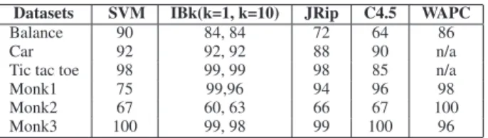
In order to compare analogical classifiers with existing classifica-tion approaches, Table 5 includes classificaclassifica-tion results of some ma-chine learning algorithms: the SVM, k-Nearest Neighbors IBk for k=1, k=10, JRip an optimized propositional rule learner, C4.5 deci-sion tree and finally WAPC, the weighted analogical classifier (us-ing analogical dissimilarity) presented in [14]. Accuracy results for SVM, IBk, JRip and C4.5 are obtained by applying the free imple-mentation of Weka software.
Table 5. Classification results of well-known machine learning algorithms Datasets SVM IBk(k=1, k=10) JRip C4.5 WAPC
Balance 90 84, 84 72 64 86
Car 92 92, 92 88 90 n/a
Tic tac toe 98 99, 99 98 85 n/a
Monk1 75 99,96 94 96 98
Monk2 67 60, 63 66 67 100
Monk3 100 99, 98 99 100 96
We draw the following conclusions from this comparative study: • As expected, our results are very close to, and as good as, those
obtained by the other analogical based-approach WAPC. • However, in contrast with WAPC, we do not use any weighting
machinery for improving the basic algorithm.
• Moreover, let us note that, with our new approach, when we compare with the WAPC algorithm using analogical dissimilarity (AD), we only use candidate voters with AD= 0 (perfect analogy on all attributes). Indeed it has been observed in [14] that the num-ber of triples(~a,~b, ~c) such that AD(~a,~b, ~c, ~d) = 0 is often large. Our results show that it is enough to consider these perfect triples (obtained as the combination of a nearest neighbor~c and of a pair (~a,~b) in the new approach) to make accurate predictions. • As WAPC, the new algorithm provides results which can be
favor-ably compared with classical methods (at least for these datasets), and even sometimes outperforming their results.
When the Hamming distancer is small, which is usually the case, ~a is quite close to ~b, since ~c is close to ~d. Nevertheless, it has been checked that in general this is no longer the case that~a or ~b are close to ~d. This highlights the fact that such classifiers do not work in the neighborhood of the item to be classified but rather look for pieces of information far from the target item ~d.
However, as an attempt to make analogical classifiers closer to k-N k-N classifiers, we also tested another version of the proposed algo-rithm that only considers as candidate voters the pairs(~a,~b) that are equal to the pair(~c, ~d) on the greatest possible number of attributes. Obtained results for the datasets (discrete coding) are as follows: r=1 Monk1: 87±8; Monk2: 64±5; Monk3: 91±6; Balance: 78±5; Car: 88±2.
r=2 Monk1: 88±9; Monk2: 58±7: Monk3: 95±3; Balance: 86±5; Car: 80±6.
From these results compared to those given in Table 4, it is clear that this new version is significantly less accurate than the basic one. We can conclude that considering only pairs(~a,~b) equal to (~c, ~d) for a maximum number of attributes is not very effective for clas-sification. This suggests that, doing this, we remain too close to the spirit ofk-N N classifiers for getting the full benefit of the analogical proportion-based approach.
Lastly, we tested a third version of the proposed approach which is different from the second one. Instead of classifying the example ~
d using the pairs (~a,~b) that are equal to the pair (~c, ~d) on a maxi-mum number of attributes, we classify the example using pairs(~a,~b) which are equal to(~c, ~d) on a chosen number r of attributes. This
numberr is taken as the one for which the number of pairs (~a,~b) is maximum, i.e., r = argmaxr′{card(E(1c,1d)∩ E′ (1c,1d)) | H( ~d, ~c) = r ′ } withE(1c, 1d)= {(~a,~b) ∈ T S
2|Dis(~a,~b) = Dis(~c, ~d)} and
E′
(1c,1d) = {(~a,~b) ∈ T S
2|cl(~a) : cl(~b) :: cl(~c) : x is solvable}
The experiment shows that this version has classification results very close to those given in Table 4 for the basic algorithm.
Thus, in analogical classifiers, contrary tok-N N approaches, we deal with pairs of examples. Moreover, the two pairs that are involved in an analogical proportion are not necessarily much similar as pairs, beyond the fact they should exhibit the same dissimilarity (on a usu-ally small number of attributes). At least from an experimental view-point, this way to proceed appears to be effective enough to get good performances.
Our approach may appear somehow similar to works coming from the CBR community. Nevertheless our method entirely relies on ana-logical proportions involving a triple of examples together with an item to be classified. Instead of considering all candidate triples, we focus on a subset of triples by choosing one of the three elements of the triple as a nearest neighbor of the new item. There is no con-straint on the 2 other elements in the triple which may then be found far from the immediate neighborhood of the item to be classified. We are neither bracketing the item between two examples as in [12], nor using any Bayesian techniques as in [4]. From another viewpoint, adaptation is crucial in the CBR community and adaptation knowl-edge can be learned (see [8] for instance), to be applied to the pairs (new item, a nearest neighbor). In our approach, analogical propor-tions handle similarity and dissimilarity simultaneously, performing a form of adaptation in their own way, without the need for any in-duction step. Finally, it is worth to note that a similar approach for handling numerical attributes has been investigated in [3], also lead-ing to promislead-ing results.
7
Conclusion
In this paper, we have presented a new way to deal with analogi-cal proportions in order to design classifiers. Instead of a brute-force investigation of all the triples~a,~b, ~c to build up a valid proportion with the new item ~d to be classified, we first look for a neighbor ~c of ~d. Then, on the basis of the dissimilarities between ~c and ~d, we find the pairs(~a,~b) with exactly the same dissimilarities. Such pairs, associated with~c constitute the candidate voters provided that the corresponding class equation is solvable. Our first implementation exhibits very good results on 6 UCI benchmarks and enjoys a lower average complexity than classical analogical classifiers. This has to be confirmed on bigger datasets (more attributes, more examples).
As explained in the Monk2 example, a rather small number of pair-based voters are used to classify. It remains to investigate if this is a general property and if it is possible to obtain accurate results by focusing only on a still more restricted number of voters. Such an approach might be closer to a cognitive attitude where excellent human experts usually focus directly on the few relevant pieces of information for making prediction (classification or diagnosis) [22].
Analogical proportions are not only a tool for classifying, but more generally for building up a 4th item starting from 3 others, thanks to the equation solving process. As we have seen, this 4th item could be entirely new. Thus, while classifiers likek-N N focus on the neighborhood of the target item, analogical classifiers go beyond this neighborhood, and rather than “copying” what emerges among close neighbors, “take inspiration” of relevant information possibly far from the immediate neighborhood. Finally, this way to proceed
with analogical proportions is paving the way to what could be called “creative machine learning”.
REFERENCES
[1] A. Bandura, Social Learning Theory, Prentice Hall, 1977.
[2] S. Bayoudh, L. Miclet, and A. Delhay, ‘Learning by analogy: A clas-sification rule for binary and nominal data’, Proc. Inter. Joint Conf. on
Artificial Intelligence IJCAI07, 678–683, (2007).
[3] M. Bounhas, H. Prade, and G. Richard, ‘Analogical classification: Han-dling numerical data’, Technical Report RR–2014-06–FR, Institut de Recherche en Informatique de Toulouse (IRIT), (May 2014). [4] W.w. Cheng and E. H¨ullermeier, ‘Combining instance-based
learn-ing and logistic regression for multilabel classification’, Mach. Learn., 76(2-3), 211–225, (Sep 2009).
[5] W. Correa, H. Prade, and G. Richard, ‘When intelligence is just a matter of copying’, in Proc. 20th Eur. Conf. on Artificial Intelligence,
Mont-pellier, Aug. 27-31, pp. 276–281. IOS Press, (2012).
[6] M. Hesse, ‘On defining analogy’, Proceedings of the Aristotelian
Soci-ety, 60, 79–100, (1959).
[7] K. J. Holyoak and P. Thagard, Mental Leaps: Analogy in Creative
Thought, MIT Press, 1995.
[8] J. Jarmulak, S. Craw, and R. Rowe, ‘Using case-base data to learn adap-tation knowledge for design’, in Proceedings of the 17th International
Joint Conference on Artificial Intelligence - Volume 2, IJCAI’01, pp. 1011–1016, San Francisco, CA, USA, (2001). Morgan Kaufmann Pub-lishers Inc.
[9] S. E. Kuehne, D. Gentner, and K. D. Forbus, ‘Modeling infant learning via symbolic structural alignment’, in Proc. 22nd Annual Meeting of
the Cognitive Science Society, pp. 286–291, (2000).
[10] J. F. Lavall´ee and P. Langlais, ‘Moranapho: un syst`eme multilingue d’analyse morphologique bas´e sur l’analogie formelle’, TAL, 52(2), 17– 44, (2011).
[11] Y. Lepage, ‘Analogy and formal languages’, Electr. Notes Theor.
Com-put. Sci., 53, (2001).
[12] D. McSherry, ‘Case-based reasoning techniques for estimation’, in IEE
Colloquium on Case-Based Reasoning, pp. 6/1–6/4, (Feb 1993). [13] J. Mertz and P.M. Murphy, ‘Uci repository of machine learning
databases’, Available at:
ftp://ftp.ics.uci.edu/pub/machine-learning-databases, (2000).
[14] L. Miclet, S. Bayoudh, and A. Delhay, ‘Analogical dissimilarity: defi-nition, algorithms and two experiments in machine learning’, JAIR, 32, 793–824, (2008).
[15] L. Miclet and H. Prade, ‘Handling analogical proportions in classi-cal logic and fuzzy logics settings’, in Proc. 10th Eur. Conf. on
Sym-bolic and Quantitative Approaches to Reasoning with Uncertainty (EC-SQARU’09),Verona, pp. 638–650. Springer, LNCS 5590, (2009). [16] R. M. Moraes, L. S. Machado, H. Prade, and G. Richard, ‘Classification
based on homogeneous logical proportions’, in Proc. of AI-2013, The
Thirty-third SGAI International Conference on Innovative Techniques and Applications of Artificial Intelligence, Cambridge, England, UK,, eds., M. Bramer and M. Petridis, pp. 53–60. Springer, (2013). [17] H. Prade and G. Richard, ‘Reasoning with logical proportions’, in Proc.
12th Int. Conf. on Principles of Knowledge Representation and Rea-soning, KR 2010, Toronto, May 9-13, 2010 (F. Z. Lin, U. Sattler, M. Truszczynski, eds.), pp. 545–555. AAAI Press, (2010).
[18] H. Prade and G. Richard, ‘Homogeneous logical proportions: Their uniqueness and their role in similarity-based prediction’, in Proc. 13th
Int. Conf. on Principles of Knowledge Representation and Reasoning (KR’12), Roma, June 10-14, eds., G. Brewka, T. Eiter, and S. A. McIl-raith, pp. 402–412. AAAI Press, (2012).
[19] H. Prade and G. Richard, ‘From analogical proportion to logical pro-portions’, Logica Universalis, 7(4), 441–505, (2013).
[20] Computational Approaches to Analogical Reasoning: Current Trends, eds., H. Prade and G. Richard, volume 548 of Studies in Computational
Intelligence, Springer, 2014.
[21] H. Prade, G. Richard, and B. Yao, ‘Enforcing regularity by means of analogy-related proportions-a new approach to classification’,
Interna-tional Journal of Computer Information Systems and Industrial Man-agement Applications, 4, 648–658, (2012).
[22] E. Raufaste, Les M´ecanismes Cognitifs du Diagnostic M´edical :
Opti-misation et Expertise, PUF,Paris, 2001.
[23] N. Stroppa and F. Yvon, ‘Du quatri`eme de proportion comme principe inductif : une proposition et son application `a l’apprentissage de la mor-phologie’, Traitement Automatique des Langues, 47(2), 1–27, (2006).