Cache-oblivious algorithms

Cache-Oblivious Algorithms

by

Harald Prokop

Submitted to the

Department of Electrical Engineering and Computer Science

in partial fulfillment of the requirements for the degree of

Master of Science

at the

MASSACHUSETTS INSTITUTE OF TECHNOLOGY.

June 1999

©

Massachusetts Institute of Technology 1999.

All rights reserved.

Author

Department of Electrical Engineering and Computer cience May 21, 1999

Certified by

V

Charles E. Leiserson

Professor of Computer Science and Engineering Thesis Supervisor

Cache-Oblivious Algorithms

by

Harald Prokop

Submitted to the

Department of Electrical Engineering and Computer Science on May 21, 1999 in partial fulfillment of the

requirements for the degree of Master of Science.

Abstract

This thesis presents "cache-oblivious" algorithms that use asymptotically optimal amounts of work, and move data asymptotically optimally among multiple levels of cache. An algorithm is cache oblivious if no program variables dependent on hardware configuration parameters, such as cache size and cache-line length need

to be tuned to minimize the number of cache misses.

We show that the ordinary algorithms for matrix transposition, matrix multi-plication, sorting, and Jacobi-style multipass filtering are not cache optimal. We present algorithms for rectangular matrix transposition, FFT, sorting, and multi-pass filters, which are asymptotically optimal on computers with multiple levels of caches. For a cache with size Z and cache-line length L, where Z = (L2), the number of cache misses for an m x n matrix transpose is E(1

+

mn/L). The

number of cache misses for either an n-point FFT or the sorting of n numbers is 0(1 + (n/L)(1

+

logzn)). The cache complexity of computing n time steps of a Jacobi-style multipass filter on an array of size n is E(1 + n/L + n2

/ZL).

We also give an 8(mnp)-work algorithm to multiply an m x n matrix by an n x p matrix that incurs 8(m + n + p + (mn + np + mp)/L + mnp/Lv'Z) cache misses.

We introduce an "ideal-cache" model to analyze our algorithms, and we prove that an optimal cache-oblivious algorithm designed for two levels of memory is also optimal for multiple levels. We further prove that any optimal cache-oblivious algorithm is also optimal in the previously studied HMM and SUMH models. Al-gorithms developed for these earlier models are perforce cache-aware: their be-havior varies as a function of hardware-dependent parameters which must be tuned to attain optimality. Our cache-oblivious algorithms achieve the same as-ymptotic optimality on all these models, but without any tuning.

Thesis Supervisor: Charles E. Leiserson

Acknowledgments

I am extremely grateful to my advisor Charles E. Leiserson. He has greatly helped me both in technical and nontechnical matters. Without his insight, suggestions, and excitement, this work would have never taken place. Charles also helped with the write-up of the paper on which this thesis is based. It is amazing how patiently Charles can rewrite a section until it has the quality he expects.

Most of the work presented in this thesis has been a team effort. I would like to thank those with whom I collaborated: Matteo Frigo, Charles E. Leiserson, and Sridhar Ramachandran. Special thanks to Sridhar who patiently listened to all my (broken) attempts to prove that cache-oblivious sorting is impossible.

I am privileged to be part of the stimulating and friendly environment of the Supercomputing Technologies research group of the MIT Laboratory of Computer Science. I would like to thank all the members of the group, both past and present, for making it a great place to work. Many thanks to Don Dailey, Phil Lisiecki, Dimitris Mitsouras, Alberto Medina, Bin Song, and Volker Strumpen.

The research in this thesis was supported in part by the Defense Advanced Research Projects Agency (DARPA) under Grant F30602-97-1-0270 and by a fel-lowship from the Cusanuswerk, Bonn, Germany.

Finally, I want to thank my family for their love, encouragement, and help, which kept me going during the more difficult times.

HARALD PROKOP

Cambridge, Massachusetts May 21, 1999

Contents

1 Introduction

2 Matrix multiplication

3 Matrix transposition and FFT 4 Funnelsort

5 Distribution sort 6 Jacobi multipass filter

6.1 Iterative algorithm ...

6.2 Recursive algorithm ... 6.3 Lower bound ...

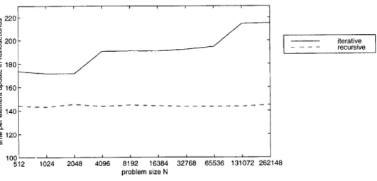
6.4 Experimental results ...

7 Cache complexity of ordinary algorithms 7.1 Matrix multiplication ...

7.2 Matrix transposition ...

7.3 Mergesort ...

8 Other cache models

8.1 Two-level models ...

8.2 Multilevel ideal caches . . . . 8.3 The SUMH model . . . .

8.4 The HMM model . . . .

9 Related work

10 Conclusion

10.1 Engineering cache-oblivious algorithms

10.2 Cache-oblivious data structures ...

10.3 Complexity of cache obliviousness . ... 10.4 Compiler support for divide-and-conquer

10.5 The future of divide-and-conquer ... A Bibliograpy 9 13 19 23 29 35 . . . . 36 . . . . 37 . . . . 41 . . . . 43 45 . . . . 47 . . . . 48 . . . . 49 51 .. ... . 51 . . . . 52 . . . . 53 . . . . 54 57 59 . . . . 60 . . . . 61 . . . . 62 . . . . 63 . . . . 64 67

SECTION 1

Introduction

Resource-oblivious algorithms that nevertheless use resources efficiently offer ad-vantages of simplicity and portability over resource-aware algorithms whose source usage must be programmed explicitly. In this thesis, we study cache re-sources, specifically, the hierarchy of memories in modern computers. We exhibit several "cache-oblivious" algorithms that use cache as effectively as "cache-aware" algorithms.

Before discussing the notion of cache obliviousness, we introduce the (Z, L)

ideal-cache model to study the cache complexity of algorithms. This model, which

is illustrated in Figure 1-1, consists of a computer with a two-level memory hier-archy consisting of an ideal (data) cache of Z words and an arbitrarily large main memory. Because the actual size of words in a computer is typically a small, fixed size (4 bytes, 8 bytes, etc.), we shall assume that word size is constant; the par-ticular constant does not affect our asymptotic analyses. The cache is partitioned into cache lines, each consisting of L consecutive words that are always moved together between cache and main memory. Cache designers typically use L > 1, banking on spatial locality to amortize the overhead of moving the cache line. We shall generally assume in this thesis that the cache is tall:

Z = Q(L2), (1.1)

which is usually true in practice.

The processor can only reference words that reside in the cache. If the refer-enced word belongs to a line already in cache, a cache hit occurs, and the word is

Main organized by Memory optimal replacement

strategy Cache

work W Z/L cache misses Q

Cache

linesI-Lines of length L

Figure 1-1: The ideal-cache model

delivered to the processor. Otherwise, a cache miss occurs, and the line is fetched into the cache. The ideal cache is fully associative [24, Ch. 5]: Cache lines can be stored anywhere in the cache. If the cache is full, a cache line must be evicted. The ideal cache uses the optimal off-line strategy of replacing the cache line whose next access is farthest in the future [7], and thus it exploits temporal locality perfectly.

An algorithm with an input of size n is measured in the ideal-cache model in terms of its work complexity W(n)-its conventional running time in a RAM model [4]-and its. cache complexity Q(n; Z, L)-the number of cache misses it incurs as a function of the size Z and line length L of the ideal cache. When Z and

L are clear from context, we denote the cache complexity as simply Q(n) to ease

notation.

We define an algorithm to be cache aware if it contains parameters (set at ei-ther compile-time or runtime) that can be tuned to optimize the cache complexity for the particular cache size and line length. Otherwise, the algorithm is cache

oblivious. Historically, good performance has been obtained using cache-aware

algorithms, but we shall exhibit several cache-oblivious algorithms for fundamen-tal problems that are asymptotically as efficient as their cache-aware counterparts. To illustrate the notion of cache awareness, consider the problem of multiply-ing two n x n matrices A and B to produce their n x n product C. We assume that the three matrices are stored in row-major order, as shown in Figure 2-1(a). We further assume that n is "big," i.e., n > L, in order to simplify the analysis. The conventional way to multiply matrices on a computer with caches is to use

a blocked algorithm [22, p. 45]. The idea is to view each matrix M as

ing of (n/s) x (n/s) submatrices Mij (the blocks), each of which has size s x s, where s is a tuning parameter. The following algorithm implements this strategy:

BLOCK-MULT (A, B, C, n) 1 for i +- 1 to n/s

2 do for

j

<- 1 to n/s

3 do fork <- 1 to n/s

4 do ORD-MULT (Aik, Bkj;, Cijs)

where ORD-MULT (A, B, C, s) is a subroutine that computes C <- C + AB on s x s matrices using the ordinary O(s3) algorithm (see Section 7.1). (This algorithm as-sumes for simplicity that s evenly divides n. In practice, s and n need have no special relationship, which yields more complicated code in the same spirit.)

Depending on the cache size of the machine on which BLOCK-MULT is run, the parameter s can be tuned to make the algorithm run fast, and thus BLOCK-MULT is a cache-aware algorithm. To minimize the cache complexity, we choose s as large as possible such that the three s x s submatrices simultaneously fit in

cache. An s x s submatrix is stored on 8(s

+

s2

_/L)

_{cache lines. From the} tall-cache assumption (1.1), we can see that s = 8(V'Z). Thus, each of the calls to ORD-MULT runs with at most Z/L =

e(s

+ s2/L) cache misses needed to bring the three matrices into the cache. Consequently, the cache complexity of the entire algorithm is

e(n

+ n2/L + (n/x/Z)3(Z/L)) = 8(n + n2/L + n3/Lv/Z), since the

algorithm must read n2 _{elements, which reside on}

_[n

2_{/L] cache lines.}

The same bound can be achieved using a simple cache-oblivious algorithm that requires no tuning parameters such as the s in BLOCK-MULT. We present such an algorithm, which works on general rectangular matrices, in Section 2. The prob-lems of computing a matrix transpose and of performing an FFT also succumb to remarkably simple algorithms, which are described in Section 3. Cache-oblivious sorting poses a more formidable challenge. In Sections 4 and 5, we present two sorting algorithms, one based on mergesort and the other on distribution sort, both of which are optimal. Section 6 compares an optimal recursive algorithm with an "ordinary" iterative algorithm, both of which compute a multipass filter over one-dimensional data. It also provides some brief empirical results for this problem. In Section 7, we show that the ordinary algorithms for matrix transposition, matrix multiplication, and sorting are not cache optimal.

The ideal-cache model makes the perhaps-questionable assumption that mem-ory is managed automatically by an optimal cache replacement strategy. Although the current trend in architecture does favor automatic caching over programmer-specified data movement, Section 8 addresses this concern theoretically. We show

that the assumptions of two hierarchical memory models in the literature, in which memory movement is programmed explicitly, are actually no weaker than ours. Specifically, we prove (with only minor assumptions) that optimal cache-oblivious algorithms in the ideal-cache model are also optimal in the hierarchical memory model (HMM) [1] and in the serial uniform memory hierarchy (SUMH) model [5, 42]. Section 9 discusses related work, and Section 10 offers some concluding remarks.

Many of the results in this thesis are based on a joint paper [21] coauthored by Matteo Frigo, Charles E. Leiserson, and Sridhar Ramachandran.

SECTION 2

Matrix multiplication

This section describes and analyzes an algorithm for multiplying an m x n matrix by an n x p matrix cache-obliviously using 8(mnp) work and incurring 8(m + n + p

+

(mn + np

+

mp)/L + mnp/LV/Z) cache misses. These results require the

tall-cache assumption (1.1) for matrices stored in row-major layout format, but the assumption can be relaxed for certain other layouts. We also show that Strassen's algorithm [38] for multiplying n x n matrices, which uses (8(nl27) work, incurs

E(1 + n2_{/L + nlo2}7_{/Lv/Z) cache misses.}

The following algorithm extends the optimal divide-and-conquer algorithm for square matrices described in [9] to rectangular matrices. To multiply an m x n ma-trix A by an n x p mama-trix B, the algorithm halves the largest of the three dimensions and recurs according to one of the following three cases:

AB = A1 B= A1B, (2.1)

(A2) A2B)

AB =

(A

₁ A₂) - A₁B₁ + A2B2 , (2.2)

AB = A (B1 B2) = (AB1 AB2) . (2.3)

In case (2.1), we have m > max

{n,

p}. Matrix A is split horizontally, and both halves are multiplied by matrix B. In case (2.2), we have n > max{m, p}. Both

matrices are split, and the two halves are multiplied. In case (2.3), we have p max {im, n}. Matrix B is split vertically, and each half is multiplied by A. For square matrices, these three cases together are equivalent to the recursive multiplication

(a) 1-2-3-4-5-6 8 (b) 1 7 A 57 (c) 0%&2~ 3~ & 2 _(d 2_ 3"642 3 8 348- 0-21-5 6 3 4702 6 24720 4/ 2 2 4 4x44 48 4

Figure 2-1: Layout of a 16 x 16 matrix in (a) row major, (b) column major, (c) 4 x 4-blocked, and (d) bit-interleaved layouts.

algorithm described in [9]. The base case occurs when m = n = p =1, in which case the two elements are multiplied and added into the result matrix.

Although this straightforward divide-and-conquer algorithm contains no tun-ing parameters, it uses cache optimally. To analyze the algorithm, we assume that the three matrices are stored in row-major order, as shown in Figure 2-1(a). In-tuitively, the cache-oblivious divide-and-conquer algorithm uses the cache effec-tively, because once a subproblem fits into the cache, its smaller subproblems can be solved in cache with no further cache misses.

T heorem 1 The cache-oblivious matrix multiplication algorithm uses J( mn p) work and

incurs G(m

+

n

+

p

+

(inn

+

n p

+

m p)/L

+

mn p/ Ly'Z ) cache misses when multiplying an m x n by an n x p matrix.

Proof. It can be shown by induction that the work of this algorithm is 8(mnp).

To analyze the cache misses, let a~ be a constant sufficiently small that three sub-matrices of size m' x n', n' x p', and m' x p', where max{m', n', p'} <; axZ, all fit completely in the cache. We distinguish the following four cases cases depending on the initial size of the matrices.

Case I: m, n, p > cxx/rZ.

This case is the most intuitive. The matrices do not fit in cache, since all dimensions are "big enough." The cache complexity of matrix multiplication can be described by the recurrence

{

((mn+np+mp)/L) if (mn+np+mp) < aZ,

2Q(m/2, n, p) + 0(1) otherwise and if m> n and m >p, 2Q(m, n/2, p) + 0(1) otherwise and if n > m and n >p, 2Q(m,n,p/2) + 0(1) otherwise.

(2.4) The base case arises as soon as all three submatrices fit in cache. The total number of lines used by the three submatrices is e((mn + np

+

mp)/L). The only cache misses that occur during the remainder of the recursion are the

E((mn

+

np

+

mp)/L) cache misses required to bring the matrices into cache.

In the recursive cases, when the matrices do not fit in cache, we pay for the cache misses of the recursive calls, which depend on the dimensions of the matrices, plus 0(1) cache misses for the overhead of manipulating submatri-ces. The solution to this recurrence is Q(m, n, p) = 8(mnp/Lv/Z).

Case II: (m < a/Z and n, p > acZ) OR (m < ajZ and n, p > cx/Z) OR (p < a/Z and m, n > a/Z).

Here, we shall present the case where m < a/rZ and n, p > av/'Z. The proofs for the other cases are only small variations of this proof. The multiplication algorithm always divides n or p by 2 according to cases (2.2) and (2.3). At some point in the recursion, both are small enough that the whole problem fits into cache. The number of cache misses can be described by the recur-rence

E(1+n+np/L + m) if n, p e [a/Z/2,axZ] ,

Q(m, n, p) 2Q(m,n/2,p) +0(1) otherwise andif n > p,

2Q(m, n, p/2) +0(1) otherwise. The solution to this recurrence is 8(np/L + mnp/L /Z).

Case III: (n, p < aZ and m > av/Z) OR (m, p < a1 and n > a/Z) OR

(m, n < xZ and p > av/Z).

In each of these cases, one of the matrices fits into cache, and the others do not. Here, we shall present the case where n, p < axvZ and m > a/'Z. The other cases can be proven similarly. The multiplication algorithm always

divides m by 2 according to case (2.1). At some point in the recursion, m is in the range ox'Z/2 < m <

av/Z, and the whole problem fits in cache. The

number cache misses can be described by the recurrence

Q{n)

< 8(1+m) if m E [aVZ/2,aViZ1 , -m) 2Q(m/2,n,p)+O(1) otherwise;

whose solution is Q(m, n, p) =

O(m

+

mnp/Lx/Z). Case IV: m, n, p < cav'Z.

From the choice of cx, all three matrices fit into cache. The matrices are stored on E)(1 + mn/L + np/L + mp/L) cache lines. Therefore, we have Q(m, n, p) =

8(1 + (mn + np + mp)/L). E

We require the tall-cache assumption (1.1) in these analyses, because the matri-ces are stored in row-major order. Tall caches are also needed if matrimatri-ces are stored in column-major order (Figure 2-1(b)), but the assumption that Z = f(L 2_{) can be}

relaxed for certain other matrix layouts. The s x s-blocked layout (Figure 2-1(c)), for some tuning parameter s, can be used to achieve the same bounds with the weaker assumption that the cache holds at least some sufficiently large constant number of lines. The cache-oblivious bit-interleaved layout (Figure 2-1(d)) has the same advantage as the blocked layout, but no tuning parameter need be set, since submatrices of size 8( vr x vET) are cache-obliviously stored on one cache line. The advantages of bit-interleaved and related layouts have been studied in [18] and [12, 13]. One of the practical disadvantages of bit-interleaved layouts is that index calculations on conventional microprocessors can be costly.

For square matrices, the cache complexity Q(n) = E(n + n2

_/L

_{+ n}3_{/LV/Z) of the}

cache-oblivious matrix multiplication algorithm is the same as the cache complex-ity of the cache-aware BLOCK-MULT algorithm and also matches the lower bound by Hong and Kung [25]. This lower bound holds for all algorithms that execute

the 8(n3) operations given by the definition of matrix multiplication

n

ci; = aikbk;

k=1

No tight lower bounds for the general problem of matrix multiplication are known. By using an asymptotically faster algorithm, such as Strassen's algorithm [38] or one of its variants [45], both the work and cache complexity can be reduced. When multiplying n x n matrices, Strassen's algorithm, which is cache oblivious,

requires only 7 recursive multiplications of n/2 x n/2 matrices and a constant number of matrix additions, yielding the recurrence

(81+n

2/L in2 < CZ

Q(n)

< if n -(1±n+n/L) Z (2.5) -l7Q(n/2) + O(n2_{/L) otherwise}

where a is a sufficiently small constant. The solution to this recurrence is

G(n

+

n2/L + nlos27 _/

L /Z)

Summary

In this section we have used the ideal-cache model to analyze two algorithms for matrix multiplication. We have described an efficient cache-oblivious algo-rithm for rectangular matrix multiplication and analyzed the cache complexity of Strassen's algorithm.

SECTION

3

Matrix transposition and FFT

This section describes an optimal cache-oblivious algorithm for transposing an

m x n matrix. The algorithm uses 8(mn) work and incurs 8(1

+

mn/L) cache

misses. Using matrix transposition as a subroutine, we convert a variant [44] of the "six-step" fast Fourier transform (FFT) algorithm [6] into an optimal cache-oblivious algorithm. This FFT algorithm uses O(n lg n) work and incurs 0(1

+

(n/L)

(1 + logzn)) cache misses.

The problem of matrix transposition is defined as follows. Given an m x n ma-trix stored in a row-major layout, compute and store AT into an n x m mama-trix B also stored in a row-major layout. The straightforward algorithm for transposition that employs doubly nested loops incurs 8(mn) cache misses on one of the matrices when mn

>

Z, which is suboptimal.

Optimal work and cache complexities can be obtained with a divide-and-con-quer strategy, however. If n > m, we partition

A = (A1 A2) , B= .B

(B2)

Then, we recursively execute TRANSPOSE (A1, B1) and TRANSPOSE (A2, B2).

Alter-natively, if m > n, we divide matrix A horizontally and matrix B vertically and likewise perform two transpositions recursively. The next two theorems provide upper and lower bounds on the performance of this algorithm.

Theorem 2 The cache-oblivious matrix-transpose algorithm involves e(mn) work and

Proof. That the algorithm uses 8(mn) work can be shown by induction. For the

cache analysis, let Q(m, n) be the cache complexity of transposing an m x n matrix. We assume that the matrices are stored in row-major order, the column-major case having a similar analysis.

Let x be a constant sufficiently small that two submatrices of size m' x n' and

n' x m', where max{m', n'} < xL, fit completely in the cache. We distinguish the

following three cases. Case I: max{m, n} cL.

Both the matrices fit in 0(1) + 2mn/L lines. From the choice of a, the number of lines required is at most Z/L, which implies Q(m, n) = 0(1 + mn/L). Case II: m i< aL < n OR n < cL < m.

For this case, we assume without loss of generality that m < ctL < n. The case n < aL

<

m is analogous. The transposition algorithm divides the greater dimension n by 2 and performs divide-and-conquer. At some point in the recursion, n is in the range aL/2 K n K aL, and the whole problem fits in cache. Because the layout is row-major, at this point the input array has

n rows, m columns, and it is laid out in contiguous locations, thus requiring

at most 0(1 + nm/L) cache misses to be read. The output array consists of nm elements in m rows, where in the worst case every row lies on a different cache line. Consequently, we incur at most 0(m + nm/L) for writing the output array. Since n > aL/2, the total cache complexity for this base case is

0(1

+ m).

These observations yield the recurrence

Q(m,n)

<( E)(1+m) Q n

{2Q(m,

n/2)

+

0(1) whose solution is Q(m, n) = 8(1 + mn/L). if n E [aL/2,aL] , otherwise ; Case III: m, n > xL.

As in Case II, at some point in the recursion, both n and m fall in the interval

[cL/2, ctL]. The whole problem then fits into cache, and it can be solved with

at most 0(m + n + mn/L) cache misses.

The cache complexity thus satisfies the recurrence

f

0(m + n+n/L) if in,n

E cL2

~ Q(m, n) < 2Q(m/2,n)+-0(1) if i>n ,

2Q(m, n/2) + 0(1) otherwise;

Theorem 3 The cache-oblivious matrix-transpose algorithm is asymptotically optimal. Proof. For an m x n matrix, the matrix-transposition algorithm must write to mn

distinct elements, which occupy at least

[mn/Li

= fl(1

+

mn/L) cache lines. E As an example application of the cache-oblivious transposition algorithm, the rest of this section describes and analyzes a cache-oblivious algorithm for comput-ing the discrete Fourier transform of a complex array of n elements, where n is an exact power of 2. The basic algorithm is the well-known "six-step" variant [6,44] of the Cooley-Tukey FFT algorithm [15]. By using the cache-oblivious transposition algorithm, however, we can make the FFT cache oblivious, and its performance matches the lower bound by Hong and Kung [25].

Recall that the discrete Fourier transform (DFT) of an array X of n complex numbers is the array Y given by

n-1

Y[il =

j

X[j]wn , (3.1)

j=0

where wn = e27r-i/n is a primitive nth root of unity, and 0 < i < n.

Many known algorithms evaluate Equation (3.1) in time O(n lg n) for all inte-gers n [17]. In this thesis, however, we assume that n is an exact power of 2, and compute Equation (3.1) according to the Cooley-Tukey algorithm, which works re-cursively as follows. In the base case where n = 0(1), we compute Equation (3.1)

directly. Otherwise, for any factorization n = n₁n₂ of n, we have n₂-1 ni11

Ylii

+

i2n1] = X[jin2+ j2] 1 on 2

i2=0 ii =0

Observe that both the inner and outer summations in Equation (3.2) are DFT's. Operationally, the computation specified by Equation (3.2) can be performed by computing n2 transforms of size ni (the inner sum), multiplying the result by the

factors wn"j2 (called the twiddlefactors [17]), and finally computing ni transforms

of size n2 (the outer sum).

We choose ni to be 2[sn)/21 and n2 to be 2 (gn)/2J. The recursive step then

operates as follows:

1. Pretend that the input is a row-major ni x n2 matrix A. Transpose A in place,

i.e., use the cache-oblivious algorithm to transpose A onto an auxiliary array

B, and copy B back onto A. (If ni = 2n2, consider the matrix to be made up of records containing two elements.)

2. At this stage, the inner sum corresponds to a DFT of the n2 rows of the

trans-posed matrix. Compute these n2 DFT's of size ni recursively. Observe that,

because of the previous transposition, we are transforming a contiguous ar-ray of elements.

3. Multiply A by the twiddle factors, which can be computed on the fly with no extra cache misses.

4. Transpose A in-place, so that the inputs to the next stage are arranged in contiguous locations.

5. Compute ni DFT's of the rows of the matrix, recursively.

6. Transpose A in-place so as to produce the correct output order.

It can be proven by induction that the work complexity of this FFT algorithm is 0 (n lg n). We now analyze its cache complexity. The algorithm always operates on contiguous data, by construction. In order to simplify the analysis of the cache complexity, we assume a tall cache, in which case each transposition operation and the multiplication by the twiddle factors require at most 0(1 + n/L) cache misses.

Thus, the cache complexity satisfies the recurrence

Q :5

{(n)

O(1+n/L), if n < ctZ (33) n1Q(n2) + n2Q(ni) + 0(1 + n/L) otherwise;

for a sufficiently small constant a chosen such that a subproblem of size aZ fits in cache. This recurrence has solution

Q(n) = 0(1 + (n/L) (1 + logn))

which is asymptotically optimal for a Cooley-Tukey algorithm, matching the lower bound by Hong and Kung [25] when n is an exact power of 2. As with matrix mul-tiplication, no tight lower bounds for cache complexity are known for the general problem of computing the DFT.

Summary

In this section, we have described an optimal cache-oblivious algorithm for FFT. The basic algorithm is the well-known "six-step" variant [6, 44] of the Cooley-Tukey FFT algorithm [15]. By using an optimal cache-oblivious transposition al-gorithm, however, we can make the FFT cache oblivious, and its performance matches the lower bound by Hong and Kung [25].

SECTION 4

Funnelsort

Although it is cache oblivious, algorithms like familiar two-way merge sort (see Section 7.3) are not asymptotically optimal with respect to cache misses. The Z-way mergesort mentioned by Aggarwal and Vitter [3] is optimal in terms of cache complexity, but it is cache aware. This section describes a cache-oblivious sorting algorithm called "funnelsort." This algorithm has an asymptotically optimal work complexity 8 (n lg n), as well as an optimal cache complexity 0(1 + (n

/

L) (1 +

logzn)) if the cache is tall. In Section 5, we shall present another cache-oblivious sorting algorithm based on distribution sort.

Funnelsort is similar to mergesort. In order to sort a (contiguous) array of n elements, funnelsort performs the following two steps:

1. Split the input into n1_/3 _{contiguous arrays of size n}2/3_{, and sort these arrays} recursively.

2. Merge the n1/3 _{sorted sequences using a n'/} 3_{-merger, which is described} be-low.

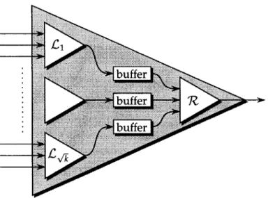
Funnelsort differs from mergesort in the way the merge operation works. Merg-ing is performed by a device called a k-merger, which inputs k sorted sequences and merges them. A k-merger operates by recursively merging sorted sequences that become progressively longer as the algorithm proceeds. Unlike mergesort, however, a k-merger stops working on a merging subproblem when the merged output sequence becomes "long enough," and it resumes working on another merging subproblem.

buffer bufferR buffer

Figure 4-1: Illustration of a k-merger. A k-merger is built recursively out of 'k_ left

A-mergers LI, L2,..., Ek, a series of buffers, and one right /k--merger R.

Since this complicated flow of control makes a k-merger a bit tricky to describe, we explain the operation of the k-merger pictorially. Figure 4-1 shows a repre-sentation of a k-merger, which has k sorted sequences as inputs. Throughout its execution, the k-merger maintains the following invariant.

Invariant The invocation of a k-merger outputs the first k3 elements of the sorted sequence obtained by merging the k input sequences.

A k-merger is built recursively out of VK--mergers in the following way. The k inputs are partitioned into v"k sets of

A

elements, and these sets form the input to the

A

left A-mergers L1, L 2,..., LXk in the left part of the figure. The

out-puts of these mergers are connected to the inout-puts of VK buffers. Each buffer is a FIFO queue that can hold 2k3_/2 _{elements. Finally, the outputs of the buffers are}

connected to the

A

inputs of the right A-merger R in the right part of the figure. The output of this final A-merger becomes the output of the whole k-merger. The reader should notice that the intermediate buffers are overdimensioned. In fact, each buffer can hold 2k3/2 elements, which is twice the number k3/2 _{of elements} output by a A-merger. This additional buffer space is necessary for the correct behavior of the algorithm, as will be explained below. The base case of the recur-sion is a k-merger with k = 2, which produces k3 _{= 8 elements whenever invoked.} A k-merger operates recursively in the following way. In order to output k3

elements, the k-merger invokes R k3/2 times. Before each invocation, however, the k-merger fills all buffers that are less than half full, i.e., all buffers that contain less than k3_/2_{elements. In order to fill buffer i, the algorithm invokes the corresponding}

left merger Li once. Since Li outputs k3

/2 elements, the buffer contains at least k3/2

elements after Li finishes.

In order to prove this result, we need three auxiliary lemmata. The first lemma bounds the space required by a k-merger.

Lemma 4 A k-merger can be laid out in O(k2_{) contiguous memory locations.}

Proof. A k-merger requires O(k2_{) memory locations for the buffers, plus the space} required by the 1k-mergers. The space S(k) thus satisfies the recurrence

S(k) < (V'-k+1)S(V')+0(k 2₎

whose solution is S(k) = 0(k2

). E

It follows from Lemma 4, that a problem of size av/Z can be solved in cache with no further cache misses, where a is a sufficiently small constant.

In order to achieve the bound on the number Q(n) of cache misses, it is im-portant that the buffers in a k-merger be maintained as circular queues of size k. This requirement guarantees that we can manage the queue cache-efficiently, in the sense stated by the next lemma.

Lemma 5 Performing r insert and remove operations on a circular queue causes O(1 + r/L) cache misses iffour cache lines are available for the buffer.

Proof. Associate the two cache lines with the head and tail of the circular queue.

The head- and tail-pointers are kept on two seperate lines. Since the replacement strategy is optimal, it will keep the frequently accessed pointers in cache. If a new cache line is read during an insert (delete) operation, the next L - 1 insert (delete) operations do not cause a cache miss. The result follows. El

Define QM to be the number of cache misses incurred by a k-merger. The next lemma bounds the number of cache misses incurred by a k-merger.

Lemma 6 On a tall cache, one invocation of a k-merger incurs Qm(k) = _{0 (k + k/L + k}3_logzk/L)

cache misses.

Proof. There are two cases: either k < cW'Z or k > av'Z.

Assume first that k < av/Z. By Lemma 4, the data structure associated with the k-merger requires at most O(k2_{) = O(Z) contiguous memory locations. By the} choice of cc the k-merger fits into cache. The k-merger has k input queues, from

which it loads 0(k3) elements. Let ri be the number of elements extracted from the ith input queue. Since k

<

arvZ and L = 0(v/Z), there are at least Z/L = Q(k) cache lines available for the input buffers. Lemma 5 applies, whence the total number of cache misses for accessing the input queues is

k

0

0(1 + ri/L) = O(k + k3/L) .

i=1

Similarly by Lemma 5, the cache complexity of writing the output queue is at most 0(1 + k3

/

L). Finally, for touching the 0(k2_{) contiguous memory locations used by} the internal data structures, the algorithm incurs at most 0(1 + k2

_/L)

_{cache misses.}

The total cache complexity is therefore

Qm(k) = O(k+k 3/L) +0(1+k2 _L)+0(1+k 3_/L)

=

0(k+k

3 _/L)

completing the proof of the first case.

Assume now that k > avZ. In this second case, we prove by induction on k that whenever k > aJZ, we have

QM(k) < (ck3_{logzk)/ L -A(k) , (4.1)}

for some constant c > 0, where A(k) = k(1 + (2clogzk)/L) - o(k3). The

lower-order term A (k) does not affect the asymptotic behavior, but it makes the induction go through. This particular value of A (k) will be justified later in the analysis.

The base case of the induction consists of values of k such that

faZ

1_/4 _{< k <}

avx Z. (It is not sufficient to just consider k =

E(/Z),

since k can become as small as 8(Z1

/

4) in the recursive calls.) The analysis of the first case applies, yielding QM(k) = 0(k+k 3/L). Because k 2 > a/\VZ = f(L) and k = f(1), the last term

dominates, and QM(k) = 0 (k3_{/L) holds. Consequently, a large enough value of c} can be found that satisfies Inequality (4.1).

For the inductive case, let k > av/'Z. The k-merger invokes the v-mergers recursively. Since Va/Z1/4 _<

v/K

_{< k, the inductive hypothesis can be used to}

bound the number QM

(vK)

of cache misses incurred by the submergers. The right merger R is invoked exactly k3/2 _{times. The total number I of invocations of left}

mergers is bounded by 1 < k3/2 + 2v/K. To see why, consider that every invocation of a left merger puts k3/2 elements into some buffer. Since k3 _{elements are output} and the buffer space is 2k2_{, the bound I <} 3 2 ₊

_2VK

_follows.

Before invoking R, the algorithm must check every buffer to see whether it is empty. One such check requires at most

vK

cache misses, since there are

v/K

buffers. This check is repeated exactly k3_/2 _{times, leading to at most k}2 _{cache misses} for all checks.

These considerations lead to the recurrence

QM(k) <

(2k3+ 21k)

QM

(VK) +k 2

Application of the inductive hypothesis yields the desired bound Inequality (4.1), as follows.

QM(k)

<

(2k3/2+21k) Qm(1k) +k 2

2 (k3/2 +

1

k) 2 z - A( )

+

k2

< (ck3_{logzk)/L + k}2 _{(1 + (clogzk)/L)} - (2k3/2 + 21k) A(K-) .

If A(k) k(1 + (2clogzk)/L) (for example), we get

QM(k) < (ck3_{logzk)/L + k}2 _{(1 + (clogzk)/L)} - (2k3/2 + 21K)

1k

_{(1 + (2clogz} k _{) /L)} < (ck3_{logzk)/L + k}2 _{(1 + (clogzk)/L)} - (2k2 _{+ 2k) (1 + (clogzk) /L)} < (ck3_{logzk)/L - (k}2 _{+ 2k) (1 + (clogzk)/ L)} (ck3_{logzk)/L - A(k)}

and Inequality (4.1) follows. l

It can be proven by induction that the work complexity of funnelsort is 0 (n lg n). The next theorem gives the cache complexity of funnelsort.

Theorem 7 Funnelsort sorts n elements incurring at most Q(n) cache misses, where

Q(n)

= 0(1 +(n/L)

(1

+logzn)) .

Proof. If n < aZ for a small enough constant ix, then the funnelsort data structures

fit into cache. To see why, observe that only one k-merger is active at any time. The biggest k-merger is the top-level n1/3-merger, which requires O(n2_/3₎

_<

_0(n) space. The algorithm thus can operate in 0(1 + n/L) cache misses.

If n > cZ, we have the recurrence

Q(n) - n1/3Q(n2/13) + Qm(n1

/3 )

By Lemma 6, we have Qm(n1/3

) - 0(n 1/3 + n/L + (nlogzn)/L).

With the hypothesis Z = f(L 2_{), we have n/L =}

f(ni/ 3). Moreover, we also

have n1

/3 _{= Q(1) and lg n = f(lg Z). Consequently, Qm (n}1

/3

) = 0 ((nlogzn)/L) holds, and the recurrence simplifies to

Q(n) - n1/3Q(n2/3) + 0 ((nlogzn)/L)

The result follows by induction on n. El

This upper bound matches the lower bound stated by the next theorem, prov-ing that funnelsort is cache-optimal.

Theorem 8 The cache complexity of any sorting algorithm is

Q(n)=

fl(1 +(n/L)

(1

+logzn)).

Proof. Aggarwal and Vitter [3] show that there is an ()((n/L)logZ/L(n/Z)) bound

on the number of cache misses made by any sorting algorithm on their "out-of-core" memory model, a bound that extends to the ideal-cache model. By applying the tall-cache assumption Z = fl(L2_{), we have}

Q(n)

> a(n/L)logz/t(n/Z)

> a(n/L) lg(n/Z)/(lg Z - lg L) > a(n/L) lg(n/Z) / lg Z

> a(n/L)lg n/lg Z -- a(n/L) .

It follows that Q(n) = (((n/L)logzn). The theorem can be proven by combining this result with the trivial lower bounds of Q(n) = fl(1) and Q(n) = fl(n/L). l

Corollary 9 The cache-oblivious Funnelsort is asymptotically optimal.

Proof. Follows from Theorems 8 and 7. l

Summary

In this section we have presented an optimal cache-oblivious algorithm based on mergesort. Funnelsort uses a device called a k-merger, which inputs k sorted se-quences and merges them in "chunks". It stops when the merged output becomes "long enough" to resume work on another subproblem. Further, we have shown that any sorting algorithm incurs at least f

(1

+ (n/L) (1 + logzn)) cache misses. This lower bound is matched by both our algorithms.

SECTION

5

Distribution sort

In this section, we describe a cache-oblivious optimal sorting algorithm based on distribution sort. Like the funnelsort algorithm from Section 4, the distribution-sorting algorithm uses O(n lg n) work to sort n elements, and it incurs

8

(1

+(n/L)

(1

+logzn)) .

cache misses if the cache is tall. Unlike previous cache-efficient distribution-sorting algorithms [1, 3, 30, 42, 44], which use sampling or other techniques to find the partitioning elements before the distribution step, our algorithm uses a "bucket-splitting" technique to select pivots incrementally during the distribution.

Given an array A (stored in contiguous locations) of length n, the cache-oblivi-ous distribution sort sorts A as follows:

1. Partition A into \/H contiguous subarrays of size

VH.

Recursively sort each subarray.

2. Distribute the sorted subarrays into q

< /

buckets B1, B2,..., Bq of size n1, n2, ... , nq, respectively, such that for i = 1, 2,... , q - 1, we have

1. max{x

I

x E Bi} < min{x

I

x E Bai}, 2. ni < 2V .

(See below for details.)

3. Recursively sort each bucket.

A stack-based memory allocator is used to exploit spatial locality. A nice prop-erty of stack based allocation is that memory is not fragmented for problems of small size. So if the space complexity of a procedure is S, only 0(1 + S/L) cache misses are made when S < Z, provided the procedure accesses only its local vari-ables.

Distribution step

The goal of Step 2 is to distribute the sorted subarrays of A into q buckets B1,

B2,..., Bq. The algorithm maintains two invariants. First, each bucket holds at

most 26n elements at any time, and any element in bucket Bi is smaller than any element in bucket Bi+i. Second, every bucket has an associated pivot, a value which is greater than all elements in the bucket. Initially, only one empty bucket exists with pivot oo. At the end of Step 2, all elements will be in the buckets and the two conditions (a) and (b) stated in Step 2 will hold.

The idea is to copy all elements from the subarrays into the buckets cache effi-ciently while maintaining the invariants. We keep state information for each sub-array and for each bucket. The state of a subsub-array consists of an index next of the next element to be read from the subarray and a bucket number bnum indicating where this element should be copied. By convention, bnum = oo if all elements in

a subarray have been copied. The state of a bucket consists of the bucket's pivot and the number of elements currently in the bucket.

We would like to copy the element at position next of a subarray to bucket

bnum. If this element is greater than the pivot of bucket bnum, we would

incre-ment bnum until we find a bucket for which the eleincre-ment is smaller than the pivot. Unfortunately, this basic strategy has poor caching behavior, which calls for a more complicated procedure.

The distribution step is accomplished by the recursive procedure DISTRIBUTE.

DISTRIBUTE (i,

j,

m) distributes elements from the ith through (i + m - 1)th sub-arrays into buckets starting from Bj. Given the precondition that each subarray

r = i, i +1..., i + m - 1 has its bnum[r] >

j,

the execution of DISTRIBUTE (i,

j,

m)

enforces the postcondition that bnum [r] >

j

+ m. Step 2 of the distribution sort in-vokes DISTRIBUTE (1,1,

Vi).

The following is a recursive implementation of

DISTRIBUTE (i,

j,

m) 1 ifm=1

2 then CoPYELEMS (i,

j)

3 else DISTRIBUTE (i,

j,

m/2)

4 DISTRIBUTE (i + m/2,

j,

m/2)

5 DISTRIBUTE (i,

j

+ m/2, m/2)

6 DISTRIBUTE (i + m/2,

j

+ m/2, m/2)

In the base case (line 1), the subroutine COPYELEMS(i,

j)

copies all elements from subarray i that belong to bucket

j.

If bucket

j

has more than 2VH elements after the insertion, it can be split into two buckets of size at least ,. For the splitting oper-ation, we use the deterministic median-finding algorithm [16, p. 189] followed by

a partition. The next lemma shows that the median-finding algorithm uses O(m) work and incurs 0(1 + m/L) cache misses to find the median of an array of size m. (In our case, we have m > 2V + 1.) In addition, when a bucket splits, all sub-arrays whose bnum is greater than the bnum of the split bucket must have their bnum's incremented. The analysis of DISTRIBUTE is given by the following two lemmata.

Lemma 10 The median of m elements can be found cache-obliviously using O(m) work and incurring 0(1 + m/L) cache misses.

Proof. See [16, p. 189] for the linear-time median finding algorithm and the work analysis. The cache complexity is given by the same recurrence as the work com-plexity with a different base case.

Q(m)

{

0(1+m/L) if m

<

aZ,

Q([m/5)

+ Q(7m/1O + 6) + 0(1 + m/L) otherwise,

where a is a sufficiently small constant. The result follows. El

Lemma 11 Step 2 uses O(n) work, incurs 0(1 + n/L) cache misses, and uses O(n) stack space to distribute n elements.

Proof. In order to simplify the analysis of the work used by DISTRIBUTE, assume that CoPYELEMS uses 0(1) work. We account for the work due to copying ele-ments and splitting of buckets separately. The work of DISTRIBUTE on m subarrays is described by the recurrence

It follows that T(m) 0 O(m2_{), where m = \/H initially.}

We now analyze the work used for copying and bucket splitting. The number of copied elements is O(n). Each element is copied exactly once and therefore the work due to copying elements is also O(n). The total number of bucket splits is at most

vf.

To see why, observe that there are at most -/h buckets at the end of the distribution step, since each bucket contains at least h elements. Each split operation involves 0( .,/H) work and so the net contribution to the work is O(n). Thus, the total work used by DISTRIBUTE is W(n) = O(T(VH)) + O(n) + O(n) O(n).

For the cache analysis, we distinguish two cases. Let a be a sufficiently small constant such that the stack space used by sorting a problem of size aZ, including the input array, fits completely into cache.

Case I: n < cZ.

The input and the auxiliary space of size 0(n) fit into cache using 0(1 + n/L) cache lines. Consequently, the cache complexity is 0(1 + n/L).

Case II: n > aZ.

Let R(m, d) denote the cache misses incurred by an invocation of the subrou-tine DISTRIBUTE(i,

j,

m) that copies d elements from m subarrays to m

buck-ets. We again account for the splitting of buckets separately. We first prove that R satisfies the following recurrence:

R (m, d) < O(L+d/L) if m< cL, (5.1) - ₁

<<4

RR(m/2, di) otherwise,

where 1<i<4 ddj = d.

First, consider the base case m < cxL. An invocation of DISTRIBUTE(i,

j,

m)

operates with m subarrays and m buckets. Since there are f2(L) cache lines, the cache can hold all the auxiliary storage involved and the currently ac-cessed element in each subarray and bucket. In this case there are O(L + d/L) cache misses. The initial access to each subarray and bucket causes

0(m) = 0(L) cache misses. The cache complexity for copying the d elements from one set of contiguous locations to another set of contiguous locations is 0(1 + d/L), which completes the proof of the base case. The recursive case, when m > aL, follows immediately from the algorithm. The solution for Recurrence 5.1 is R(m, d) = O(L

+

m2/L + d/L).

We still need to account for the cache misses caused by the splitting of buck-ets. Each split causes 0(1+

VH/L)

cache misses due to median finding

(Lemma 10) and partitioning of V/h contiguous elements. An additional 0(1 + VI//L) misses are incurred by restoring the cache. As proven in the

work analysis, there are at most f/h split operations.

By adding R(

vl,

n) to the complexity of splitting, we conclude that the total

cache complexity of the distribution step is O(L + n/L + V/In(1 + x//L))

0(n/L).

El Theorem 12 Distribution sort uses O(n lg n) work and incurs 0(1 + (n/L) (1+ logzn)) cache misses to sort n elements.

Proof. The work done by the algorithm is given by

W(n) = VnW(VH) + W(ni) + O(n),

where q <

v'H,

each ni < 2k/n, and ~ q> ni n. The solution to this recurrence is

W(n) = 0(n lg n).

The space complexity of the algorithm is given by

S(n) S(2Vn) + 0(n) .

Each bucket has at most 2/n elements, thus the recursive call uses at S (2fn) space and the O(n) term comes from Step 2. The solution to this recurrence is S(n) =

O(n).

The cache complexity of distribution sort is described by the recurrence

0(1+n/L) if n < aZ,

q

Q(n)

<

VQ(V)

+ _{Q(ni) + 0(1 + n/L) otherwise ,}

where a is a sufficiently small constant such that the stack space used by a sorting problem of size aZ, including the input array, fits completely in cache. The base case n < ctZ arises when both the input array A and the contiguous stack space of size S(n) = O(n) fit in 0(1 + n/L) cache lines of the cache. In this case, the algorithm incurs 0(1

+

n/L) cache misses to touch all involved memory locations

once. In the case where n > aZ, the recursive calls in Steps 1 and 3 cause

Q

(

s/H) +

F~_ Q(ni) cache misses and 0(1 + n/L) is the cache complexity of Steps 2 and 4,

as shown by Lemma 11. The theorem now follows by solving the recurrence. El Corollary 13 The cache-oblivious distribution sort algorithm is asymptotically optimal.

Summary

In this section, we have presented another optimal cache-oblivious sorting algo-rithm, which is based on distribution sort. All previous cache-efficient distribution sort algorithms [1, 3,30,42,44] are cache aware, since they are designed for caching models where the data is moved explicitly. They usually use a sampling processes to find the partitioning elements before the distribution step. Our algorithm finds the pivots incrementally during the distribution.

SECTION 6

Jacobi multipass filter

This section compares an optimal recursive algorithm with a more straightforward iterative algorithm, both which compute a multipass filter over one-dimensional data. When computing n generations on n elements, both algorithms use

0(n

2

)

work. The iterative incurs E(n 2_{/L) cache misses, if the data does not fit into the}

cache, where the recursive algorithm incurs only 8(1 + n/L

+

n2 /ZL) cache misses

which we prove to be cache optimal. We also provide some brief empirical results for this problem. The recursive algorithm executes in less than 70% of the time of the iterative algorithm for problem sizes that do not fit in L2-cache

Consider the problem of a computing a multipass filter on an array A of size

n, where a new value A('' at generation T + 1 is computed from values at the

previous step T according to some update rule. A typical update function is

A +- (Ad + Ai + Ai+)) _+ _ /3. (6.1)

Applications of multipass filtering include the Jacobi iteration for solving heat-diffusion equations [31, p. 673] and the simulation of lattice gases with cellular automata. These applications usually deal with multidimensional data, but here, we shall explore the one-dimensional case for simplicity, even though caching ef-fects are often more pronounced with multidimensional data.

JACOBI-ITER(A) 1 n<-lengthof A 2 fori<-1ton/2

3 do for

j

<- 1 to n > Generation 2i

4 do tmp[j] +- (A[(j - 1) mod n] + A[j] + A[(j+ 1) mod n]) /3

5 for j <- 1 to n > Generation 2i +1

6 do A[j] <- (tmp[(j - 1) mod n] + tmp[j] + tmp[(j+ 1) mod n]) /3 Figure 6-1: Iterative implementation of n-pass Jacobi update on array A with n elements.

6.1 Iterative algorithm

We first analyze the cache complexity of the straightforward implementation JA-COBI-ITER of the update rule given in Equation (6.1). We show that this algorithm, shown in Figure 6-1, uses 8(n) temporary storage and performs 6(n2 _{) memory}

accesses for an array of size n. If the array of size n does not fit into cache, the total number of cache misses is 6 (n2

_/

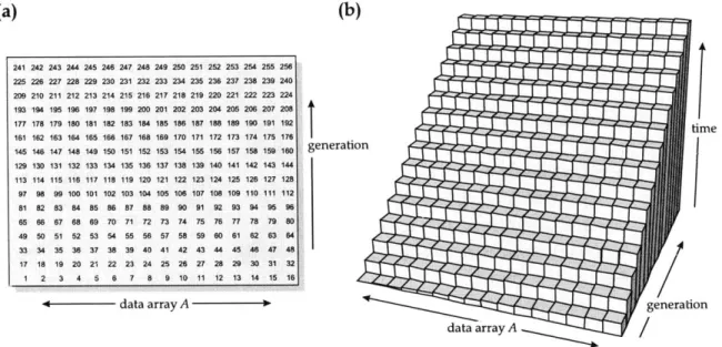
_L).

To illustrate the order of updates of JACOBI-ITER on input A of size ni, we view

the computation of n generations of the multipass as a two-dimensional trace ma-trix

T

of size n x n. One dimension of T is the offset in the input array and the other dimension is the "generation" of the filtered result. The value of element

T4,2 is the value of array element A[2] at the 4th generation of the iterative

algo-rithm. One row in the matrix represents the updates on one element in the array. The trace matrix of the iterative algorithm on a data array of size 16 is shown in Figure 6-2. The height of a bar represents the ordering of the updates, where the higher bars are updated later. The bigger the difference in the height of two bars, the further apart in time are their updates. If the height of a bar is not much bigger than the height of the bar directly in front of it, it is likely that the element is still in cache and a hit occurs. The height differences between two updates to the same el-ement in the iterative algorithm are all equal. Either the updates are close enough together that all updates are cache hits, or they are too far apart, and all updates are cache misses.

Theorem 14 The JACOBI-ITER algorithm uses 6( n2_{) work when computing n}

genera-tions on an array of size n. JACOBI-ITER incurs 6(1 + n/L) cache misses if the data fits into cache, and it incurs 6(n2_{/L) cache misses if the array does not fit into cache.}

Proof. Since there are two nested loops, each of which performs n iterations, the