UNIVERSITÉ DU QUÉBEC À MONTRÉAL
DEPARTMENTOF EARTH AND ATMOSPHERIC SCIENCES
NEAR-SURFACE WIND DATA ASSIMILATION USING A GEO-STATISTICAL OBSERVATION OPERA TOR
THE SIS
PRESENTED AS PARTIAL FULFILMENT OF THE REQUIREMENTS FOR THE DOCTORAL PROGRAM IN
EARTH AND ATMOSPHERIC SCIENCES
BY JOËLBÉDARD
FINAL SUBMISSION MONTRÉAL, NOVEMBER 2015
UNIVERSITÉ DU QUÉBEC À MONTRÉAL Service des bibliothèques
Avertissement
La diffusion de cette thèse se fait dans le respect des droits de son auteur, qui a signé le formulaire Autorisation de reproduire et de diffuser un travail de recherche de cycles supérieurs (SDU-522 - Rév.07 -2011). Cette autorisation stipule que «conformément
à
l'article 11 du Règlement no 8 des études de cycles supérieurs, [l'auteur] concèdeà
l'Université du Québecà
Montréal une licence non exclusive d'utilisation et de publication de la totalité ou d'une partie importante de [son] travail de recherche pour des fins pédagogiques et non commerciales. Plus précisément, [l'auteur] autorise l'Université du Québec à Montréalà
reproduire, diffuser, prêter, distribuer ou vendre des copies de [son] travail de rechercheà
des fins non commerciales sur quelque support que ce soit, y compris l'Internet. Cette licence et cette autorisation n'entraînent pas une renonciation de [la] part [de l'auteur] à [ses] droits moraux ni à [ses] droits de propriété intellectuelle. Sauf entente contraire, [l'auteur] conserve la liberté de diffuser et de commercialiser ou non ce travail dont [il] possède un exemplaire.»- -- - - -- - -- -- · -
-UNIVERSITÉ DU QUÉBEC À MONTRÉAL
DÉPARTEMENT DES SCIENCES DE LA TERRE ET DE L'ATMOSPHÈRE
ASSIMILATION DES VENTS DE SURF ACE À L'AIDE D'UN OPERATEUR D'OBSERVATION GÉO-STA TISTIQUE
THÈSE
PRÉSENTÉ COMME EXIGENCE PARTIELLE AU PROGRAMME DE DOCTORAT EN SCIENCES DE LA TERRE ET DE L'ATMOSPHÈRE
PAR JOËLBÉDARD
DÉPOTFINAL
ACKNOWLEDGEMENTS
1 would like to thank my directors Prof. Pierre Gauthier (UQAM) and Dr. Stéphane Laroche (Environment Canada) for their advice and support in carrying out this work. More specifically, 1 am grateful to have had both give me the opportunity to work with them, as weil as for their teachings and scientific supervision. Very special thanks to Dr. Laroche for his devotion to the project and to Prof. Gauthier for introducing me to different parties involved in data assimilation internationally. 1 also wish to thank Mr. Alain Forcione from IREQ and Dr. Wei Yu from Environment Canada who initiated this research project. Many thanks to Mr. Forcione for his support regarding the. access to the tati anemometer tower observations from wind farms.
Thanks to Dr. Mark Buehner, Dr. Peter Houtekamer, and other colleagues from Environment Canada for their technical support and advices. Also, thanks to Mr. Michel Valin from the ESCER Center for many fruitful discussions. Moreover, thanks to the members of the present jury for their precious comments and their judicious evaluation.
On a persona( note, very special thanks are reserved to Gabrielle, my family and my friends for being with me, for your constant support and your infinite patience.
This project is funded by the Natural Sciences and Engineering Research Council of Canada (NSERC), the Hydra-Québec research institute (IREQ) and the Meteorological Research Division of Environment Canada. The author also acknowledges the contributions of the ESCER Centre (UQAM) in this research program.
TABLE OF CONTENT
LIST OF FIGURES ... VIII LIST OF TABLES ... XII
RÉSUMÉ ... XIII ABSTRACT ... XVI
INTRODUCTION ... 1
1.1. MOTIVATION ... 1
1.2. WIND POWER FORECASTING ... 2
1.3. OBJECTIVES AND METI-IODOLOGY ... 4
CHAPTER II ... 9
EXPERIMENTAL FRAMEWORK ... 9
2.1. DATAASSlMlLATION ... ! ... 9
2.1.1. Background error covariances ... 11
2.1.2. Observation error covariances ... 12
2.2. EXPERJMENTAL SETUP ... 13
2.2.1. Data assimilation system ... 13
2.2.2. Cycling experiments with the operational systems ... 15
2.2.3. Simplified non-cycling experiments ... 16
v
CHAPTER III
A GEO-STA TISTICAL OBSERVATION OPERA TOR
FOR THE ASSIMILATION OF NEAR-SURFACE WIND DATA ... 00 ... 20
ABSTRACT ... 22
3.1. INTRODUCTION ... 00 ... 23
3.2. DATA ASSIMILATION SYSTEM ... oo ... 26
3 .2.1. Background error statistics ... 00.26 3.3. MEASUREMENT ERROR STATISTICS 0000000000000000000000000000oooooooooooooooooooooooooooooooooooooooooooooooo29 3 .4. OBSERVATION OPERA TOR 000000000000000000000000000000000000 00000000 0000 OOOOOOOOOOOOOOoooooooooooo 000000000000000031 3.4.1. Observation operator design 0000000000000000oooooooooooooooooooooooooooooooooooooooooooooooooooooooooooo.31 3.4.2. Training and statistical robustness of statistical operators000000000000000000oooooooooooooo33 3 .4.3. Temporal variabil ity. oo. 00 00000000000000000000000000000000 .. 00000000.000000000000 oo• .. oooooo•. oo•. 0000000000003 5 3.4.4. Representativeness error correction •oooooooooooooooooooooooooooooooooooooooooooooo.oooooooooooooooooo35 3.4.5. Observation error statisticsoo.oooooooooooo .. oo.oooooooooooooooooooooooooooooooooooooooooooooooooooooooooo . .40 3.4.6. Tangent linear and adjoint modelsoooooooooooooooooooooooooooooooooooooooooooooooooooooooooooooooooooo41 3.5. OBSERVATION ERROR CORRELATIONS ooooooooooooooooooooooooooo ... oooooooooooooooooooooo•oo• ... ooooooooooo.43 3.6. EVALUATION OF THE IMPACT OF OBSERVATION OPERATORSoooooooooooooooooooooooooo .. oooooooooo46 3.7. RESULTS FROM NON-CYCLTNG ASSIMILATION EXPERJMENTSOOOOOOOOOOOOOOOOOOOOOOOOooOOOOoooooooo50 3.8. CONCLUSIONS ···oo···oo··· ... 55
ACKNOWLEDGEMENTS ···oo··oo ... oo .. ·oo· ····oo···oo·· ... 00 ... oo .... 5 8 APPENDIX •••••••oo••···••oo••···••oo••••••••oo••••••••••oo•••···••oo••···59
VI
CHAPTERIV
NEAR-SURFACE WIND DATA ASSIMILATION:
TEMPORAL PROPAGATION OF THE ANAL YSIS INCREMENT
AND MUL TIV ARIA TE IMPACT ON FORECASTS 00 oo ... 66 ABSTRACT ... 68 4.1. INTRODUCTION ... 000 ... oo .. 00000000000 0000 .. 00000000000 oo• 000000.000000000000000000 00 0000 00000000000069 4.2. THE DATA ASSIMILATION SYSTEM. 000000 000000000000000000000000.0000 0000000000000000000000 oooooooooooooo.oooo• 72 4.2.1. Geo-statistical observation operator00000000oooooooooooooooooooooooooooooooooo.oooooooooooooooooooooo.73 4.2.2. Observation quality controloooooooooooooo•oo·oo.oooooooooooo•oo•oooooooooooooooooooooooooooooooooooooooooo74 4.2.3. Observation error statisticsooooooooooooooooooo····oo••oooooooooooooooo··oooooooooooooooooooooooooo.oooooooo76 4.2.4. Evaluation dataset ... oo .. oo···oo···oo···oo····oo···oo···oo·78 4.3. SIMPLIFIED ASSIMILATION EXPERIMENTSoooooooooooooooooooooooooooooooo•oo•oo••oooooooooooooooooooooooooo.79 4.3 .1. Evaluation against near-surface wind observations oooooooooooooooooooooooo• 00000 00000000000081 4.3.2. Evaluation against upper-air observations oooooooooooooooooooooooooooooooooooooooooooooooooooooooo87 4.3.3. Impact of the background error covariance components 000000000ooooooooooooooooooooooooo90 4.3.4. Constraining mass field using surface pressure observationsooooooooooooooooooooooooooo91 4.4. EXPERJMENTS WTTH THE OPERATIONAL SYSTEM ooooooooooooooooooooooooooooooooooooooooooooooooooooooo.93
4.4.1. Evaluation against near-surface wind observations 0000000000oooooooooooooooooooooooooooooooo95 4.4.2. Upper-air evaluation ···oo···oo····oo···oo···oo····96 4.5. SUMMARY AND CONCLUSIONS oooooooooooooooooooooooooooooooooooooooo.ooooooooooooooooooooooooooooooooooooooo.1 00 ACKNOWLEDGEMENTS ... 1 04 REFERENCES ···oo··· ... ···oo··· oo ... ·oo·· ... oo ... 1 05
VII
CON.CLUSION ... 1 08
5.1. 0RlGfNALCONTRIBUTIONS ... 108
5.2. SUMMARYOFTHERESULTS ... 110
5 .2.1. Observation operator ... 11 0 5 .2.2. Background error statistics ... 11 0 5.2.3. Multivariate impact ... 111
5.2.4. Observation impact ... 112
5.3. LIMITAT!ONS ... 112
5.4. 0UTLOOK ... 113
LIST OF FIGURES Figure Caption 2.1 3.1 3.2 3.3 3.4 3.5
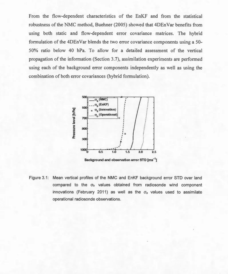
Flow chart diagram of the non-cycling assimilation experiments. Mean vertical profiles of the NMC and EnKF background error STD over land compared to the Gb values obtained from radiosonde wind component innovations (February 2011) as weil as the (Jo values used to assimilate operational radiosonde observations.
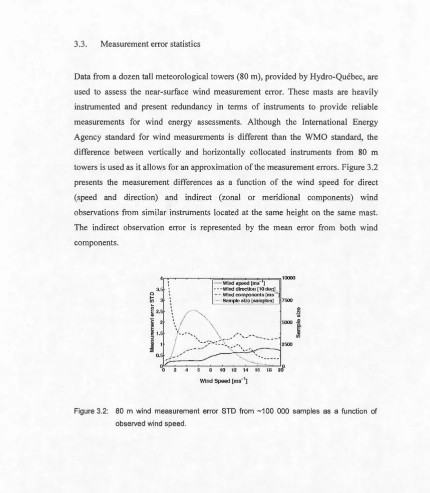
80 m wind measurement error STD from ~ 100 000 sam pies as a function of observed wind speed.
10 m wind components innovation (observed minus background states) bias and STD as a function of the training dataset length using Bilin, Bilin coupled with a MOS, and GMOS. The number of grid-points used for the GMOS operators is specified in parentheses (e.g., 2x2 when using the 4 nearest grid-points).
Frequency distribution of the wind components innovation STD for the 545 SYNOP stations using either Bilin or GMOS operator.
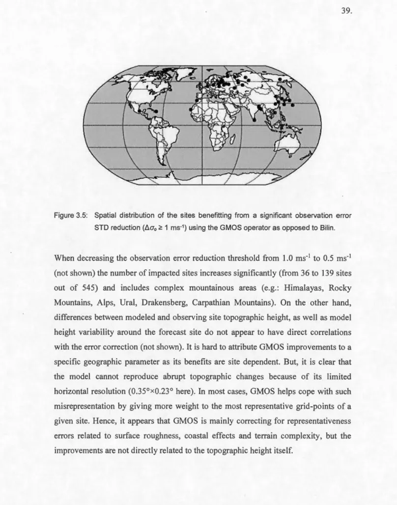
Spatial distribution of the sites benefitting from a significant observation error STD reduction (~(Jo 2: 1 ms-1) using the GMOS operator as opposed to Bi 1 in.
Page 16 28
29
34 38 39IX
3.6 Comparison between tbe wind error metric (lines) and experimental 49 results (symbols) for different observation operators: Bi lin (top left), Bi lin with bias correction (top right), Bilin with both bias and amplitude corrections from MOS (bottom left), and GMOS (bottom right). Results are plotted for different specified values of the representativeness correlation coefficients (rr = 0.0, 0.5, and 1.0). The analysis error variance is shawn as a function of the prescribed observation error variance for each of the experiments. White the symbols represent the experimental results, the li nes are the corresponding representation of the analysis error variance from (3.13) evaluated for three values of the representativeness error correlation.
3.7 Mean observation impact on wind components analysis (evaluated against 52 radiosonde observations) for Bilin and GMOS operators. The dark (light) shaded area presents the 90 % confidence interval for the Bilin (GMOS) operator. From top to bottom, the panels show data assimilation results using static (top), dynamic (centre), or hybrid (bottom) background error statistics.
3.8 Mean zonal wind analysis increments for Bi lin (top) and GMOS operators 54 (bottom).
4.1 Spatial distribution of the 4942 SYNOP sites considered in this study 76 (black dots). The rectangle refers to the area where the upper-air evaluation is performed.
4.2 Frequency distribution of the near-surface wind observation error 77 statistics using the GMOS operator for the 4942 SYNOP stations considered in this study.
4.3 Spatial distribution of the 1487 SYNOP sites (left: black dots) located in 79 the selected domain. This area is densely observed and also includes 124 radiosonde stations used for upper-air evaluation purposes (right: black stars).
4.4 Wind speed departure STD as a function offorecast lead time for different 82 experiments (CNTRL, Bilin and GMOS). Note that the CRTL experiment is post-processed using both Bilin and GMOS in arder to highlight the impact of the operator on post-processing.
x
4.5 Forecast differences (llbVII) between CRTL and the experiments (Bilin: 83 Left panel and GMOS: Right panel) using different background error covariances (Hybrid, NMC and EnKF). Results are presented for the February 151
run launched at 0000 UTC. The upper panels show the results over the whole 48 h forecast period white only the first 6 h are depicted in the lower panels.
4.6 Contribution of the main tenns of Eq. ( 4.3) on evolution of the forecast 86 difference between CNTRL and the experiments (left: GMOSNMc; right: GMOSEnKF). Results for advection, Coriolis effect, horizontal diffusion are omitted as their respective influence is small compared to the pressure gradient, the vertical diffusion and orographie blocking.
4.7 24 h forecast departure bias from hybrid runs as evaluated against 88 radiosonde observations over Europe for wind speed (left) and geopotential height (right).
4.8 Forecast depatture STD from hybrid runs as evaluated against radiosonde 89 observations over Europe for wind speed (left) and geopotential height (right). In each plot, results from 12 h, 24 h, 36 h and 48 h forecasts are shown from left to right respective! y.
4.9 24 h forecast departure bias from GMOS runs as evaluated against 90 radiosonde observation profiles over Europe for wind speed (left) and geopotential height (right).
4.10 24 h forecast departure bias from GMOS runs as evaluated against 92 radiosonde observations over Europe for wind speed (left) and geopotential height (right). The CNTRL experiment is represented by circles, white assimilation experiments using only surface pressure observations (PO), only near-surface wind observations (GMOSEnKF), or both surface pressure and near-surface wind observations (PO
+
GMOSEnKF) are shown by solid, dot and dash tines respectively.4.11 Wind speed departure STD as a function of forecast lead ti me for different 95 experiments (CNTRLosE, BilinosE and GMOSosE). Note that the GMOS operator is also used for post-processing in ali experiments.
Xl
4.12 Mean 12 h forecast departure STD (against own analyses) differences 98 (BilinosE minus GMOSosE) over Europe. Results for 10 m wind speed ([ms-1]) are averaged over the February 2011 period. Positive (negative) values are represented by dark (light) col01·s. A positive value (dark gray) indicates that the GMOSosE experiment is better than BilinosE, while light gray color indicate neutra! results.
4.13 Hovmoller diagram presenting the differences between BilinosE and 100 GMOSosE 12 h forecast departure STD (against own analyses). Results for 10 m wind speed ([ms-1]) are presented through February 2011 for
different longitude bands over Europe. Positive (negative) values are represented by dark (light) col01·s. A positive value (dark gray) indicates that the GMOSosE experiment is better than BilinosE, while light gray color indicate neutra! results.
LIST OF TABLES
Table Caption Page
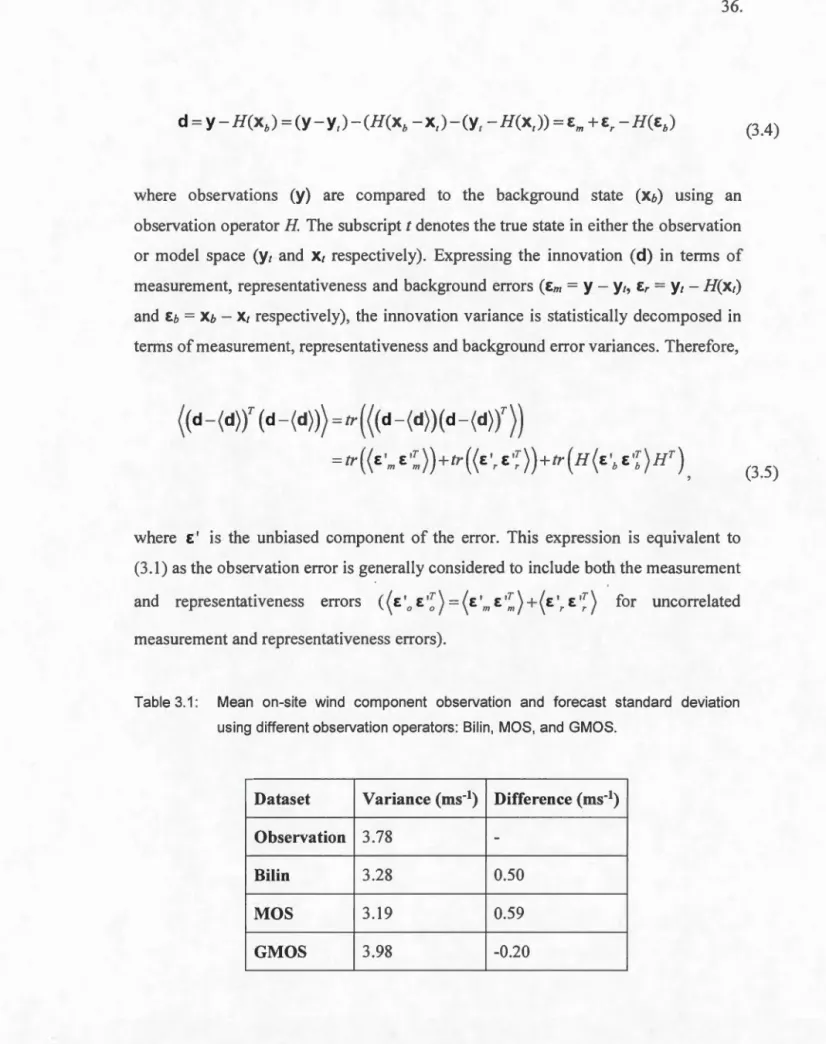
3.1 Mean on-site wind component observation and forecast standard 36 deviation using different observation operators: Bilin, MOS, and GMOS.
3.2 Configuration of the 60 analysis experiments performed. For each 47 observation operators implemented, the different observation error value and background error matrix prescribed to the data assimilation system as weil as the number of experiments are listed.
4.1 Configuration of the 9 simplified data assimilation performed. Each 80 experiment is listed along with its own combination of near-surface wind observation operator, background and observation error statistics prescribed to the data assimilation system as weil as assimilated observations. It is a Iso specified if the experiments are cycled or not.
4.2 Configuration of the 3 cycling OSE performed. Each experiment is 94 listed along with its own combination of near-surface wind observation operator, background and observation error statistics prescribed to the data assimilation system as weil as assimilated observations. lt is also specified if the experiments are cycled or not.
RÉSUMÉ
L'intégration de la production éolienne dans les réseaux électriques comporte
d'importants défis reliés à la variabilité du vent. Afin de garantir la fiabilité du réseau, il faut se doter de réserves de puissance pouvant pallier les effets des variations de cetty ressource. Pour des échéances allant jusqu'à 24 h, une connaissance précise de la production à venir (basée sur la prévision du vent et des paramètres météorologiques connexes) permet de limiter ces réserves au strict minimum, maximisant ainsi la valeur de la ressource éolienne. Les prévisions météorologiques de courte échéance sont imprécises et une partie de l'erreur peut être attribuée aux conditions initiales fournies par les analyses. Malgré la disponibilité d'observations de vent de surface au-dessus des continents, peu d'entre elles sont utilisées dans la production d'analyses en raison des interactions entre la topographie locale et
l'écoulement à fine échelle non-résolu par les modèles météorologiques. La disparité
d'échelles entre les observations et le modèle cause des erreurs de représentativité qui peuvent devenir significatives, particulièrement en terrain complexe.
L'objectif principal de ce projet est d'améliorer les prévisions troposphériques de
courte échéance en assimilant les observations de vents continentaux dans le système
d'assimilation de données ensembliste-variationnel d'Environnement Canada. Un
nouvel opérateur d'observation basé sur les géo-statistiques (GMOS) a été développé dans le but de corriger les erreurs systématiques et de représentativité. Cet opérateur
combine une méthode de correction statistique à une méthodologie utilisant plusieurs
points de grille afin de prendre avantage des corrélations multi-échelles. GMOS est comparée à un opérateur conventionnel basé sur une interpolation bilinéaire (Bilin) dans le contexte d'analyses et de prévisions opérationnelles.
Des expériences d'assimilation ont été effectuées en assimilant les observations de
vents de surface uniquement pour les stations où un radiosondage est également
disponible. Ces expériences avaient pour but de comprendre l'impact de ces
observations sur les analyses météorologiques et ainsi repérer les composantes du
système d'assimilation nécessitant des améliorations afin de profiter du plein
potentiel de ces observations. Les corrections apportées ont été systématiquement
évaluées en comparant les analyses résultantes aux observations des radiosondages.
Ces observations indépendantes n'étaient pas utilisées dans l'assimilation. Cette
méthode de validation a permis d'estimer la variance d'erreur d'observation qui maximise l'impact des observations de vent de surface tout en générant une analyse
XIV.
cohérente avec les observations de radiosondages. Les résultats des expériences d'assimilation (sur une période d'un mois) montrent qu'à cause de la structure verticale des covariances d'erreur de prévision, l'assimilation des vents de surface impacte principalement les basses couches de l'atmosphère. En sélectionnant statistiquement les points de grille du modèle qui sont les plus corrélés aux observations, GMOS permet de mieux représenter les phénomènes météorologiques
in situ, ce qui élimine les biais, réduit les erreurs de représentativité et les corrélations d'erreurs d'observation.
Des résultats sont aussi présentés pour des expériences d'assimilation non cyclées utilisant cette fois les vents de surface de toutes les stations synoptiques globales (SYNOP). La vérification des analyses et des prévisions 48 h à l'aide d'observations de surface démontre que l'utilisation de GMOS permet d'améliorer les prévisions de vent locales. L'impact diminue rapidement et n'est valide que pour des échéances allant jusqu'à 6 h en raison de l'utilisation des statistiques d'erreur de prévision homogènes. Ces statistiques d'erreur génèrent des incréments d'analyse altérant principalement les vents et les paramétrages reliés au blocage orographique et à la couche limite atmosphérique atténuent l'incrément d'analyse. Toutefois, les statistiques d'erreurs dynamiques provenant de méthodes ensemblistes permettent une meilleure propagation de l'information à la verticale puisqu'elles varient en fonction de la stabilité atmosphérique. Elles conduisent aussi à des incréments mieux balancés à cause des corrélations plus accentuées entre les champs de vent et de masse. L'incrément peut alors se propager dans le temps: le gradient de pression généré supporte 1 ~incrément de vent et contrebalance les forces diffusives des paramétrages du modèle. Les statistiques d'erreur de prévisions sont déterminantes pour la propagation de l'information dans les systèmes d'assimilation et de prévision.
En assimilant conjointement les observations de vent et de pression de surface, GMOS permet de réduire le biais des prévisions de vent jusqu'à 48 h. Les résultats de ces expériences suggèrent que la complémentarité entre les observations de vent et de masse, des statistiques d'erreur de prévisions dynamiques et l'opérateur GMOS sont des composantes essentielles à l'utilisation des vents de surface pour l'amélioration des conditions initiales des modèles de prévision numérique.
Enfin, les résultats d'expériences cyclées avec le système d'Environnement Canada utilisant toutes les observations assimilées opérationnellement, auxquelles on ajoute les observations de vents de surface, indiquent que les incréments générés par Bilin
sont atténués par le système alors que ceux générés par GMOS persistent plus
longtemps puisqu'ils sont mieux balancés. Ainsi, les prévisions issues des
expériences employant GMOS (Bi! in) sont plus (moins) cohérentes avec les analyses que les prévisions issues de l'expérience de contrôle n'assimilant pas les vents de surface au-dessus des continents.
xv.
Mots-clés: stattsttques d'erreur d'observation et de prévision, paramétrages de la couche limite atmosphérique, énergie éolienne, assimilation de données de surface, - analyse météorologique, prévision numérique du temps, validation contre analyses et
ABSTRACT
The ability to predict hourly near-surface winds up to 24 h in the future plays a key
rote in the integration of wind power in the energy production of electrical facilities. Improvement in the accuracy of wind power predictions is essential in the overall energy management of a network comprising different energy sources and increases the value of wind energy. From numerical weather prediction assessments, large
forecast errors appear to grow from an inadequate characterisation of the atmosphere in the initial conditions, defined by large-scale analyses, used by a numerical weather
prediction (NWP) madel. Although many observations describing the wind field in the lower troposphere are available, very few are assimilated over land because the
sub-grid scale topographie interactions with the flow cannot entirely be reproduced by NWP models. Th us, representativeness errors can be significant, especially if the
observing station is located on complex terrain or a coastal site.
This study aims at improving short-term tropospheric forecasts by assimilating
near-surface wind observations over land in Environment Canada's ensemble-variational
data assimilation system. A new geo-statistical observation operator (GMOS) has been developed to correct for systematic and representativeness errors. This method
combines a statistical error correction with a multiple grid-point approach to correct
representativeness error by taking advantage of the correlation between resolved and
unresolved scales. lt is tested and compared with the conventional bilinear interpolation scheme (Bilin) in the context of an operational NWP forecasting and assimilation suite.
Assimilation experiments are first performed in a simplified context assimilating only
near-surface (1 0 rn) wind observations over land to understand the impact of
near-surface wind observations on the analysis and to point out aspects that need to be improved to make a better use of these observations. Due to the background-error
covariances, the assimilation of near-surface wind observations impacts the lower part of the atmosphere. The resulting corrections have been evaluated by verifying
the analyses against non-assimilated collocated radiosonde data. This assessment also
made it possible to estimate the observation error variance to strike a balance between having an important impact at the surface and maintaining a good vertical fit to
upper-air observations. Results from one month assimilation experiments show that, by its statistical correction and by using the forecast values at grid-points that are the most representative, GMOS better represents the meteorological phenomena onsite. It
xvii.
eliminates biases and significantly reduces representativeness errors as weil as observation error correlations, mainly over complex terrain. Overall, the analysis fit to non-assimilated collocated radiosonde observations is improved when assimilating wind observations from surface stations using both GMOS and Bilin.
Results from non-cycling forecast experiments are also presented. Only near-surface
wind observations were assimilated to evaluate the spatio-temporal propagation of the
information along with the multivariate upper-air impact in a controlled environment. The verification of the resulting analyses and subsequent 48 h forecasts against
near-surface wind observations and independent radiosonde profiles show that very
short-term wind predictions are significantly improved when using GMOS. However, the local impact decreases over time and is significant only for 6 h or shorter. When
using static error covariances the mass field is not significantly altered and the boundary layer parameterization and orographie blocking schemes damp the poorly balanced increment. When using flow-dependent error statistics, the analysis
increment modifies both wind and mass fields in a consistent way through multivariate covariances which result in increased temporal propagation of the information from the near-surface wind observations. Results also show that flow-dependent background error covariances from ensembles provide better vertical
propagation of the information than static error statistics. The use of proper background error statistics is crucial to produce sustainable impacts on the
atmosphere.
The assimilation of near-surface winds (with GMOS) in conjunction with observations of surface pressure provides significant upper-air improvements (as evaluated against radiosonde observations) in terms of wind speed bias up to 48 h
lead time. This shows that the use of the GMOS operator along with flow dependent background error statistics allows taking advantage of the com bined effect from both mass and wind observations.
Finally, results from cycling observing system experiments (assimilating near-surface
wind data and ali the other types of observations used operationally) indicates that Bilin does not provide a good mode! state comparison with the observations and its analysis increments are damped during subsequent forecasts. The increment produced
when using GMOS is better balanced and the information persists in the system. Forecasts and analyses from GMOS (Bilin) are also slightly more (less) coherent than those from the control experiment (in which no wind observations are assimilated over land) as the information from the observations is (is not) propagated in time.
xviii.
Keywords: observation and background error statistics, atmospheric boundary layer parameterization, wind energy, surface data assimilation, weather data analysis, numerical weather prediction, evaluation against analyses and observations, representativeness errors, observation operator, near-surface winds.
INTRODUCTION
1.1. Motivation
In the context of a changing climate and due to the many consequences of electricity generation, industries and governments are promoting and developing power generation from renewable sources such as wind power. This type of power generation has reduced impacts on the environment compared to more conventional power plants like nuclear, oil, natural gas and coat. In fact, in sorne European countries, up to 33% of the power generation cornes from wind power (Global Wind Energy Council, 2013). This clean energy is also increasingly being adopted and used in North America.
One of the maJor concerns regarding the integration of wind energy in electrical utilities is the variability of wind, and therefore, power. With the sustained growth of wind energy installed capacity for electricity generation, electrical system operators face the increasing challenge of balancing electrical grids, notably to maintain reliability and minimizing management and operation costs of other energy sources. To en sure the reliabil ity of the electrical utility, system operators keep extra generating capacity (spinning reserves) that can be available within a short time interval. However, these spinning reserves, needed to cope with the variability of wind and power forecast uncertainty, translate into direct energy and financial tosses.
For facilities, like Québec electrical utility, where wind will power up to 10% of the peak electrical demand by the end of2015 (Ministère des Ressources Naturelles et de
-2.
la Faune, 2006), hourly and daily high resolution wind power forecasts are necessary as systems operators need 24 to 48 h forecasts to plan the daily power generation. Hourly forecasts are then used to match the electrical generation with the predicted demand, either by using spinning reserves or by importing/exporting energy at the very last moment from/ta neighbouring system operators. As these balancing solutions are expensive, reliable short-term wind power generation forecast is necessary for the technical and financial sustainability of large-scale wind energy integration, in bath regulated and open markets.
1.2. Wind power forecasting
The reliability of the electrical utility is the main concern for system operators and to improve reliability requires the improvement of short-term forecasts (0 h to 48 h lead time ). Land berg et al. (2003) and Giebel et al. (20 11) provide complete reviews of wind power prediction models. The kinetic energy flux in the air is proportional to air density and to the cube of wind speed (through a perpendicular surface). Wind speed is thus the largest contributor to relative wind power output. Still, the local topographie (surface roughness, obstacles on the ground, etc-.) impact on the wind characteristics (including wind shear) strongly depends on the wind direction (Bédard et al., 2013). Air temperature, humidity and atmospheric pressure predictions influence the wind power forecasts through air density. Specifie humidity also has a significant influence on icing events, which greatly influence the wind power production. As winds, temperature, humidity and atmospheric pressure contribute to wind power, the vast majority of short-term wind power forecast models are based on Numerical Weather Prediction (NWP) systems (Landberg et al., 2003; Giebel et al., 2011). The global and regional NWP models generally have grid-point spacings
3.
ranging from 5 km to 25 km. As wind is closely related to fine-scale topographie effects not resolved by operational meso-scale models, representativeness errors can be significant. Thus, in many cases, forecasts uncertainties are related to the terrain complexity (Kariniotakis et al., 2004).
To estimate the wind resources at the exact wind farm location, system operators generally run downscaling models. This operation can be done using a Limited Area Mode! (LAM) which resolves topography and surface roughness at a higher resolution (up to 1 km grid spacing) white employing the global or regional NWP as initial and lateral boundary conditions. Another solution is to us~ wind observations from the wind power plant along with historical forecasts to derive statistical regressions relating the forecasts to onsite measurements (so-called Mode! Output Statistics methods: MOS). Although the use of a LAM mode! generally provides improvements over complex terrain, the benefits almost disappear if MOS are used (Müller, 2011 ). ln operational weather prediction, MOS are a Iso routinely used to correct local biases and representativeness errors in NWP mode! forecasts for locations where observations are available.
In most wind farm applications, the end users (e.g., wind farm managers, transmission system operators, energy service suppliers and traders) are not the ones who run the NWP models; rather, they only use the forecasts. The end users experience directly the consequences of the forecast en·ors, such as the variation in the priee of energy on the market, supply contracts, operating costs and security concerns. Therefore, end users benefit from an estimation of the error related to the power predictions. Such estimation can be provided by means of statistical approaches or using ensemble forecasts (Giebel et al., 2011). Ensemble forecasts are also used to improve the operational robustness (reliability and accuracy) of the forecast systems (Nielsen et al., 2007a) because a combination of an ensemble of
4.
predictions general! y outperforms the individual forecasts (Lange et al., 2006;
Nielsen et al., 2007b). Ensembles of power forecast models can be generated by
using NWP models from different national services, different physcial
parameterizations used in the same mode!, and perturbed initial conditions (Nielsen et
al., 2004; Nielsen et al., 2007a). End users generally combine the ensemble members
by statistically weighting the NWP based on a combination of the different forecast
properties (variance, kurtosis, skewness, etc.) and the weather conditions. Correlations developed using the turbine power curves are then used to relate the
meteorological variables to electrical power. Wind power forecast models also generally take into account the wind farm layout to integrate the wake effect of a
turbine on the aerodynamics of the whole wind farm into the final wind power
forecast.
1.3. Objectives and methodology
To improve wind power predictions, a lot of effort has been invested in the last decades to improve the way NWP models are used (Giebel et al., 2011 ). Forecasts from NWP models are generally skillfull in the short-term (up to 48 h) and
persistence is an excellent local predictor for very short-term forecasts up to 3 - 6 h
(Landberg and Watson, 1994; Liu, 2009). Thus, Nielsen et al. (2000) proposed to merge forecasts from both the persistence and the NWP mode! based on the autocorrelation of the wind speed from measured time series. Power prediction models, such as the Wind Power Prediction Tool (WPPT), now combine the forecasts from NWP models with those from nowcasting models which are generally based on time series analysis tools (e.g., neural networks). This type of approach locally
5.
outperforms both individual models for ali time horizons and it is now commonly used.
Although near-surface wind observations are used at the local scale, very few are used over land to generate the initial conditions provided to NWP models, mainly due to sub-grid scale topographie interactions with the flow. lndeed, near-surface observations tend to sample fine-scale structures which are not explicitly resolved by the NWP madel (so-called sub-grid scale features), causing discrepancy between the characteristics of the measured and forecasted variables. While aircraft and radiosonde observations have the most positive impact on short-term forecasts,
surface observations (temperature, humidity and pressure) strongly complement those upper-air observing systems (Benjamin et al., 201 0). Interest is th us growing in the use of near-surface wind observations over land in regional and global data assimilation systems to take advantage of their large scale correlations with the atmospheric flow.
To improve short term wind forecasts for different applications (e.g. wind energy, airport operations, raad and construction site security, recreational activities, etc.),
recent studies tried to assimilate near-surface wind observations over land. A research group at the National Center for Atmospheric Research (NCAR) performed simplified experiments to assess the near-surface wind data assimilation problem in a simplified context (Hacker and Snyder, 2005; Hacker and Rostkier-Edelstein, 2007;
Hacker et al., 2007; Rostkier-Edelstein and Hacker, 201 0). Using a single column madel, Rostkier-Edelstein and Hacker (20 1 0) showed th at improvements in the assimilation of surface observations can 1mprove nowcasting capabilities. Furthermore, results from Hacker and Snyder (2005) indicate that near-surface observations (including winds) are effective at constraining the state of the Atmospheric Boundary Layer (ABL). As surface observations have smaller
6.
correlation with the flow aloft compared to integrated variables such as surface pressure, their impact on analyses varies depending on the ABL coupling with the flow aloft (e.g., atmospheric stability). This may limit the use of stationary background error covariances. When using an Ensemble Kalman Filter (EnKF) to sample the flow dependent (in time and space) and multivariate background error
covariances, the assimilation of near-surface observations impacted temperature,
humidity and winds profiles (Hacker and Rostkier-Edelstein, 2007).
Other recent studies have focused on the impact of near-surface wind observations on forecasts by assimilating them in more realistic contexts. White Dong et al. (2010)
showed that synthetic near-surface wind observations can provide significant forecast
improvements for areas with poor low-level data coverage, many research groups working with real observations discarded them as representativeness errors and biases significantly affected the observation impact (Benjamin et al., 2007; Ingleby, 2014). By performing observation targeting experiments to assess forecast sensitivity to wind observations, Zack et al. (201 0) showed that near-surface wind forecasts (up to 3 h lead time) are sensitive to local low levet wind initial conditions. Zack et al.
(2011) then showed that near-surface local wind nowcasting capabilities can be
improved by assimilating synthetic observations from tall anemometer towers (80 rn).
By assessing the observation impact on wind forecasts over Texas and Oklahoma
using different assimilation systems, Ancell et al. (2015) showed that assimilating real near-surface wind observations improved wind nowcasting capabilities (up to 6 h). Improvements appeared to be more significant when using an assimilation system based on an EnKF rather than a 3D variational system (3DV AR), presumably because of the EnKF flow dependent error statistics.
To understand why near-surface wind observations have little or no impact on
7.
and forecasts and the vertical and temporal propagation of the information in the forecast system. This study also aims at improving short-term tropospheric forecasts by assimilating near-surface wind observations over land. By assessing the influence of different components of the assimilation and prediction systems (namely the background error statistics, the observation operator and the boundary layer parameterization), it is intended to point out components of the system th at need to be improved to make better use of these observations.
Unlike satellite data, which require complex observation operators, near-surface wind observations are more directly related to mode! state variables. The Canadian Meteorological Center (CMC) currently employs a near-surface wind observation operator that is a simple geometrie bilinear horizontal interpolation of mode! state variables to the observation location. However, the observation operator used to compare forecasts locally with near-surface winds (for validation and operational forecast purposes) is generally based on Mode! Output Statistics (MOS). It is thus intended to use such a method in the assimilation system as weil to increase the consistency between observations, analyses and forecasts in the ensemble-variational data assimilation system (4DEnVar) developed at Environment Canada (Buehner et al., 2013; 2015).
While Chapter 2 describes the experimental setup, Chapter 3 presents a new observation operator based on a geo-statistical observation operator developed by Bédard et al. (2013). This operator is implemented in the 4DEnVar to reduce the representativeness errors for the assimilation of near-surface winds. By using only surface stations collocated with upper-air stations (545 stations), the statistical robustness of the operator as weil as the systematic and representativeness error corrections are examined in a controlled environment by comparing the analysis against independent non-assimilated observations. A new approach based on
8.
independent observations is also proposed to estimate observation error correlations. Data assimilation experiments over a one-month period are carried out where only wind data from surface stations are assimilated to cat·efully evaluate the observation impact on the analysis. The collocated radiosonde pro fi les are used to assess the vertical propagation of information when different background error statistics are used.
Chapter 4 presents results from both simplified Observing System Experiments (OSEs) carried out in non-cycling mode as weil as fully cycled OSEs performed with the CMC operational system. Ali SYNOP stations distributed globally are considered (4942 stations) to take advantage of the full observation impact on the NWP system. At first, only wind data from surface stations are assimilated to allow for the evaluation of the spatio-temporal propagation of the information and multivariate impact in a controlled environment. The systematic model initial tendencies are used to assess influence ofthe boundary layer parameterizations on the temporal evolution of the analysis increment. Quai ity control issues related to near-surface wind observations are also examined. Realistic experiments are then performed to show the added value of near-surface wind observations in the presence of the other observations used operationally. Results from cycling OSEs using the Environment Canada operational 4DEnVar are presented. The analysis experiments are evaluated against surface observations, radiosonde profiles and analyses to assess the quality of the resulting analyses and subsequent 48 h forecasts.
CHAPTERII
EXPERIMENTAL FRAMEWORK
2.1. Data assimilation
Data assimilation is the process by which observations are combined with prior information on the atmospheric state (the so-called background state, which is generally based on a short-term NWP forecast) in order to produce the best estimate of the true state of the atmosphere at a given time (so-called analysis state). The analysis is generally used as initial conditions for the NWP mode! or as a reference for the evaluation of forecasts and climate simulations. Based on statistical estimation principles, the assimilation process relies on the observation and background error covariances (respectively R and B) to optimally blend the observation vector (y: containing ali assimilated observations) and the operational background state (xa) to produce the analysis (XA) such as
(2.1)
where H represents the full non-linear observation operator, H stands fot its Jacobian,
a linearization of H around the basic state and K is the Kalman gain matrix defined as
10
Since the atmosphere relies on highly non-linear and multi-scale systems, a certain number of judicious assumptions must be made in order to operationally apply data assimilation methods, whether based on the variational (VAR) approaches (3D or 4D)
or the Ensemble Kalman Filtering (EnKF) methods. A simple description of data
assimilation for mode! initialization in atmospheric sciences can be found in Reichle
(2008), while Bouttier and Courtier (1999) give a detailed course on data assimilation
concepts and methods. A detailed implementation of the 4DV AR scheme previously
used at the Meteorological Service of Canada can be fou nd in Gauthier et al. (2007), while the operational EnKF (based on the algorithm found in Evensen, 1994) is described in Houtekamer et al. (2014). Also, the European Centre for Medium-Range Weather Forecasts (ECMWF) and Météo-France's implementations of the 4DVAR are found in Rabier et al. (2000), Mahfouf and Rabier (2000), Klinker et al. (2000) and Gauthier and Thépaut (200 1 ).
While the EnKF generally processes small observation batches sequentially to compute the analysis following Eq. (2.1), 3DVar and 4DVar systems minimize the analysis error by means of a cost function J using ali observations at once to compute the analysis by minimizing the functional
(2.3)
The incrementai method is commonly employed to mmumze this cost function
(Courtier et al.,-1994; Gauthier et al., 2007). The innovation vector (y'= y- H ( x8)) is first computed by comparing the observation and the background state using the observation operator (H). Then, the analysis increment (ùx = XA - xs) is obtained by minimizing
11
1 1
JL (c5x)
=
-(oxfB-1 (c5x) +-(H(c5x)- y')TR-1 (H(c5x)- y').2 2 (2.4)
The analysis increment is then added to the background state to generate the analysis.
In all cases, when using the analysis as initial conditions for the NWP mode!, the
forecast is also used as the background state to compute the subsequent analysis in time. Cycling the assimilation system allows the information from observations to propagate within the NWP system and contributes to subsequent analyses.
2.1 .1. Background error covariances
While the 3DVAR scheme uses stationary background error covariances based on globally homogeneous correlations and simple balance relationships, 4DVAR and EnKF schemes employ three dimensional background error statistics that evolve in
time (implicitly in 4DV AR and explicitly in EnKF). The 4DYar implicitly evolves the 3D error statistics using the Tangent Linear Mode! (TLM) approximation of the
NWP mode! equations and its adjoint. Essentially, the adjoint mode! is the
transposition of the TLM operator (Le Dimet and Talagrand, 1986). On the other
hand, the EnKF is based on a Monte-Carlo approach: it uses the analysis error covariance to generate a set of perturbed initial conditions which are used as NWP
mode! inputs. The different integrations of the mode! will tend to diverge due to error growth associated with atmospheric instabilities (non-linear error growth) and the
spread of the ensemble is used to estimate the forecast error covariance (forecast
- - -- - - -- - - --
-12
2.1.2. Observation error covariances
Comparing background state to observations implies different error terms as
(2.5)
where YT and XT are the atmospheric true state in the observation and mode! space respectively. Following Eq. (2.5), it is possible to distinguish between the measurement error ( r.M
=
y - y T ), the background error ( r.8=
x
8 - xT) and the representativeness error ( f.R=
H ( XT) -y
T ).White measurement and background en·ors are conceptually straightforward, the representativeness error is complex as it arises from the fact that the mode! state represent the average atmospheric state over a mode! grid-point (because of its limited horizontal resolution), white the observations represent the local atmospheric state. Observation operators (H) cannat precisely reconstruct the local atmospheric states from the mode! average state and thus, representativeness is generated when comparing mode! state variables with observations. Again, the NWP mode! represents the average atmospheric state over a mode! grid-cell, not the local state. For this reason, the representativeness error is included in the observation error variance (cr~ =cr~+ cr~, assuming f.M and f.R are not correlated), meaning th at the local observation is not representative of the average state the NWP mode! intends to compute.
Observation en·ors are also assumed to be uncorrelated in operational systems. This assumption appears reasonable for conventional observations as they are generally
13
collected usmg different instruments located in different geographical areas. For cases where the observation errors are correlated (e.g. satellite observations), increasing the observation error variance and/or spatially thinning the observations reduce the correlation impacts on the analysis (Liu and Rabier, 2002), and thus, this assumption allows the use of a diagonal observation error covariance matrix, which greatly simplifies the assimilation process.
2.2. Experimental setup
2.2.1. Data assimilation system
The 4D Ensemble-Variational data assimilation system (4DEnVar) of Environment Canada relies on 4D ensemble covariances to explicitly estimate the spatio-temporal background error statistics over a 6 h time window (Buehner et al., 2013; 2015). The 4DEnVar uses the incrementai approach to produce an analysis at the spatial resolution of the forecast mode! from an analysis increment computed at a lower resolution. The analysis increment is computed on a 800x400 grid, which corresponds to a horizontal grid spacing in latitude and longitude of 0.45°x0.45°. The Global Deterministic Prediction System (GDPS: Zadra et al., 2013) uses the Global Environmental Multiscale (GEM) mode! (Côté et al., 1998a,b; Charron et al., 2012) configured on a global grid with a horizontal grid spacing in latitude and longitude of 0.35°x0.225° and 80 staggered vertical levels with the top at 0.1 hPa. The time step used to produce the forecasts is of 720 s, while the one used to produce the background state is of 450 s to match the temporal discretization of the ensemble covariances from the EnKF (Houtekamer et al., 2014 ).
14
The background error statistics used in the 4DEnVar compnse a stationary
homogeneous component and a flow-dependent component. While the static
component is estimated using the NMC method (Parrish and Derber, 1992, Gauthier et al., 1 998; for details see Charron et al., 2012), the flow dependent error covariances are estimated using an ensemble of 256 background states from the
operational EnKF at Environment Canada (Houtekamer, 2014), which uses a model
configuration adapted for ensemble forecasts (different than the En Var model
configuration, which is adapted for deterministic forecast). This hybrid formulation
blends the two error covariance components using a 50-50% ratio below 40 hPa.
Because the EnKF top is at 2 hPa and the top few model levels are strougly affected
by a numerical "sponge" (i.e. an enhanced horizontal diffusion), only the static component is used above 1 0 hPa. Between 40 hP a to 10 hP a, the weighting (/J) of the two components gradually changes from /3EnKF = 0.5 and /3NMC = 0.5 to /3EnKF = 0 and
/3NMC = 1 (Buehner et al., 2013).
In the 4DEnVar, the cost function used to compute the analysis increment IS
preconditioned using Ç
=
s-
1128x,such as
(2.6)
As explained in Buehner et al. (20 13), the control vector
Ç
is made up of twocomponents ÇEnKF and ÇNMC associated respectively with the ensemble (BEnKF) and
static (BNMC) background-errer covariances. They are combined to obtain the analysis
increment
ox
as0 a112
8112 ;:: a1t2
8112 ;::
- - - -- - -
-15
Only observations passing a gross error and background check are assimilated (a variational quality control is also included as part of the minimization procedure) and the analysis increment is added to the background state using a 4D Incrementai
Analysis Update scheme (4D-IAU, Buehner et al., 2015) to initialize the forecasts. The 4D-IAU distributes the time varying increments across the assimilation window
to perform a smooth transition through time. This method also allows recycling key physical variables which are not directly analyzed ( condensate mixing ratio, turbulent kinetic energy, turbulence regime, mixing length, friction velocity and ABL height,
etc.) to reduce the forecast model spin up.
2.2.2. Cycling experiments with the operational systems
Performing experiments using the full operational system permits the evaluation of
the impact of near-surface wind observations in a realistic context to show the value of such observations for short-term forecasts. In this case, the control run is simply
based on the operational version of the 4DEnVar at Environment Canada while the
experimental runs assimila te near-surface wind observations in addition to ali
operationally assimilated observations. This system is relatively sophisticated and it currently assimilates ~14 million observations per day from many different observing systems, which include radiosondes, aircrafts, land stations, ships, buoys,
scatterometers, atmospheric motion vectors, satellite based radio occultation, microwave and infrared satellite sounders/imagers. Results from such experiments are presented in the second part of Chapter 4 (Section 4.4) to examine the full
16
2.2.3. Simplified non-cycling experiments
Throughout Chapter 3 and the first part of Chapter 4 (Section 4.3), a simplified
approach is employed to assess observation impact on the assimilation system in a controlled environment. Rather than cycling the complete system, simplified no
n-cycling experiments .are carried out using the 6 h forecasts from the operational
system as background fields. Figure 2.1 presents the flow chart diagram of such
simplified experiments.
48 h forecast 48 h forecast
(for evaluation) (for evalualion)
48 h forecast 48 h forecast
(for evalu01tlon) (for I!V:~Iu-.tlon)
Figure 2.1: Flow ch art diagram of the non-cycling assimilation experiments.
For the experimental runs, the background field from the operational 4DEnVar (not assimilating near-surface wind observations over land) is used to assimilate the nea
r-surface wind observations over land. In this case, the analysis is computed by adding
the increment to the background state at the middle of the assimilation window. The analysis is used along with the land surface analysis ( e.g. soil moi sture, surface
temperature, etc.) from the operational system as initial conditions to initialize the forecast system (without 40-IAU or any filtering).
17
The control is identical to the experiments, except that it does not assimilate the wind
data. For cases where the experiment assimilates only the wind data, the control run
assimilates no observations. Thus, the 6 h background field (from the operational
system) is simply used to reinitialize the madel and to simulate an analysis field to be used in the same way as the analysis from the experiments (to generate the 48 h control forecasts).
By performing non-cycled assimilation experiments, the cumulative impact from the observations is not captured. StiJl, by evaluating the quality of the resulting analyses
against non-assimilated radiosonde observations for an impartial evaluation, the results can be directly attributed to near-surface wind observations because the analyses are not influenced by any other observation type or by background state
differences.
2.2.4. Near-surface wind observation operator
To assimilate near-surface wind observations over land, a novel observation operator is developed in Chapter 3 based on the Geophysic Madel Output Statistics (GMOS)
proposed by Bédard et al. (2013). Although NWP madel resolution can be relatively high (up to 2.5 km), they do not have a sufficiently refined grid to properly represent the meteorological phenomena over complex or coastal sites. To cope with such
representation error, GMOS is based on multiple linear regressions relating the
surrounding NWP grid-points to the observation site and exploit the correlations
between the observing sites and the surrounding forecast points.
~~~-~~~
--~~--18
GMOS differs from other Model Output Statistics (MOS) that are widely used by meteorological centres as it implicitly takes into account the surrounding geophysical parameters (through its geo-statistical weights) such as surface roughness, terrain height, etc. From Bédard et al. (20 13), GMOS can provide a more reliable representation of the site than common operator such as MOS or simple bilinear interpolation methods and the topographie signature of the forecast error (uneven distribution of the forecast error related to the surface characteristics) due to misrepresentation issues is significantly reduced.
Bédard et al. (20 13) studied the influence of different predictor on near-surface winds over land (wind speed and direction, time of day, atmospheric stability, etc.). Results showed that the local wind components, the geophysical characteristics of the observing sites (implicitly accounted for by the multi-point linear regression) as weil as wind direction (not wind speed) are the properties most significantly affecting GMOS impact on latitudinal and longitudinal wind forecasts. Atmospheric stability is also important for the vertical interpolation of the wind field, but it is already accounted for through the surface layer parameterization of the NWP model (to compute the 10 m wind fields) and thus, GMOS does not need to take this into account explicitly.
To tackle the anisotropie nature of the representativeness error, Bédard et al. (20 13) developed a refined version of GMOS that considers the wind direction as a predictor. Due to the discontinuous nature of this operator and the relatively numerous statistical coefficients to train (requiring a large training dataset), a simplified version of the operator is implemented in the data assimilation system. Therefore, to assimilate near-surface wind over land, the GMOS observation operator is based on the multi-linear regression algorithm using the 10 m latitudinal (longitudinal) winds from the surrounding forecast grid-points to forecast the
19
latitudinal (longitudinal) wind at the observation site (located 10 rn above grou nd level).
Based on Bédard et al., (2013), the least mean squared error minimization algorithm is used to obtain the regression coefficients that minimize the observed minus forecast root mean squared value. Different regression coefficients are computed for each site because representativeness errors are site dependent.
CHAPTER III.
A GEO-STATISTICAL OBSERVATION OPERATOR FOR THE ASSIMILATION OF NEAR-SURFACE WIND DATA
This chapter presents a paper to appear in the Quarter/y Journal of the Royal
Meteorological Society (accepted on April 22, 2015):
Bédard J, Laroche S, Gauthier P., 2015a. A geo-statistical observation operator for the assimilation of near-surface wind data. Quart. JR. Meteor. Soc., 141 : 2857-2868.
It introduces a new geo-statistical observation operator (GMOS) developed to reduce biases and representativeness errors for the assimilation of near-surface winds over land (10 minutes averaged zonal and latitudinal winds). A new approach to estimate observation error correlations based on independent cbllocated observations is also presented. Only wind data from surface synoptic stations collocated with radiosonde observations (545 stations) are used. By evaluating the analysis against non-assimilated collocated observations, the impact of wind observations on the analyses and the influence of the background error statistics on the vertical propagation of the information are evaluated. The impact of the bias and representativeness error corrections on the analyses is also assessed.
A GEO-STATISTICAL OBSERVATION OPERA TOR FOR THE ASSIMILATION OFNEAR-SURFACE WIND DATA
a
b
Joël Bédard (I),a, Stéphane Larocheb, and Pierre Gauthiera
ESCER Centre, Department of Earth and Atmospheric Sciences
Université du Québec à Montréal (UQAM), Montréal (Québec), Canada
Data Assimilation and Satellite Meteorology Section
Environment Canada, Dorval (Québec), Canada
(accepted version)
1 Corresponding author: Joël Bédard, ESCER Centre
Department ofEarth and Atmospheric Science
Université du Québec à Montréal
P.O. Box 8888, Downtown Station Montréal (Québec) CANADA H3C 3P8 Email: [email protected]
22.
Abstract
Although many near-surface wind observations are available, very few are assimilated over land mainly due to sub-grid scale topographie interactions with the flow. The main objectives of this study are to understand the impact of near-surface wind observations on the analysis and to point out aspects that need to be improved to make a better use of these observations. A geo-statistical observation operator has been developed to correct for systematic and representativeness errors. Assimilation experiments are performed in a simplified context assimilating only near-surface wind observations over land in the ensemble-variational data assimilation system developed at Environment Canada. Due to the background-en·or covariances, the assimilation of near-surface wind observations impacts the lower part of the atmosphere. The resulting correction has been evaluated by verifying the analyses against non-assimilated collocated radiosonde data. This assessment also made it possible to estimate the observation error variance to strike a balance between having an important impact at the surface and maintaining a good vertical fit to upper air observations. Results from one month of assimilation experiments show that the geo-statistical operator eliminates biases and significantly reduces representativeness errors as weil as observation error correlations in the analysis, mainly over complex terrain. Results also show that flow-dependent background error covariances from ensembles provide better vertical information propagation than static error statistics. Overall, the analysis fit to non-assimilated collocated radiosonde observations is improved when assimilating wind observations from surface stations.
Keywords: Observation error statistics, Representativeness error, Error correlations, Atmospheric boundary layer, Evaluation against collocated radiosonde observations
23.
3.1. Introduction
Detailed evaluations of Numerical Weather Prediction (NWP) systems indicate that errors in initial conditions and atmospheric boundary layer (ABL) parameterizations appear to be the main limitations for short-range near-surface wind prediction capabilities. Bédard et al., (2013) showed that, when compared with persistence,
NWP models offer poor short-range near-surface wind forecasts (up to 6 h). Zack et
al. (2010; 2011) showed that such predictions are sensitive to local initial conditions. Rostkier-Edelstein and Hacker (2010) suggests that the assimilation of near-surface observations can significantly improve nowcasting predictions, more than enhanced forecasting models. Th us, interest is growing in the improvement of NWP mode ling by means of more accurate initial conditions defined by large-scale analyses. Although many observations describing the wind field in the lower troposphere are available from the global observing system, very few are assimilated over land mainly due to sub-grid scale topographie interactions with the flow. Until recently,
near-surface wind observations over land were not used. However, with the increasing vertical and horizontal resolution of NWP models, finer topographie features are now resolved such that the assimilation of near-surface wind observations can be revisited.
A number of recent studies show that the assimilation of near-surface observations,
including 10 rn winds over land, can be beneficiai for short-range forecasts in the lower troposphere (Hacker and Snyder, 2005; Dong et al., 2010, Benjamin et al.,
2010, Ingleby, 2014). However, most of these studies exclude winds over complex terrain as representativeness errors can be significant. From its near-surface data assimilation assessment, lngleby (2014) showed that biases and representativeness errors limit the global impact of near-surface wind observations. Winds from small islands, sub-grid scale headlands and tropical lands are stiJl excluded from the UK
24.
Met Office data assimilation system. Similarly, the Rapid Update Cycle (RUC) system uses narrow quality control parameters to prevent degrading the near-surface wind analysis due to representativeness errors (Benjamin et al., 2007). Hence, representativeness and systematic en·ors in the analysis need to be addressed before assimilating near-surface wind observation over land.
Efforts are currently made to assess the representativeness error of surface and near-surface variables for air quality and wind energy predictions (Deng and Stull, 2005; Henne et al., 201 0; Koohkan and Bocquet, 20 12; Bédard et al., 20 13). To cope with such misrepresentation issues, Koohkan and Bocquet (2012) showed that it is possible to include a station representativeness coefficient in the observation operator to assimilate carbon monoxide observations in the lower troposphere. A Geophysical Madel Output Statistics (GMOS: Bédard et al., 2013) operator was also developed for short-range near-surface wind forecast applications. This method combines a statistical error correction to a multiple grid-point approach. In the absence of collocated observations, GMOS cannat rely on bias correction schemes as used for satellite observations (Auligné et al., 2007; Lea et al., 2008; Dee and Uppala, 2009). It is difficult to separate the observation error bias from that of the background error and GMOS corrects for representativeness and background biases altogether. By its statistical error correction and by implicitly taking into account the geographical parameters of the surrounding grid-points, GMOS reduces representativeness errors for wind forecasts over complex sites (Bédard et al., 2013 ).
Fundamentally, this geo-statistical operator only partially corrects representativeness errors. GMOS takes advantage of the correlation between resolved scales and unresolved scales to correct the stationary component of the representativeness error. However, Janjic and Cohn (2006) describe the representativeness error as flow-dependent and anisotropie. Even when using GMOS, the non-stationary component