HAL Id: tel-01295570
https://pastel.archives-ouvertes.fr/tel-01295570
Submitted on 31 Mar 2016
HAL is a multi-disciplinary open access
archive for the deposit and dissemination of sci-entific research documents, whether they are pub-lished or not. The documents may come from teaching and research institutions in France or abroad, or from public or private research centers.
L’archive ouverte pluridisciplinaire HAL, est destinée au dépôt et à la diffusion de documents scientifiques de niveau recherche, publiés ou non, émanant des établissements d’enseignement et de recherche français ou étrangers, des laboratoires publics ou privés.
Manu Alibay
To cite this version:
Manu Alibay. Extended sensor fusion for embedded video applications. Other. Ecole Nationale Supérieure des Mines de Paris, 2015. English. �NNT : 2015ENMP0032�. �tel-01295570�
MINES ParisTech Centre de Robotique
60 bd Saint Michel, 75006 PARIS, France
École doctorale n° 432 : Science des Métiers de l’Ingénieur
présentée et soutenue publiquement par
Manu ALIBAY
le 18 décembre 2015
Fusion de données capteurs étendue pour
applications vidéo embarquées
Extended sensor fusion for embedded video applications
Doctorat ParisTech
T H È S E
pour obtenir le grade de docteur délivré par
l’École nationale supérieure des mines de Paris
Spécialité “ Informatique, temps réel, robotique et automatique ”
Directeur de thèse : Philippe FUCHS
Co-encadrement de la thèse : Bogdan STANCIULESCU Co-encadrement industriel : Stéphane AUBERGER
T
H
È
S
E
Jury :M. Gustavo MARRERO CALLICO, Associate professor, Universidad de Las Palmas de Gran Canaria Rapporteur
M. Mounim YACOUBI, Professeur, Telecom SudParis Rapporteur
M. Didier AUBER, Directeur de recherche, LEPSIS - IFSTTAR Président
M. Stéphane AUBERGER, Responsable R&D, STMicroelectronics Examinateur
M. Bogdan STANCIULESCU, Maître de conférences, MINES ParisTech Examinateur
3
Ces trois années de thèse furent un réel plaisir pour moi, grâce à la présence et au soutien de nombreuses personnes, tant sur les plans personnels que professionnels.
Sur le plan personnel je tiens à remercier ma famille qui a été très présente et a suivi de très près mon travail. Je pense notamment à mon papi et ma mamie qui ont toujours montré énormément d’intérêt, allant même jusqu’à mieux connaitre les photos de mon pot que moi ! Merci également à toute la famille du sud-ouest, dont j’ai reçu beaucoup de messages de soutien qui m’ont énormément aidé.
La famille parisienne fut extrêmement présente également, avec de nombreuses attentions et messages. Je remercie mes oncles et tantes avec qui au cours de nombreux diners nous avons bien ri, et je tiens particulièrement à féliciter ma tante Nadine qui a complétement compris le sujet au cours de la soutenance.
Merci à papa et tout le monde de Lanirano, j’espère bientôt retourner vous voir. Vos messages m’ont beaucoup touché.
Un énorme merci à l’équipe et à tous les collègues de ST, avec qui ces trois ans vont se prolonger. Vive le BK et la baballe, ainsi que les blue genies et les portes qui claquent. Je tiens à saluer Arnaud qui s’est battu non seulement pour ce poste en thèse mais aussi pour me garder par la suite.
Cette thèse n’aurait été qu’une fraction de ce qu’elle est sans l’investissement énorme de Stéphane. Tu as été un super encadrant, patient et très attentif à mon travail, je te remercie beaucoup pour tout ce que tu as fait. Bon en termes de rêves j’ai souvent cauchemardé sur les 150 allers-retours pour les présentations et documents, mais c’est dans la tête tout ça.
Merci à Philippe pour sa disponibilité et sa participation, ainsi que Christine pour sa patience et son aide précieuse qui m’a aidé à surmonter ma phobie administrative.
Ce serait mentir de remercier qui que ce soit d’autre pour l’encadrement de ma thèse, je ne le ferai donc pas.
Mes amis et proches ont été supers pendant ces trois ans où on a bien besoin de décompresser. Avec bon nombres d’Adios Motherfucka et de bière-pong. De bons moments passés ensembles, parfois dont je ne me souviens que vaguement ! Merci à toute la bande pour tout, même à ceux qui sont loin en termes de distance seulement.
Je tiens à saluer tous les potes de STMicroelectronics : apprentis, stagiaires, etc… Je tiens aussi à remercier tous les doctorants aux Mines pour ces supers moments passés, notamment dans la neige !
Enfin je dédie ma thèse à maman et doudou, qui ont été là pour me supporter au quotidien (et faire le délicieux pot de thèse). Vous m’avez motivé, soutenu, nourri, râlé dessus pour mes t-shirts et chaussettes troués … mais vous avez aussi su me transmettre beaucoup tous les jours. Manu
6
Abstract
This thesis deals with sensor fusion between camera and inertial sensors measurements in order to provide a robust motion estimation algorithm for embedded video applications. The targeted platforms are mainly smartphones and tablets.
We present a real-time, 2D online camera motion estimation algorithm combining inertial and visual measurements. The proposed algorithm extends the preemptive RANSAC motion estimation procedure with inertial sensors data, introducing a dynamic lagrangian hybrid scoring of the motion models, to make the approach adaptive to various image and motion contents. All these improvements are made with little computational cost, keeping the complexity of the algorithm low enough for embedded platforms. The approach is compared with pure inertial and pure visual procedures.
A novel approach to real-time hybrid monocular visual-inertial odometry for embedded platforms is introduced. The interaction between vision and inertial sensors is maximized by performing fusion at multiple levels of the algorithm. Through tests conducted on sequences with ground-truth data specifically acquired, we show that our method outperforms classical hybrid techniques in ego-motion estimation.
Keywords: Motion estimation, computer vision, inertial sensors, sensor fusion, real-time,
7
Chapter 1: Introduction ... 12
1.1 Context ... 13
1.1.1 STMicroelectronics... 13
1.1.2 The Robotic Center ... 13
1.2 Aimed applications ... 14
1.2.1 Video quality improvement methods ... 14
1.2.2 SLAM for indoor navigation and augmented reality ... 14
1.2.3 Main axis of research ... 15
1.3 Sensors ... 16
1.3.1 Vision sensors... 16
1.3.2 Inertial sensors ... 18
1.4 Representation of a motion ... 21
1.4.1 Envisioning a 3D world with a 2D sensor ... 21
1.4.2 In-plane motions ... 22
1.4.3 Three dimensional representation of motions ... 24
1.5 Structure of the thesis ... 27
Chapter 2: Feature estimation ... 30
2.1 From images to motion vectors ... 31
2.1.1 Block-based and global methods ... 32
2.1.2 Keypoints ... 33
2.2 Light detectors and binary descriptors... 39
2.2.1 FAST feature detector ... 39
2.2.2 Binary keypoint descriptors ... 40
2.2.3 Blur experiments on BRIEF ... 42
2.3 Improving BRIEF descriptors robustness to rotations with inertial sensors ... 44
2.3.1 Design ... 44
2.3.2 The detailed algorithm ... 46
2.4 Implementation and Results ... 47
2.4.1 Results ... 48
2.4.2 Implementation: Rotation approximation ... 53
2.4.3 A quick word computational cost ... 54
8
Chapter 3: Hybrid planar motion estimation based on motion vectors ... 58
3.1 Robust camera motion estimation ... 59
3.1.1 Robust regression techniques ... 60
3.1.2 Inertial and hybrid strategies ... 63
3.2 Ransac and variations ... 64
3.2.1 Classical RANSAC ... 64
3.2.2 Variations from RANSAC ... 66
3.2.3 Real-time RANSAC: preemptive procedure ... 67
3.3 Hybrid Ransac ... 68
3.3.1 Hybrid scoring of the models ... 69
3.3.2 Inertial model inclusion ... 70
3.3.3 Dynamic lagrangian computation ... 72
3.3.4 Global procedure ... 73
3.3.5 Online temporal calibration ... 73
3.4 Results & discussions ... 73
3.4.1 Testing protocol and results ... 73
3.4.2 Computational time ... 75
3.5 Conclusions & perspectives ... 76
Chapter 4: Hybrid Localization ... 80
4.1 3D motion estimation: SLAM / Visual odometry ... 81
4.1.1 Purely visual system ... 81
4.1.2 Hybrid SLAM... 87
4.2 Hands-on experimentation and discussion ... 89
4.2.1 Initialization method ... 89
4.2.2 Localization techniques based on 2D-to-3D matching ... 91
4.2.3 Discussion on the state of the art ... 96
4.3 Multiple Level Fusion Odometry ... 97
4.3.1 Estimating Rotation with Hybrid RANSAC ... 98
4.3.2 Particle Swarm strategy to compute position ... 99
4.4 Results & conclusion ... 102
4.4.1 Setup ... 102
4.4.2 Tested methods ... 103
9
4.4.5 Conclusions ... 112
Chapter 5: Conclusion & perspectives ... 116
5.1 Conclusions ... 116
5.2 Perspectives ... 117
Appendix A: Kalman Filtering ... 120
A.1 Classical Kalman filter... 120
A.2 Extended Kalman filter ... 121
A.3 Unscented Kalman filter ... 122
Appendix B: 3D rotation representations ... 126
B.1 Quaternions ... 126
B.2 Exponential maps... 126
Appendix C: Particle filter... 128
10
Chapitre 1: Introduction
Below is a French summary of chapter 1: Introduction.La popularité des téléphones intelligents (ou smartphones) et des tablettes, fait que de nombreuses applications sont développées pour ces plateformes. Une partie de ces applications est en relation avec la vidéo : amélioration de qualité du contenu, reconnaissance de scène ou de personne, réalité augmentée… Une étape clé de toutes ces applications est l’estimation du mouvement de l’appareil. Pour ce faire, plusieurs moyens sont à dispositions sur les téléphones intelligents et tablettes. La vidéo est très souvent utilisée afin d’estimer le mouvement, mais d’autres capteurs sont également exploitables, tels que les capteurs inertiels.
Le but de cette thèse est d’étudier la fusion des données de caméras et de capteurs inertiels afin d’estimer de façon précise et robuste le mouvement de la plateforme embarquée pour des applications vidéos. Ce chapitre introduit les applications concernées, les capteurs inertiels et visuels, les bases de la vision par ordinateur ainsi que les divers modèles de mouvement existants.
12
Chapter 1: Introduction
With the massive popularity of smartphones and tablets, various applications are developed on those devices. Part of them concern video-related content: improving the quality of the video sequence, computing semantic information on the content of the scene, superimposing contents for augmented reality or gaming… A key step in many of these applications is to estimate the motion of the platform. In order to perform this, one can use directly the camera recordings or other sensors available on the smartphone or tablet, such as the inertial sensors. The goal of this thesis is to perform sensor fusion between the camera and inertial sensors measurements for these embedded video applications.
In section 1.1 of this introductory chapter the two main actors of this thesis are presented: STMicroelectronics and the Robotic Center laboratory from Mines Paristech’. STMicroelectronics has demonstrated over the years many algorithms for embedded video applications using cameras on smartphones. One of the possible improvements of those techniques is to develop fusion methods with inertial sensors. The Robotic Center laboratory displays a high expertise on sensor fusion for mobile robotic, with a wide array of sensors (cameras, laser, GPS, etc…). This knowledge can be transposed to embedded platforms such as smartphone and tablets.
Section 1.2 introduces the main applications that were targeted in the thesis. Firstly, image quality enhancement techniques should be improved with inertial sensors. Robustness improvement and assessment of those need to be performed. Secondly, Simultaneous Localization And Mapping (SLAM) methods should be developed, targeting the current robustness and accuracy issues that concern state of the art techniques.
A deeper look into the two types of sensors studied in the thesis is proposed in section 1.3 . Video sensors, or cameras, possess very complex characteristics, which lead to many possible artifacts with various causes and effects. Inertial sensors on embedded platforms such as Smartphones display high noise values. This leads to the application of ad hoc strategies when performing processing on those types of sensors.
Motion models are discussed in section 1.4 . Being the heart of this thesis, one should carefully define the possible types of models that are encountered when performing motion estimation applications. 2D motion model selection is often dependent on the degree of freedom needed in the desired application. 3D motion model choice is also very variable, but the main concern is a tradeoff between interpretability of the data and good mathematical properties such as the lack of singularities and easiness of differentiability.
13
1.1 Context
This thesis was realized in the “Digital Convergence Group” unit of STMicroelectronics. The academic partner is the Robotic center of Mines Paristech. The subject under study concerns mainly the extended fusion between a video sensor (a camera) and inertial sensors (such as gyroscope, accelerometers…) for embedded video applications.
1.1.1 STMicroelectronics
STMicroelectronics (ST) is a worldwide actor on the semi-conductor market, having client covering the range of technologies « Sense & Power » and applications of multimedia convergence. From power management to energy saving, data confidentiality and security, health and care to smart public devices, ST is present where the micro-technology brings a positive and novel contribution to everyday life. ST is in the heart of industrial applications and entertainment at home, desk, mobile devices and cars.
Particularly, in the « Digital Convergence Group », solutions for image and video processing are developed and have been integrated for many years for cellular phones. The “Algorithm for Image Quality” group mission is to design and develop algorithms for those types of processing, specifically for the embedded domain. This includes reference code implementation, platform implementation and inputs for new hardware blocs. The group is also in charge of evaluation activities, standards tracking, coordination and technical expertise for clients or internally. It is also very active for patenting ideas associated to these innovations.
1.1.2 The Robotic Center
One of the major axes of research of the Robotic Center from the “Ecole des Mines de Paris” is to develop tools, algorithms, and applications of real-time analysis from readings coming from multiple sensors, including cameras. Many applications were designed in the domains of virtual reality, augmented reality, driving assisting systems, and video surveillance. Real-time recognition techniques have been developed in this context [Zaklouta & Stanciulescu 2011; Moutarde et al. 2008; Stanciulescu et al. 2009].
A software platform resulting from the center work is today commercialized by the company INTEMPORA under the name of Real-time Advances Prototyping Software (RT-MAPS). It allows the acquisition, prototyping, and execution of real-time processing of synchronized readings of sensors. It is used by many companies and academic research labs such as Thales, Valeo, PSA, Renault, the INRIA, the INRETS, etc… including several projections such as Cybercars1 and CityMobil2. Finally, the laboratory has acquired a solid expertise on the use of
1http://www.cybercars.org/ 2http://www.citymobil-project.eu/
14
several methods for data fusion (particle filtering, possibilities theory, etc…) in a real-time context.
1.2 Aimed applications
Fusion methods between a video sensor and inertial sensors can lead to or improve many potential applications. The study of this type of fusion in the context of this thesis can be summarized in two parts: video quality improvements, and Simultaneous Localization And Mapping (SLAM).
1.2.1 Video quality improvement methods
Main video applications for embedded platforms are: video stabilization [Im et al. 2006], panorama creation (up to 360 degrees with loop closure) [Brown & Lowe 2006], temporal denoising [Lagendijk & Biemond 1990], or increase of the dynamic by multiple frame alignment [Kang et al. 2003]. Each of those techniques is already under study in ST [Auberger & Miro 2005]. Camera motion estimation is a key step in those applications.
To estimate the camera motion on a smartphone or a tablet, two main sources of information are very relevant: inertial sensors and visual strategies. The first goal of this thesis is to fuse these two. Sensors fusion combined with classical motion estimation techniques should allow an improvement of the robustness of many algorithms based on camera motion. This should remove ambiguities that occur in many purely visual analyses: distinction between local and global motion, immunity to light changes, noise, low textured scenes. Overall, this fusion should lead to an improvement of the vision-based motion estimation without loss in accuracy. Furthermore, some of these methods make use of extraction of points of interest or keypoints to compute the motion between frames. Inertial data can also produce additional information for a better selection and tracking of these points. This could include prediction of the displacement of points, or the deletion of some constraints of certain descriptors.
1.2.2 SLAM for indoor navigation and augmented reality
The second major part of the thesis concerns the domain of SLAM for 3D mapping and indoor navigation. The estimation of camera motion along with the mapping of a 3D scene from an image sequence is a technique called Simultaneous Localization And Mapping (SLAM). Many studies have been proposed concerning this subject [Davison et al. 2007] [Klein & Murray 2007]. The simultaneous motion estimation and building of the 3D scene is a very challenging problem with the sole utilization of video sequence. In the literature, applications created for mobile robotics or augmented realities encounter robustness issues. Some approaches
15
combining cameras with other sensors (stereo-vision, laser, GPS) improve the robustness but are not relevant in the context of embedded platforms.
The ROBOTIC CENTER has acquired a certain amount of experience in the fusion of sensors for the SLAM in the DGA-ANR challenge Carotte3. The “Corebots” prototype has won the
competition twice on three attempts, by localizing itself and mapping in a more accurate manner than its opponents in an outdoor environment. Figure 1-1 shows an example of mapping by the Corebots prototype.
Figure 1-1: Mapping by the Corebots prototype.
Recently, the main drawbacks of state-of-the art SLAM approaches have been the following: heavy computational cost, relatively complex methods, inaccurate results based only on video sensors. This is where the use of fusion with inertial and magnetic sensors should play a decisive role by completing the image and playing as substitution for more complex sensors used in tradition mobile robotics. The estimation of the camera motion is tightly coupled to inertial and visual fusion, allowing the improvement of the 3D trajectory, therefore also impacting the 3D mapping. A decrease of the computational cost is also aimed at as in [Castle et al. 2007].
1.2.3 Main axis of research
Beyond the pure algorithmic improvements, a certain amount of questions should be answered concerning the feasibility and the interest of inertial visual fusion in industrial processing, especially when applied to embedded platforms:
- What are the performance improvements that can be reached compared to the usage of only one sensor (typically pure visual techniques)?
- What are the complexity increases created by the fusion? In terms of direct computational time as well as complexity.
16
- What is the accuracy needed in terms of calibration? This concerns both temporal calibration (data synchronization) and spatial calibration (axis alignment between the sensors).
The assessment of these points for every developed technique in this thesis is a very important aspect of the work provided. In effect, the industrial viability of a method has to be demonstrated for these algorithms to be relevant for ST.
1.3 Sensors
The main goal of this thesis is to build robust and computationally efficient methods for motion estimation, based on camera and inertial sensors measurements. A quick overview of the respective sensors capabilities and characteristics is given is this section.
1.3.1 Vision sensors
Many possible sensors can be utilized in order to estimate motion for an embedded platform in a video application. Cameras are a very straightforward choice, as the video sequence is the direct target of the application. Many techniques have been developed in order to estimate motion based on the video sequence, and many are already integrated in industrial applications such as video stabilization, panorama creation, tracking, video encoding, etc… Computing the motion from the video sequence alone is not a simple task, especially when the device is handheld, leading to artifacts and difficult cases.
When a device with the camera is handheld, it can undergo high motions (often corresponding to wrist twists). Heavy movements not only require specific steps or considerations in the motion estimation process, but they can also lead to visual artifacts. A commonly known issue is motion blur. As motion occurs while recording a scene during the exposure time, pixels do not record the same place. This implies that nearby pixels will influence the final recording of a pixel, degrading the image quality as illustrated in Figure 1-2.
17
Figure 1-2: Motion blur examples from [Ben-Ezra & Nayar 2003].
Embedded cameras are often based on CMOS (Complementary Metal–Oxide–Semiconductor) transistors. The specificity of this type of cameras is that pixel rows are recorded sequentially rather than simultaneously, as shown on Figure 1-3. This technique is called the Rolling Shutter. A motion occurring between the acquisitions of the lines can lead to distortions in the image, not only degrading image quality but also the motion estimation to a lesser extent. Rolling Shutter distortions can lead to skewed images (Figure 1-3) as well as stretches or compressions.
Figure 1-3: Left: Rolling Shutter readout system. Right: Example of skew due to Rolling Shutter distortions.
While these types of effects are often considered as an image quality degradation, they can also affect the motion estimation process because of the geometric changes that they apply on the images. Furthermore, embedded cameras have lower field of view than usual cameras, leading to a lesser angle of the scene recorded, lowering the amount of usable information. They also have a lower resolution, leading to a less detailed content. To conclude, embedded motion estimation induces heavy requirements in terms of robustness to large motions and its consequences in terms of artifacts and distortions.
18
1.3.2 Inertial sensors
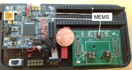
Most recent smartphones and tablets have inertial sensors integrated in their hardware. The three widely used types of inertial sensors are the gyroscope, the accelerometer and the magnetometer. Most embedded inertial sensors are MEMS (Microelectromechanical systems), notably known for their low consumption and volume. An example of MEMS sensors on a board can be seen on Figure 1-4. Other types of sensors are present such as pressure, light and proximity sensors. However, in the context of motion estimation they appeared less relevant. Each type of sensor possesses its own characteristics and they can be used directly or fused to perform a large range of applications. The fusion process consists in performing an estimation using measurements from multiple sensors types. This allows to overcome specific drawbacks from each sensor, even if some remain after using fusion techniques.
Figure 1-4: MEMs sensors on a board, with a 1 cent of Euro piece for scale. 1.3.2.1 Sensors characteristics
The gyroscope measures rotation speed in three dimensions. The measurement rate
ranges from 50Hz up to 500Hz. To obtain orientation information, it is necessary to integrate the data from the gyroscope, giving only a relative estimation on the rotation of the device from one measurement to the next. It leads to error accumulation, also known as drift, when measuring a biased sensor, which is always the case for MEMS gyroscopes. In our experiments, we noticed this type of sensor was the least noisy of the three, but as it only gives a relative estimation and it can drift, either fusion or specific filtering needs to be performed before using its measurements.
The accelerometer indicates the mobile acceleration that is composed of the gravity
and the mobile’s own acceleration. In the MEMS case, the sensor is usually very noisy. It is therefore very challenging to retrieve the true mobile acceleration from it, and even harder to estimate the speed or the position, as it requires integration of a highly noisy signal. Therefore the accelerometer is usually only used to deduce the direction of the gravity, providing an estimation of the mobile orientation without any integration needed. It must be considered that
19
making this assumption implies that the mobile’s own acceleration then becomes a form of noise.
The magnetometer estimates the earth magnetic field direction and so the magnetic
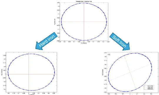
north. Similarly to the accelerometer, the measures are very noisy. In addition, magnetic perturbations add to the noise; the effects known as “soft iron” and “hard iron” lead to distortion in the local magnetic field. The hard iron is due to a magnetic reflection from an object, while the soft iron comes from interferences in the magnetic field, for instance due to a cellphone. Figure 1-5 displays an example of what a magnetometer measures when performing a 360° yaw rotation. We only represent the x and y axis, as the vertical axis does not vary. The upper graph shows the measurement without perturbations. The lower-left one displays the hard iron effect, and the lower-right one the effects of the soft iron. It can be seen that without any disturbances the north direction describes a round circle while the 360° turn is performed. However, in the presence of either soft or hard iron, the circle is either shifted (hard iron) or not round anymore (soft iron), which induces errors when estimating the north direction.
Figure 1-5: The effect of soft and hard iron on a magnetometer when performing a 360° turn. To sum up, each sensor has its own issues:
- The gyroscope provides a rotation speed estimation. Performing orientation estimation requires integration, which can create drift from biases.
- The accelerometer is very noisy, and as we want to estimate the gravity direction only, platform’s acceleration is to be added to noise.
- The magnetometer is also very noisy, and can undergo a lot of distortions due to various magnetic effects.
It is necessary to overcome those drawbacks by fusing the sensors to obtain a robust and accurate estimation of the orientation of the mobile.
20
1.3.2.2 Inertial sensors fusion techniques and applications
There are a lot of applications domains for inertial sensors fusion in embedded platforms, from Unmanned Aerial Vehicles (UAVs) navigation to Smartphone applications. For the Smartphones and Tablets the targets are mainly gaming, orientation awareness, pedestrian step counting, etc… The goal of inertial sensor fusion is to utilize the measurements from the three sensors simultaneously in order to compute the 3D orientation (and eventually position, even if it is highly challenging for low-cost sensors [Baldwin et al. 2007]) of the device. Two main techniques are utilized in the literature to accomplish this: the Kalman filter and the complementary filter.
The Kalman filter [Kalman 1960] is utilized in many domains and applications. It estimates over time a set of Gaussian unknown variables, called the state of the filter. The first two statistic moments are computed, that is the mean and the covariance of the state. This estimation is based on a physical model and measurement equations. Like most Bayesian filters, it proceeds in two steps: a prediction of the state of the filter and a correction of the prediction based on the measurements. The detailed operation of the Kalman filter is shown in Appendix A: The main requirement to apply it for inertial sensor fusion is to have an approximate knowledge of the noise model of every sensor. Usually, the biases of every sensor are explicitly computed in the state of the filter. One major limitation of the Kalman filter is that it can only estimate linear systems, both in terms of propagation and measurement. Therefore an extended version of it has been designed for non-linear systems: it linearizes locally the propagation and measurement equations. Many applications and adaptations of the filter, or its extended version, have been presented for inertial sensor fusion [Lefferts et al. 1982] [Julier & Uhlmann 1997] [Marins et al. 2003] [Kiriy & Buehler 2002] [Foxlin 1996].
The complementary filter is much more specific to inertial sensor fusion in terms of field of application. The sensors characteristics are taken into account in terms of their frequency performance for orientation estimation. On one hand, gyroscopes are quite accurate but suffer from drift as we need to integrate the measurements to compute orientation. Thus, they perform well to estimate high frequency motions, but poorly for low frequency ones. On the other hand, magnetometers and accelerometers possess heavy noise and perturbations, but their orientation measurements do not drift, as they respectively record the direction of the gravity and magnetic north. Therefore their performance is good in the low frequencies, but poor in the high frequencies. To maximize the potential of both sensors, the complementary filter has two steps: filtering every sensor output according to its frequency quality of estimation, and then combining the filtered signals. For instance, a low-pass filtering is performed on the accelerometer and magnetometer; a high-pass filtering is performed on the gyroscope; then the signals are combined. This type of filtering has been widely applied for inertial sensor fusion [Mahony et al. 2008; Mahony et al. 2005] [Euston et al. 2008] [Fux 2008]. The main advantage of this technique is its low-parameterization, as only cutoff frequencies are to be set. It can also be lighter in terms of computation processing than Kalman filtering.
21
1.4 Representation of a motion
As the study presented here is focused on motion estimation, a problem that arises is to adopt proper motion model representation. This will impact heavily some algorithmic and implementation choices and limitations. Firstly, the pinhole projective model is introduced, which is the classical model used for embedded video applications. In two dimensions, the problematic revolves around restrictions to the planar motion, going from a pure translation to perspective models, and even some more specific ones. In 3D the main concern is the type of rotation representations that can lead to singularities, difficulties in interpretation, and filtering problems.
1.4.1 Envisioning a 3D world with a 2D sensor
The pinhole camera model is the most applied in the computer vision domain. It describes the mathematical relationship between a 3D object viewed by the camera and its 2D projection on the image, as shown in Fig.1-1. It possesses many limitations: it does not take into account the focus of the camera which creates blur and it does not directly model the discretization that occurs when translating projected image into pixels. In addition, Image distortions due to lenses are not considered. However, this model is considered as a sufficient geometric approximation for many applications [Hartley & Zisserman 2003]. As one can see on fig. 1-1, the real final image plane presents a 180° rotation due to image rays crossing at the pinhole location. To simplify computation, a virtual image plane is often considered in front of the pinhole. All equations presented in this thesis will be based on this virtual image, which will now directly be referred to as the image to clarify and lighten the subject.
Figure 1-6: A pinhole camera model
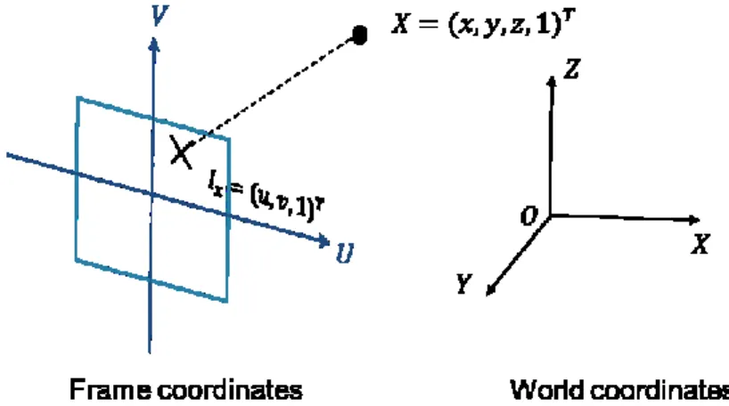
We now consider a point 𝑋 in 3D world homogenous (we add a 1 at the end of the classical coordinates to treat translation using multiplication) coordinates: 𝑋 = (𝑥, 𝑦, 𝑧, 1)𝑇. The
quantities 𝑥, 𝑦 and 𝑧 represent the world coordinates of the point. The image projection of the point 𝑋 is noted 𝐼𝑥 with its 2D pixel coordinates 𝐼𝑥 = (𝑢, 𝑣, 1)𝑇, 𝑢 and 𝑣 being the horizontal
22
and vertical pixel coordinates respectively. A scheme of this representation is displayed on fig. 2-2.
Figure 1-7: Coordinates notation
The pinhole camera model describes the relationship between 𝑋 and 𝐼𝑥. This is made in two
steps. Firstly, we need to explicitly model the geometric position and orientation of the camera with respect to world coordinates. This information is contained in a 3x4 projection matrix 𝑷 = [𝑹|𝒕], where 𝑅 is a 3x3 rotation matrix that encodes the orientation of the camera, and 𝑡 a column vector of 3 elements, representing the position of the pinhole center of the camera. Secondly, we need to explicit the transformation of the projection into pixel points. This is modeled by a camera matrix 𝑲. In some studies, 𝐾 is named the instrinsic matrix.
𝐾 = (
𝑓 0 𝑐𝑥 0 𝑓 𝑐𝑦 0 0 1
) (1)
where 𝑓 is the focal length of the camera, and (𝑐𝑥 , 𝑐𝑦)𝑇 the principal point of the camera, that
defines the projection of the camera principal rays into the image plane. Note that a square pixel is considered here, otherwise we would need to define two distinct focal length for the horizontal and vertical axis of the camera. The complete relationship between pixel location 𝐼𝑥and 3D coordinates 𝑋 is thus:
𝐼𝑥= 𝐾𝑃𝑋 (2)
While one may consider on-the-fly computation of both 𝐾 and 𝑃 matrices, in this study we considered that the camera matrix was computed once in a calibration process and then was considered fixed. The method of [Zhang 2000] was applied to every testing device used in the context of the thesis in order to compute the intrinsic camera matrix K.
1.4.2 In-plane motions
A 2D transformation between two frames can be expressed in many different manners. To keep the notation homogenous and simple, we will represent the transformation using the
23
coordinates’ changes of a point. A 2D homogenous point 𝐼𝑥 = (𝑢, 𝑣, 1)𝑇 in the first frame is
mapped to a point 𝐼′𝑥 = (𝑢′, 𝑣′, 1)𝑇 in the second frame by the transformation. Most of the
following descriptions for motion models is further described in the second chapter of [Hartley & Zisserman 2003].
The first type of motion that can be modeled is a direct translation 𝑇 = (𝑇𝑥, 𝑇𝑦). It has a very simple effect on the coordinates:
𝐼′𝑥 = ( 𝑢′ 𝑣′ 1 )=( 𝑢 +𝑇𝑥 𝑣 +𝑇𝑦 1 ) (3)
The main characteristic of this motion model is that it only has 2 degrees of freedom. Therefore it is computable from only one point correspondence from a local motion estimation technique or a global one such as integral projections [Crawford et al. 2004]. The limitation in terms of motion is very restrictive, and makes it only usable for very closely recorded frames. To our knowledge, the translational motion model has mainly been used for video encoding, where every block’s motion is estimated with a local translational motion model. This type of model can also be used in panorama and stabilization, if in-plane rotation is not considered.
Another type of 2D motion model is the rotation-preserving isometry, which correspond to an in-plane rotation by an angle 𝜃 combined with a translation:
𝐼′ 𝑥 = ( 𝑢′ 𝑣′ 1 ) =( cos(𝜃) − sin(𝜃) 𝑇𝑥 sin(𝜃) cos(𝜃) 𝑇𝑦 0 0 1 ) ( 𝑢 𝑣 1) (4)
Only one degree of freedom is added to the translation model, but as a point correspondence provides two pieces of data, two point correspondences are needed to compute the isometry. This motion model is widely used for video stabilization, providing translational and rotational movement estimation that can be filtered. It is also sometimes used in tracking applications, when the size of the object on the image is not expected to change during the sequence. For non-subsequent image motion estimation, scale changes need to be added to the motion model. This type of model is called a similarity transformation, with a scale change of 𝑍:
𝐼′ 𝑥 = ( 𝑢′ 𝑣′ 1 ) = ( Z cos(𝜃) −𝑍 sin(𝜃) 𝑇𝑥 Z sin(𝜃) 𝑍 cos(𝜃) 𝑇𝑦 0 0 1 ) ( 𝑢 𝑣 1) (5)
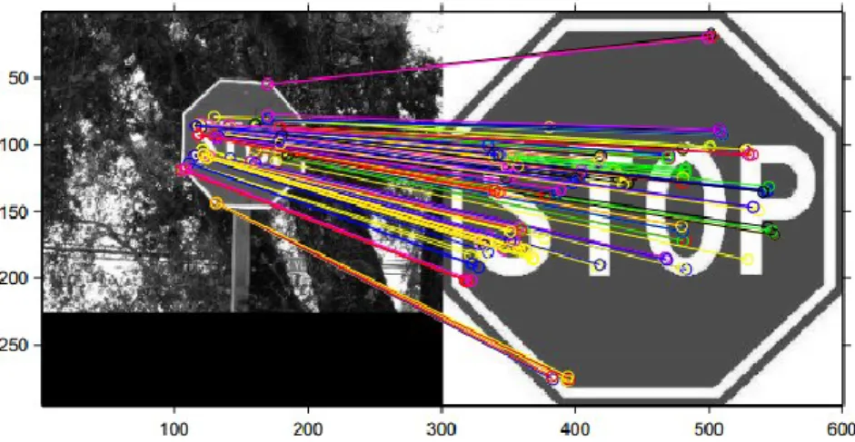
The augmentation of the model with scale opens up many application domains: long term tracking, recognition, etc… See fig. 2-7 for a recognition example based on local matching followed by a similarity motion model estimation. It can be seen that without the addition of the scale parameter, this recognition would have been impossible.
24
Figure 1-8: An example of similarity motion model applied to recognize a stop sign
Certain types of motions can lead to a deformation in the shape of the image. To include some simple transformations such as stretching or skewing we need to increase the number of parameters in the model:
𝐼′ 𝑥 = ( 𝑢′ 𝑣′ 1 )=( 𝑎11 𝑎12 𝑇𝑥 𝑎21 𝑎22 𝑇𝑦 0 0 1 ) ( 𝑢 𝑣 1) (6)
This type of representation is an affine transformation. For instance in [Auberger & Alibay 2014], this model is mapped to deduce specific deformations, created by motions recorded with a rolling shutter sensor. The extension to affine model was needed as these distortions do not preserve the shape of the image. As the degree of freedom is increased to 6, three points correspondences are needed to create this type of representation.
The last extension of this type of representation presented here is the projective transformation. The form of the transformation is the following:
𝐼′ 𝑥 = ( 𝑢′ 𝑣′ 𝑤′ )= ( 𝑎11 𝑎12 𝑎13 𝑎21 𝑎22 𝑎23 𝑎31 𝑎32 𝑎33) ( 𝑢 𝑣 1) (7)
Note than the third coordinate is modified in the final image point 𝐼′
𝑥. To retrieve the final
location of the point on the image, one should divide the coordinates of the point by 𝑤′. This model is needed when modeling “out-of-plane” transformations, for instance 3D rotations. It is useful in applications requiring the tracking of a planar structure moving freely in a scene. More complex 2D motion representations can be used, but their domain of application is more limited in the scope of this study.
1.4.3 Three dimensional representation of motions
3D motion representation is a complex subject. Many types of models exist, but only the most applied in our context of general motion estimation purposes will be displayed here. Rotation
25
representation will first be described. A discussion is made on how to combine it with translation. We here present the rotation matrix and Euler angles as they will be used in the thesis. Presentation of quaternions and exponential maps are presented in Appendix B:. 1.4.3.1 Rotation matrix
A rotation can be represented as a 3x3 matrix 𝑅. The matrix columns are each of unit length and mutually orthogonal, and the determinant of the matrix is +1. This type of matrices constitutes the SO(3) (for special orthogonal) group. Each matrix belonging to this group is a 3D rotation, and any composition of matrices from this group is a rotation. This representation of a rotation is the most direct one to apply, as a 3D point 𝑋 = (𝑥, 𝑦, 𝑧, 1)𝑇 is transformed by
𝑅 to a point 𝑋𝑟𝑜𝑡 = (𝑥𝑟𝑜𝑡, 𝑦𝑟𝑜𝑡, 𝑧𝑟𝑜𝑡, 1)𝑇 by a simple 4x4 matrix multiplication based on the
rotation 𝑅:
𝑋𝑟𝑜𝑡 = (𝑅 00 1)𝑋 (8)
It must be noted that most of the other rotations representations are converted to a rotation matrix to be applied. The main drawback of the rotation matrix is the complexity of the constraints to keep the matrix in the SO(3) group when applying optimization of filtering techniques. In effect, those techniques will modify the coefficients of the matrix, but it should always be orthonormalized to belong to the SO(3) group. This is done at heavy cost and needs to be performed at each step of the algorithm where the matrix is modified.
1.4.3.2 Euler angles
The Euler angles representation is the most used for 3D rotations. It consists in separating the rotations to a minimal 3 angle values that represent the respective rotations around the axis of the coordinates in a sequential way. They are referred to as the yaw, the pitch and the roll angles. According to the choice of the user, these three values are either expressed in degrees or radians. In order to apply the transformation to a point, the Euler angles are transformed into separate rotation matrices, which are combined to form the total rotation matrix that is then applied to the point. In this study, we will refer to the yaw as 𝛼, the pitch as 𝛽, and the roll as 𝛾. A big issue in using Euler angles is the necessity to establish a convention on the order of application of the angles. In effect, one can select which angle represents a rotation around an axis, as well as the order chosen to apply them. This can create confusion and misunderstandings. In fig. 2-8, one can see the axes displayed on a smartphone scheme. To specify the convention used in this study: the yaw is the rotation around the red axis, pitch around the green axis, and roll around the blue axis.
26
Figure 1-9: Smartphone with axis of superimposed. Image extracted from 4.
Another issue arising from Euler angles application is called the Gimbal lock. It happens when one Euler angle is equal to 90° (this can depend on the convention chosen), which leads to two axes of rotation becoming aligned, as displayed in fig1-10. This degenerate configuration induces a loss of one degree of freedom. Another issue with this representation is that it splits the rotation on the axis, it is difficult to interpolate and differentiate rotations, as it ignores relationship between the several directions.
Figure 1-10: Gimbal lock example. On the left, a regular configuration. On the right, one can see that two axes of rotation are aligned, decreasing the number of degrees of freedom. Image extracted from
Wikipedia5
1.4.3.3 Combination with translation
4http://www.legalsearchmarketing.com/mobile-apps/creating-a-mobile-app-for-your/ 5 https://fr.wikipedia.org/wiki/Blocage_de_cardan
27
A 3D motion is a combination of a rotation and a translation 𝜏 = [𝜏𝑥, 𝜏𝑦, 𝜏𝑧]𝑇. As seen
previously, one must always convert a rotation to a rotation matrix in order to apply it to a point. The complete motion regrouping a rotation 𝑅 and a translation 𝜏 is applied to a point 𝑋 by:
𝑋′ = (𝑅0 1𝜏)𝑋 (9)
As seen previously, many representations for 3D rotations can be used with various advantages and drawbacks. In SLAM systems, optimization or filtering techniques are applied to retrieve the 3D pose of a device. This often leads to the selection of Quaternion or exponential maps representations that show good properties for differentiation process and do not present disturbing singularities.
1.5 Structure of the thesis
Chapter 2 focuses on motion vector computation. An overview on local methods to compute motion is given, with a focus on feature-based procedures, and especially the ones with the less amount of computation needed. Additions on these techniques using inertial sensors are proposed, and then compared to non-hybrid techniques in terms of performance and computational cost.
In Chapter 3 the problem of computing the camera motion in two dimensions using visual and inertial measurements is studied. An overview of the state of the art techniques is made. Then, a real-time hybrid variation of the RANdom SAmple Consensus (RANSAC) method is proposed. Performance and computational resources are also studied.
Chapter 4 introduces the problem of hybrid localization, or visual-inertial odometry. With an overview on the state of the art techniques presented, hands-on experiments and discussions are made. A novel hybrid localization method is then proposed, which specificity relies on the numerous levels of fusion between visual and inertial measurements, in a very specific manner designed towards embedded platforms. Ground-truth based comparisons are made with state of the art methods, thanks to a setup based on infrared markers and cameras.
28
Chapitre 2: Calcul de point-clés
Below is a French summary of chapter2: Feature estimation.L’estimation d’une image à l’autre du mouvement de la caméra dans une séquence vidéo est un problème bien connu dans le monde de la vision par ordinateur. Dans une majorité de cas, la première étape de ces techniques est de calculer des vecteurs de mouvements entre deux images. Ceci est réalisé en mettant en correspondances des points d’une image à l’autre. Pour générer des vecteurs de mouvements, certaines méthodes procèdent à une extraction de points d’intérêts dans l’image, ou points-clés. Ceux-ci sont ensuite stockés sous forme de descripteurs, des représentations haut niveau du point qui sont en général construites afin d’être invariantes à certaines transformations : changement d’illumination, rotation du plan, flou… Nous proposons une amélioration d’un type de descripteur visuel, basée sur les mesures des capteurs inertiels.
Ce chapitre présente tout d’abord les différentes méthodes de génération de vecteurs de mouvements. Les descripteurs peu coûteux en temps de calcul sont étudiés de façon plus approfondie. L’extension inertielle apportée à ce type de descripteur est ensuite présentée. Finalement, une évaluation de ce nouveau système est présentée, avec des considérations sur l’efficacité calculatoire de notre approche.
30
Chapter 2: Feature estimation
Estimating the frame to frame camera motion in a video sequence is a highly studied problem. It is a key step in many applications: camera stabilization, rolling shutter distortions correction, encoding, tracking, image alignment for High Dynamic Range, denoising… The first step of this type of technique is generally to extract motion vectors between pairs of images. This is performed by putting in correspondences points from one frame to another.
Many factors can impact the performance of these methods. In a sequence, illumination changes can occur, modifying the pixels values from one frame to another. In-plane rotations create another dimension in the problem, which can no longer be solved as a 2D translation estimation. Motion artifacts, such as motion blur or rolling shutter distortions also intervene in the process, creating variation in terms of pixel values and localizations. Finally, scene characteristics can make a great impact on the results of those techniques: a lack of texture in the scene, low-light heavy noise, etc…
An overview of motion vectors generation methods is proposed in section 2.1 . A first category of algorithm makes use of pixel-wise computation. For a set of fixed given points in the first frame, a correspondence is searched in the second frame. This can be performed either for every point, which is generally called optical flow, or in a sparse manner, with techniques such as block matching or tracking. The second category of vector generation techniques consists in extracting points of interest in every frame that are also called keypoints, rather than using fixed points (or every point) in the frame. Descriptors of each set of points are then computed, which consist in a higher-level, more robust information on the surrounding of the keypoint. Correspondences are then drawn between these two sets of points, in an operation known as matching.
In section 2.2 , the focus is on a deeper look into light keypoint detection and description techniques. In the context of embedded platforms, it is suitable to spend as little resources as possible on the computation of motion vectors. Therefore, the focus of this thesis for feature estimation was centered on as light as possible methods.
A novel technique of light keypoint description extension with inertial sensors is described in section 2.3 . The main contribution in this scope is to study the possible impact of inertial sensors for description techniques, and to provide a valuable addition to binary descriptors. Robustness to geometric variations such as in-plane rotation or viewpoint changes is improved. With the global scheme of the method described, section 2.4 presents implementation and results of the process. Results show the improvement in robustness induced by the techniques. Implementation approximation is proposed to save as much computation as possible.
31 Finally, conclusions are drawn in section 2.5 .
2.1 From images to motion vectors
Two main methods exist to compute the motion vectors:
- Computing the position of a particular set of points from one frame to the next. It can be done in a dense manner (every point position is computed) or sparsely.
- Extracting points of interest in both frames, and intending to put them in correspondences, which is also called matching.
After performing the motion vectors computation, global camera motion is estimated with robust techniques. More recent techniques intend to combine the inertial measurements with the motion vectors to provide a robust and accurate estimation of the motion.
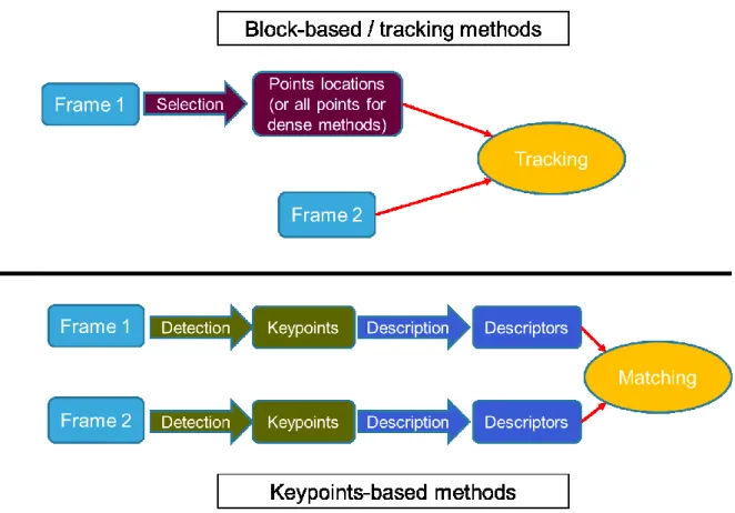
Figure 2-1: The two main types of motion vector computation techniques.
In Figure 2-1, one can see the two types of motion vector creation techniques. For block-based / tracking techniques, the first stage is selection of points: either considering points at a fixed location on the frame (with a grid pattern for instance), detecting keypoints, or every points for dense methods. Then the technique consists in finding the corresponding locations of the selected points in the second frame. For keypoints-based methods, keypoints are detected on every frame. Description algorithms are performed on the keypoints locations, creating descriptors, which are matched from one frame to another to generate motion vectors.
32
2.1.1 Block-based and global methods
While some techniques intend to find motion directly based on the whole image [Crawford et al. 2004], most of the recent techniques compute local motion vectors as a first step of a motion estimation procedure. A motion vector describes a mapping of a point in the previous frame to the current one. Block matching methods compute a difference function between two pixels based on their surroundings, which is a square area around each pixel called blocks. The main consideration in this type of algorithms is the number of candidates to test, as well as their locations. Differential methods intend to compute the motion for every pixel of the frame, by minimizing an energy that incorporates local and global terms [Horn & Schunck 1981]. 2.1.1.1 Block matching techniques
Block matching algorithms computes the similarity of two pixel blocks based on a difference function, either the Sum of Square Differences (SSD) or Sum of Absolute Differences (SAD). Then the motion vector computed is considered as an estimation of the motion of the center of the block. For a pixel point 𝑝 = [𝑢, 𝑣]𝑇 in the previous frame, we note its intensity 𝐼(𝑢, 𝑣). The
difference of this point 𝑝 with another point in the current frame 𝑝′ = [𝑢′, 𝑣′]𝑇 is computed
as 𝐷(𝑝, 𝑝′): 𝐷(𝑝, 𝑝′) = ∑ ∑ 𝑑𝑖𝑓𝑓(𝐼(𝑢 + 𝑖, 𝑣 + 𝑗) − 𝐼(𝑢′+ 𝑖, 𝑣′ + 𝑗)) 𝑗=𝑁 𝑗=−𝑁 𝑖=𝑁 𝑖=−𝑁 (10)
Where the function 𝑑𝑖𝑓𝑓 is either the absolute or square difference. This function 𝐷 is computed on a certain amount of locations, and the found minimum of the function is selected. The motion vector 𝑚𝑣(𝑝) = [𝑢′− 𝑢, 𝑣′ − 𝑣] is therefore created.
The SSD (or SAD) score presented can be used as a starting point in order to compute similarity between two points. However, it is not robust to illumination changes, neither to a shift nor to affine transformation. That is why a zero-normalized SSD score is preferable:
𝑍𝑁𝑆𝑆𝐷(𝑝, 𝑝′) = 1 (2𝑁 + 1)² ∑ ∑ ( 𝐼(𝑢 + 𝑖, 𝑣 + 𝑗) − 𝑚𝑝 𝜎𝑝 − 𝐼(𝑢′ + 𝑖, 𝑣′ + 𝑗) − 𝑚𝑝′ 𝜎𝑝′ )² 𝑗=𝑁 𝑗=−𝑁 𝑖=𝑁 𝑖=−𝑁 (11) Where 𝑚𝑝 and 𝑚𝑝′ are the mean values of pixel blocks around points 𝑝 and 𝑝′ respectively,
and 𝜎𝑝, 𝜎𝑝′ the standard deviation of those patches. While this technique is effective in order to compare points, it is not robust to rotations, scale, or viewpoints changes.
The key step of this method is to carefully choose the tested points in the previous frame. Many types of techniques exist to choose points, from spatial ones [Koga et al. 1981][Li et al.
33
1994][Po & Ma 1996][Zhu & Ma 2000], to spatial-temporal strategies [de Haan et al. 1993]. These methods were mainly developed towards video encoding.
2.1.1.2 Optical flow differential methods
Optical flow differential techniques intent to minimize the brightness constant constraint of the neighborhood around the pixels with derivate-based methods. Rather than only testing a few candidates, the Lucas Kanade Tracker (LKT) [Lucas & Kanade 1981] performs a gradient descent on the neighborhood around the point, inferring that the flow do not vary much in this location. A major improvement was proposed in [Bouguet 2001], that implements a pyramidal version of the tracker. It computes the gradient and optimizes the position on a reduced size image. This computed position is then taken as the starting point for the next image pyramid level, going from a very small image up to the real image size. Due to heavy cost of computation, adaptations have been made to port the algorithms on a graphical processor [Kim et al. 2009].
On another hand, the pioneer work of [Horn & Schunck 1981] displays an iterative method to compute the optical flow for every pixel, minimizing an energy term for each motion vector in both horizontal and vertical directions. This term relies on a combination of the brightness constancy constraint and the smoothness expected in the optical flow. A weighting value balances the importance between the smoothness and brightness constancy constraints. In a similar fashion to the LKT, the heavy computation cost has led to processing time reduction techniques [Bruhn et al. 2005].
The main difference between the two presented types of methods is that LKT strategy only relies on the neighborhood of a pixel, while Horn & Schunck variational methods add global constraints to the optical flow fields. In the literature, LKT is used when tracking a sparse set of points. When needing a dense field, variational methods are preferred.
2.1.2 Keypoints
The main drawback of previously presented methods for pixel motion estimation, is that every pixel does not carry the same amount of useful information. For instance, estimating the motion of a white point on a white wall is much more challenging than a black point on the same wall. If a motion needs to be estimated from two images that present changes in terms of conditions and location, we need robustness to various transformations in our estimation approach: illumination changes, rotation, scale… Approaches of feature extraction have been designed with the goal of finding locations in the images that carry most information and distinctiveness. Many types of features exist, including points, blobs, edges… In this study we restricted our interest to points and blobs that are present in most types of sequences which makes them suitable for embedded applications. These points of interest are called keypoints.
34
An overview of feature detection strategies is presented, followed by feature description techniques. Then a short discussion is made about matching vs. tracking strategies. Finally, an overview of existing hybrid methods for keypoints computation is done.
2.1.2.1 Detection: From corners to Local extrema detection
One of the first works done in keypoint detection has been demonstrated in [Moravec 1980] which served as base for the Harris corner detector [Harris & Stephens 1988]. It is based on an auto-correlation function 𝑎 of a point 𝑝 = [𝑢, 𝑣]𝑇 and a shift [Δ𝑢, Δ𝑣]𝑇 :
𝑎(𝑝, Δ𝑢, Δ𝑣) = ∑ ∑ (𝐼(𝑢 + 𝑖, 𝑣 + 𝑗) − 𝐼(𝑢 + Δ𝑢 + 𝑖, 𝑣 + Δ𝑣 + 𝑗))² 𝑗=𝑁 𝑗=−𝑁 𝑖=𝑁 𝑖=−𝑁 (12)
If this auto-correlation is small in every direction, this translates a uniform region with little interest. Only a strong value in one direction most likely indicates a contour. If every direction displays strong values however, the point is considered a keypoint. With a first-order Taylor approximate, the auto-correlation matrix can be expressed in function of spatial derivate of the image. The keypoint evaluation is then made with regard to the eigenvalues 𝜆1, 𝜆2 of that
matrix. The corner-ness function is:
𝑓(𝑝) = 𝑑𝑒𝑡(𝑎(𝑝)) − 𝑘(𝑡𝑟𝑎𝑐𝑒(𝑎(𝑝)))2 = 𝜆1𝜆2− 𝑘(𝜆1+ 𝜆2)² (13) If this value at pixel 𝑝 is higher than a threshold and higher than cornerness function 𝑓 evaluated on neighborhood points, the point is considered a corner. The threshold can be set in function of the total desired number 𝑁𝑐𝑜𝑟𝑛𝑒𝑟𝑠 of corners, or an absolute quality desired. The fact that the
detectors consider all directions of a gradient matrix induces its robustness to illumination changes as well as in-plane rotations. Other methods have been designed based on the gradient matrix to detect corners [Förstner 1994], some extending the Harris detector to make it scale invariant [Mikolajczyk & Schmid 2001]. [Rosten & Drummond 2006; Rosten et al. 2010] presented Features from Accelerated Segment Test (FAST), a very light extractor in terms of computational time that will be further described in section 2.2.1 . The FAST keypoint extractor is based on a number of continuous pixels on a circle with a marked difference with the center. Several detectors have been developed to cope with scale invariance. They consist in searching the scale-space dimensions of the image and finding the extremas of an operator, which can be the gradient, Laplacian, etc… The image is first convolved by a Gaussian Kernel to smooth noise. Values are then normalized with respect to scale, and a point that possesses the highest absolute value of the neighborhood is then considered an interest blob (a keypoint with higher scale than just a pixel). The Laplacian has been demonstrated to be the best operator to choose [Lindeberg 1998].
35
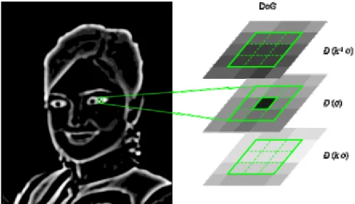
In this context, the SIFT detector is presented in the work of [Lowe 2004], making use of the difference of Gaussians approach between scales. On Figure 2-2, an example can be seen of a feature detected in a difference of Gaussians image. For every scale, the Laplacian operator is approximated by a difference between two Gaussians smoothed images with different values for Gaussian smoothing. Maxima / minima are then detected by comparing every point with its direct neighborhood in the space scale dimensions, reducing the number of comparisons needed to only 26 neighbors.
Figure 2-2: Scale space detection based on difference of Gaussian, extracted from 6.
To speed-up processing, [Bay, Tuytelaars 2006] presented SURF, a method based on the Hessian matrix of a point 𝑝 at scale 𝜎:
𝐻(𝑝, 𝜎) = (𝐼𝐼𝑥𝑥(𝑝, 𝜎) 𝐼𝑥𝑦(𝑝, 𝜎)
𝑥𝑦(𝑝, 𝜎) 𝐼𝑦𝑦(𝑝, 𝜎)) (14)
Where 𝐼𝑥𝑥(𝑝, 𝜎), 𝐼𝑥𝑦(𝑝, 𝜎), 𝐼𝑦𝑦(𝑝, 𝜎) are the second-order derivate of the image in their
respective directions. The value used to perform blob detection is the determinant of the Hessian matrix. A non-maxima suppression by comparison of the neighborhood in the space scale dimensions is then performed, in a similar fashion to the SIFT method. SURF was mainly developed to propose a less expensive alternative to SIFT, using approximations to perform similar treatments. Mixed techniques also exist, using different operators to compute the scale and space selections [Mikolajczyk 2004].
To increase robustness to viewpoint changes, affine-invariant detectors were developed, using second moment matrix to estimate affine neighborhood [Lindeberg 1998], before applying it to the scale invariant blobs [Mikolajczyk & Schmid 2002]. Other techniques apply a connected components strategy in thresholded images in order to detect blobs [Matas et al. 2004]. While showing excellent results in terms of repeatability and robustness to viewpoint changes, these detectors have been measured as prohibitively expensive for real-time
36
applications in multiple comparisons [Mikolajczyk et al. 2005] [Moreels & Perona 2007] [Gauglitz et al. 2011].
2.1.2.2 Feature description
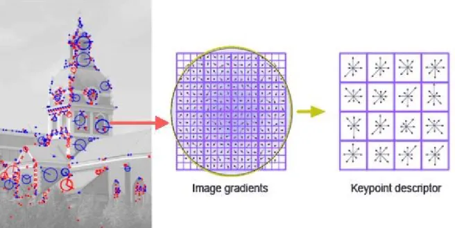
In the same efforts to improve detection robustness, keypoints descriptors techniques were developed to provide invariant representation of the surroundings of the desired area. Early techniques have been presented in order to deal with this issue [Freeman & Adelson 1991] [Schmid & Mohr 1997], but the SIFT descriptor [Lowe 2004] was the first widely used robust keypoint descriptor. The descriptor is based on the scale extracted from the keypoint (see previous section). It determines a dominant rotation in the scaled patch around the point. Image gradients are then computed in zones, and a soft assignment is made to map them into 8 discrete orientations (see Figure 2-3). The normalized histogram of gradients strength into each direction for every spatial zone constitutes the descriptor. It is a 128-dimensional vector of continuous numbers: 4x4 spatial zones times 8 orientations. To compute the similarity between two SIFT descriptors, one simply has to compute the L2-norm between them.
Figure 2-3: Feature description with SIFT, courtesy of 7.
SIFT is still a widely used descriptor, its main drawback being that the L2-norm between two 128-dimensional vectors can become very expensive to compute, especially when computing similarities between many points. [Ke & Sukthankar 2004] and [Mikolajczyk & Schmid 2005] introduced Principal Component Analysis (PCA) methods to reduce the dimension of the vector, decreasing the computation of matching. In the same spirit than extractors, [Bay, Tuytelaars 2006] presented approximations by box filtering of the description with SURF. Taking into account the computer quickness in computing the binary Hamming distance (just a XOR operation followed by a bit count), recent techniques were developed to produce binary
37
descriptors. Binary Robust Independent Element Features (BRIEF) [Calonder et al. 2010] utilizes pairwise comparisons along a determined pattern to build the binary string descriptor. The pattern is built with a random generation technique based on a Gaussian sampling that has been proven superior against other sampling strategies [Calonder et al. 2010]. This descriptor will be further described in section 2.2.2 . As BRIEF is not robust to scale or rotation changes, it is mostly used for video sequences needing frame to frame matching. To circumvent this, propositions have been made to bring invariance to rotation and scale to the detector with ORB [Rublee et al. 2011] and BRISK [Leutenegger et al. 2011]. Other methods used a regular pattern to perform the comparisons either for dense matching purposes [Tola et al. 2010], to avoid sampling effect [Leutenegger et al. 2011] or to approach the computation to human retina interpretation [Alahi et al. 2012].
The following table summarizes the invariances of some descriptors presented: Technique In-plane rotation Scale invariant Perspective invariance Computational cost Matching norm used SIFT ++ ++ + -- L2 SURF ++ ++ + - L2 BRIEF - -- - ++ Hamming ORB ++ -- - + Hamming BRISK ++ ++ - + Hamming
Table 1: Summary of the performance of some keypoint descriptors. ++ indicates strong performance in the considered category, down to – for inefficiency.
2.1.2.3 Methods using hybrid keypoints
To further improve robustness to rotation of the descriptors, [Kurz & Ben Himane 2011] proposed a gravity oriented version of SIFT. Rather than performing a visual technique to extract the dominant orientation of the patch, the readings of an accelerometer are used. This allows further discrepancy of the patch to transformations, as well as slightly reducing the computational cost. In Figure 2-4, one can see the benefit of orientating the descriptor with respect to gravity on a synthetic example. On the left, one can see that with visual information only, every window’s corner would have been described similarly along the dominant gradient. With the addition of gravity direction on the right, their descriptors are effectively modified, allowing to distinguish one from another. In further work [Kurz & Benhimane 2011; Kurz & Benhimane 2012] the utility of gravity oriented features has been demonstrated for more specific augmented reality applications.
38
Figure 2-4: Gravity benefit on keypoint discrepancy, extracted from [Kurz & Ben Himane 2011]
[Hwangbo et al. 2009] directly apply the gyroscopes readings in order to change the window of research of the LKT algorithm. With the yaw and pitch measurements they pre-set a translation value to the research window of every point, while the roll is applied to rotate it. This makes the LKT much more robust to quick motions.
2.1.2.4 Keypoint state of the art: discussion
As seen in the various techniques developed in the literature, inertial sensors bring an information on the orientation of the smartphone that is used to increase robustness to geometric transformations. They can also be used to predict the motion of the platform to adapt the search window of a technique. However, they do not bring any valuable addition to scale computation of a keypoint, which can only be computed from visual sensor recordings. As this study targets real-time performance for applications with high frame rate (up to 60 fps on modern smartphones) and resolution, an emphasis on low-cost technique selection has been stated. The addition of inertial sensors has been proven efficient for classical descriptors such as SIFT [Kurz & Ben Himane 2011], or heavy tracking strategies such as the LKT [Hwangbo et al. 2009].
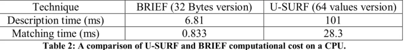
To provide maximum efficiency of computation, we decided to utilize binary descriptors and light detectors (such as FAST) for the applications developed in this thesis. An example of processing time comparison between classical descriptors such as Upright SURF (U-SURF), which is a non-rotational invariant variation of SURF, and BRIEF is provided in [Calonder et al. 2012]: