HAL Id: hal-01583283
https://hal.archives-ouvertes.fr/hal-01583283
Submitted on 7 Sep 2017
HAL is a multi-disciplinary open access archive for the deposit and dissemination of sci-entific research documents, whether they are pub-lished or not. The documents may come from teaching and research institutions in France or abroad, or from public or private research centers.
L’archive ouverte pluridisciplinaire HAL, est destinée au dépôt et à la diffusion de documents scientifiques de niveau recherche, publiés ou non, émanant des établissements d’enseignement et de recherche français ou étrangers, des laboratoires publics ou privés.
Optimal Embedded Sensor Placement for Spatial
Variability Assessment of Stationary Random Fields
Franck Schoefs, Emilio Bastidas-Arteaga, Trung-Viet Tran
To cite this version:
Franck Schoefs, Emilio Bastidas-Arteaga, Trung-Viet Tran. Optimal Embedded Sensor Placement for Spatial Variability Assessment of Stationary Random Fields. Engineering Structures, Elsevier, 2017, �10.1016/j.engstruct.2017.08.070�. �hal-01583283�
Please cite this paper as:
Schoefs F, Bastidas-Arteaga E, Tran T-V. (2017). Optimal Embedded Sensor Placement for Spatial Variability Assessment of Stationary Random Fields. Engineering Structures
https://doi.org/10.1016/j.engstruct.2017.08.070
Optimal Embedded Sensor Placement for Spatial Variability Assessment of
Stationary Random Fields
Franck Schoefs1, Emilio Bastidas-Arteaga1,†, Trung-Viet Tran1
Université Bretagne Loire, Université de Nantes, GeM, Institute for Research in Civil and Mechanical Engineering, CNRS UMR 6183, Nantes, France
ABSTRACT
Structural reliability assessment is largely influenced by the spatial variability of material properties or defaults; however, there are still various challenges for their characterization and modeling. Structural Health Monitoring (SHM) could provide useful information in space and time for spatial variability characterization of material properties and mechanical solicitations; nevertheless, this challenge is arduous because of the large number of potential sensor positions of local disruptions/failures. This paper proposes a methodology to optimize the spatial distribution of embedded sensors used for spatial variability assessment of stationary random fields. The optimization criterion relies on the width of the confidence interval of statistics for the characteristics to identify. For sake of simplicity, the paper illustrates the method for one-dimensional problems. The proposed method is applied firstly to a numerical example were several hypothetical structural configurations that could be found in practice are studied. It is finally applied to two case studies (a reinforced concrete beam and a steel wharf) where water content and loss of steel thickness are respectively measured. The results show that the stationary property is useful to deduce the minimum quantity of sensors and their position for a given quality requirement. They also allow us to propose a criterion for defining if regular or non-regular spacing of sensors along the inspection zone is more appropriate depending on the component length and autocorrelation structure of the random field.
Keywords: spatial variability; confidence interval; inspection optimization; stationary field; Karhunen-Loève expansion; sensor spacing; Structural Health Monitoring.
1. INTRODUCTION
Structural serviceability and safety are influenced by the different sources of uncertainty involved during their whole lifetime: material properties, loading, measures, model, deterioration, etc. A probabilistic structural analysis that includes the more influential uncertainties is therefore paramount to minimize both failure risks and design and maintenance costs. Nowadays, there are significant advances in probabilistic modeling at the scale of a single section of the structure. However, various works have demonstrated that the reliability assessment for a given component is largely influenced by the spatial variability of material properties or defaults [1–7]. Although the consideration of spatial variability is essential for proper reliability assessment, there are still various challenges for their characterization and modeling.
Non-Destructive Testing (NDT) and Structural Health Monitoring (SHM) could provide useful information in space and time for spatial variability characterization of material properties and mechanical solicitations. Several studies focused on the use of NDTs for spatial variability characterization at a given time. For example, Nguyen et al [8,9] combined several NDT techniques, kriging and variograms to assess the spatial variability of concrete at different scales (point, local and global). Gomez-Cardenas et al. [10] proposed a two-step approach to optimize the number and position of ultrasound measures required to localize critical zones. More recently, Schoefs et al. [11] proposed a methodology to find an optimal inspection configuration (number and localization of NDT measures) that
†corresponding author: tel: +33 2 51 12 55 24, email: [email protected], Address: 2 Rue de la
2 minimizes the error of identification of probability distributions for a given quantity of interest (resistance, porosity, water content, etc.) with spatial dependency. When an adaptive procedure can be selected on site for NDT, SHM requires a predefined design of embedded sensors positions. The main advantage of SHM relies on its capability to characterize the evolution in time of this spatial variability. Most part of research efforts in SHM have focused on the spatial localization of defects or damage of structural components [12–14]. However, spatial variability characterization of loading or material properties from SHM data is still a challenge because of the finite number of sensors and the large number of potential positions of local failures or disruptions. Numerical algorithms and specific multi-sensor systems should be developed towards this aim.
Within this framework, the main objective of this paper is to propose a methodology to optimize the spatial distribution of embedded sensors used for spatial variability assessment of stationary random fields. Stationary random fields have a stochastic structure and probabilistic properties that could be used to provide rational aid tools for optimizing the number and location of sensors. The paper shows that the stationary property of random fields is sufficient to achieve the optimal quantity of sensors and their position in view to provide a realistic characterization. The assessment of the shape of the Auto-Correlation Function (ACF) is paramount for spatial variability characterization. It is also essential to provide optimal measure positions for NDTs during inspection campaigns [11,15]. With respect to our previous work of focusing on NDTs [11], the main advantage of using embedded sensors for spatial variability characterization is that the stochastic properties are less sensitive to environmental conditions (sun, humidity, temperature, etc.) in depth leading to better assessment. Stochastic properties could also vary with time (e.g. for deterioration processes [16–18]); however, the evolution of spatial variability with time is beyond the scope of the present paper. In addition, since previous studies have shown that non-regular spacing of sensors is more efficient for identification purposes [19], non-non-regular sensor distributions will be considered in this study as a factor of optimization.
The paper starts in section 2 with a review of key concepts of spatial random field modeling with a focus on stationary random fields. Section 3 describes the proposed method for optimal sensors positioning in order to characterize the spatial correlation structure. This proposed strategy is illustrated with numerical examples (section 4) and real measurements on a reinforced concrete (RC) beam and a steel sheet-pile (section 5).
2. SPATIAL RANDOM FIELD MODELING
Random field theory provides a useful tool for spatial variability modeling. Among the different random field, a stationary stochastic process has been used in several applications [4–6,20–28] to represent spatial variability when the random field is considered homogeneous (symmetric field). These examples consider generally 1D stochastic processes. If 2D or 3D study cases are under consideration, the number of parameters to be identified increases (see section 2.3) but the methodology remains the same. This section summarizes the main assumptions and methods for stochastic modeling considered in this study. See [11] for more details.
2.1. Main assumptions for the stochastic modeling
In order to simplify the presentation of the proposed methodology, we consider the following main assumptions about the sensors and the random field modeling:
• The stochastic field is considered as: Gaussian, second order stationary, statistically homogeneous and its marginal distribution is known. This assumption implies that less information is required for its characterization.
• Each realization (single trajectory) represents the probabilistic information of all trajectories: mean, variance, spatial correlation. A single trajectory is then sufficient to describe the spatial variability, i.e. the stationary field is ergodic.
• A larger number of discrete sensors can be placed over the same component to characterize both randomness and spatial variability (e.g., from 20 to 60).
• Sensor measurements are considered as ‘perfect’ [15]. That means that (i) there is no bias and (ii) the error is insignificant or repetitive tests allow obtaining a good estimate of the real value and therefore to neglect the error. Nevertheless, if the error of the measure is well characterized, it could be also included in the analysis. This assumption helps to compute the inherent potential of the methodology and is consistent if the uncertainty on measurement is low. If it not the case, that will affects the estimation of the autocorrelation parameters and will lead to bad decisions with specific estimators. This aspect is beyond the scope of the paper.
2.2. Karhunen-Loève expansion
Given a probabilistic space (Ω, ℱ, P), a stochastic field or process with time or space is a collection of valued random variables indexed respectively by a set x “space” or t “time”. Let us denote Z(x,) the one-dimensional stochastic field, where represents the randomness and x the spatial coordinate. Z(x,i) is
called the ith sample function (or trajectory) of this field and corresponds to a given realization i of the
field for whatever location. Z(x1,) is a random variable that is generated by at a given location x = x1.
Since we consider here only homogeneous random fields, the marginal distribution of Z(x1,) does not
depend on the location.
This paper uses a Karhunen-Loève expansion to model the stochastic field Z(x,) [29]. This expansion represents a random field as a combination of orthogonal functions on a bounded interval [–a, a]:
𝑍(𝑥, 𝜃) = 𝜇𝑍+ 𝜎𝑍∑ 𝜉𝑖(𝜃)
𝑛𝐾𝐿
𝑖=1
√𝜆𝑖𝑓𝑖(𝑥) (1)
where μZ is the mean of the field Z, σZ is the standard deviation of the statistically homogeneous field Z,
nKL is number of terms in the expansion, i is a set of centered Gaussian random variables and i and fi
are, respectively, the eigenvalues and eigenfunctions that depend on the type of ACF ρ(Δx). It is possible to analytically determine the eigenvalues i and eigenfunctions fi for some correlation functions (see [11]
or [30] for more details). For example, for an exponential ACF [31]: 𝜌(Δ𝑥) = 𝑒𝑥𝑝 (−Δ𝑥
𝑏 ) , 0 < 𝑏 and Δ𝑥 = 𝑥1− 𝑥2 (2)
where b is an autocorrelation parameter and Δx [–a, a]. The spatial variability of various material properties or model parameters could be represented by an exponential autocorrelation. For instance, Jaksa et al. [26] used an exponential ACF to represent the spatial autocorrelation of the measurements from cone penetration tests measurements in Australia and other authors also recommend this model ([5,11]). Figure 1 illustrates how the exponential ACF provides a good fitting, according to Maximum Likelihood Estimate (see section 3.4), for representing the spatial variability of water content in a RC beam and corrosion in a steel sheet-pile. Generally speaking, the selection of the best ACF to represent the spatial variability depends on the intrinsic characteristics of the studied phenomenon. For simplicity, this study assumes that the random fields of the studied applications follow exponential ACFs. In case of homogeneous 2D or 3D random fields, equation (1) contains y and z coordinates with a unique value b to be identified. In case of non-homogeneous random fields, other parameters bx, by, bz in the 3D case will
be estimated.
3. SENSOR PLACEMENT STRATEGY AND GOALS 3.1. Key ideas for sensor placement
The paper focuses on the assessment of the ACF of a stationary field. An optimal geo-positioning of sensors along a trajectory (sampling of the random field) (Figure 2-up) should provide an accurate assessment of the ACF parameters (i.e. b in eq. (2)) with a limited number of sensors. When looking for the usual shape of a correlation function (Figure 2-down) a regular spacing of sensors could not be optimal. If the distance between two sensors Lb is large the decay of autocorrelation for short distances
cannot be assessed (e.g., 0m<distance<5m in Figure 2-down). On the contrary, if Lb is small, there is
some information provided for many sensors that will not be useful for the assessment of b (e.g., distance>5m in Figure 2-down). Figure 2 shows that it is possible to install different number of sensors for high and low autocorrelation zones to obtain a good assessment of the autocorrelation parameter by reducing the total number of sensors Ns. The objective is to get a spacing of sensors providing a larger
amount of data in the zone of high correlation. However, there is a limited feedback on the autocorrelation function (and consequently the value of b) for defining clearly the high autocorrelation zones. Section 4 presents a sensitivity study about the influence of the a priori knowledge of b. The following subsections describe the proposed procedure for determining the non-homogeneous spatial distribution of sensors.
3.2. Definition of the Spatial Correlation Threshold (SCT)
This paper considers a one-dimensional spatial field. The methodology could be applied on a set of trajectories representing: (i) a set of 1D components (beams), or (ii) a very long 1D-component
4 subdivided artificially or physically (expansion joint or construction joints) in a set of short components, or belonging to a wall structure (steel sheet pile or concrete wall).
In order to limit monitoring costs (number of sensors), we propose to monitor some zones of a trajectory with sensors separated by “sufficiently short distance Lb” allowing us to assess the shape of the
ACF (eq. (2)) that is controlled by the parameter b. This “sufficiently short distance” can be seen as an Inspection Distance Threshold (IDT). Thus the non-regular distances of sensors spacing 𝐿𝑏𝑖 should satisfy:
𝐿𝑏𝑖 ∈ ]0, IDT[ in the highly correlated zones.
The IDT is defined by assuming that, after a given distance, the events measured from an inspection can be assumed as weakly correlated. A Spatial Correlation Threshold (SCT) defines this weak correlation. For instance, Schoefs et al. [11] proposed a value SCT = 0.3 to get fairly correlated events and SCT = 0.5 to get high correlated events. For an exponential ACF, the SCT is linked with IDT by:
IDT = −𝑏 ∙ 𝑙𝑛(SCT) (3)
It was shown in [32] that a statistical error on the estimation of b can occur when limited measurements are available. Between the two values 0.4 and 0.5 and to increase the chance to get correlated values, this paper considers the value SCT = 0.4 to determine IDT. For example, for this value of SCT and b = 1.0 m, IDT = 0.92 m. The effect of this choice is discussed in [11].
3.3. Parameterization of the non-regular spacing
In view to reduce the set of potential solutions and simplify the design of the network of sensors, we propose a parameterization. It is based on a division of the trajectory (structural component) into np
segments of same size Lm (see Figure 2) and then a subdivision of each segment into a decreasing 𝑁𝑐𝑖
number of equidistant sensors, with distance 𝐿𝑖𝑏, following a series according to the octree approach. This
approach has the advantage to get more information (more sensors) for small distances between points where the slope of the auto-correlation function must be fitted accurately. The number of sensors in the first segment is computed by:
𝑁𝑐1= Round ( 𝑁𝑠 1 + ∑ 1 2(𝑖−1) 𝑛𝑝 𝑖=2 ) (4)
The number of sensors for the segments 𝑁𝑐2, … , 𝑁𝑐 𝑛𝑝−1
(i.e., 𝑁𝑐𝑖 with i ∈ [2;np–1]) is estimated from:
𝑁𝑐𝑖= Round ( 𝑁𝑐1
2(𝑖 − 1)) (5)
Since 𝑁𝑐𝑖 should verify 𝑁𝑠= ∑ 𝑁𝑐𝑖 𝑛𝑝
𝑖=1 , the number of sensors for the last segment, 𝑁𝑐 𝑛𝑝
, is the remaining number of sensors:
𝑁𝑐𝑛𝑝 = 𝑁
𝑠− ∑ 𝑁𝑐𝑖 𝑛𝑝−1
𝑖=1
(6)
The only necessary inputs are the number of sensors Ns and the number of segments np. The
distribution of sensors per segment is computed from equations (4) to (6). For instance, for 3 segments and 23 sensors, 13 sensors are placed in the first segment, 7 sensors in the second and 3 sensors in the last one. Figure 2 presents the distribution of sensors for this case.
Knowing the number of sensors in each segment, the distance between sensors in each segment is deduced as follows: 𝐿𝑖𝑏= { 𝐿 𝑛𝑝(𝑁𝑐1− 1) , if 𝑖 = 1 𝐿 𝑛𝑝𝑁𝑐𝑖 , otherwise (7)
To satisfy the condition of sufficient correlation between measurements (section 3.2), we should avoid a distance larger than IDT for the segments located in the high correlation zone (Figure 2). The length of this zone Lhc depends on the autocorrelation parameter b and could be estimated from eq. (2) by
𝐿𝑏𝑖 > 𝐼𝐷𝑇 for the segments located in this high correlation zone, the total number of sensors, N
s, should
be increased until ensuring this condition for a given number of segments.
This discretization technique fixes a deterministic shape of the sensor distribution with a given non-regular distribution of the lag. The objective now will be to optimize the number and position of sensors (number of segments) in view to reach a given quality on the estimation of the parameter of the ACF.
3.4. Parameter estimation, sensitivity analysis and optimization
Stationary stochastic fields are simulated by the Karhunen-Loève expansion (eq. (1)) assuming an exponential ACF (eq. (2)), whose parameter b has to be identified by knowing the two first statistic moments (𝜇𝑍, 𝜎𝑍). Based on a continuous trajectory, for fixed values of Ns and np, we obtain a sample of
discrete realizations from the sensor measurements 𝑍̂ = {𝑧1, 𝑧2, … , 𝑧𝑁𝑠} corresponding to the sensors
positions 𝑋 = {𝑥1, 𝑥2, … , 𝑥𝑁𝑠} following the discretization procedure presented in section 3.3. Discrete values of the auto-correlation function are deduced from 𝑍̂ and given by [25]:
𝜌𝑘=∑ (𝑧𝑖− 𝜇𝑍)(𝑧𝑖+𝑘− 𝜇𝑍)
𝑁𝑠−𝑘
𝑖=1
∑𝑁𝑖=1𝑠 (𝑧𝑖−𝜇𝑍)²
, 𝑤𝑖𝑡ℎ 0 ≤ 𝑘 ≤ 𝑁𝑠 (8)
We assess the value of b by using the Maximum Likelihood Estimate method (MLE), reported by Li [3]. The principle of the method is to find the best parameter (i.e. b in eq. (2)) for a given ACF candidate that gives the best fit to the experimental autocorrelation (eq. (10)) with respect to MLE estimate. This last one is better that the least square method that can lead to a biased estimation when data are lacking. The MLE for the estimation of b is computed by following the steps described by Kenshel [33] from:
𝐿ℎ= ∏ ( 1 √2𝜋𝑒𝑥𝑝 ( −𝑣𝑖2 2 )) 𝑁𝑠 𝑖=1 = ( 1 √2𝜋) 𝑁𝑠 𝑒𝑥𝑝 (− ∑ 𝑣𝑖 2 𝑁𝑠 𝑖=1 2 ) (9)
where i is the ith component of the vector of independent standard values obtained from:
𝒗 = C−1(𝑍̂ − 𝜇𝑍̂
𝜎𝑍̂ ) (10)
where 𝑍 ̂ is the vector of realizations of the random variable Z from sensor measurements and C a lower triangular matrix such that CCT= ρ and ρ the auto-correlation matrix. Besides, maximize L
h is equivalent to minimize L1: 𝐿1= ∑ 𝑣𝑖2 𝑁𝑠 𝑖=1 (11) The estimated parameter of the auto-correlation function, 𝑏̂ , is then obtained by solving:
𝑏̂ = arg 𝑚𝑖𝑛 𝑏∈𝑅+ ∑ 𝑣𝑖 2 𝑁𝑠 𝑖=1 (12)
To account for the effect of random shape of trajectories, the analysis is carried out over a database containing 10,000 trajectories generated by Monte-Carlo simulations. This allows estimating 10,000 values 𝑏̂ for each distribution of the sensor – i.e. one set of the couple (Ns, np). Note that in case of non
homogeneous random fields, other parameters bx, by, bz in the 3D case, will be estimated from equation
(12).
We select in this paper a confidence interval of the mean 𝜇𝑏̂ expressed as a percentage Δ of the theoretical (true) value bth to evaluate the quality of the SHM. From the 10,000 Monte-Carlo simulations
we estimate the bounds of the confidence interval and the probability 𝑃𝐼,𝑏 to get values inside the
confidence interval, from the monitoring data. In a reliability study, 𝑃𝐼,𝑏 will be discussed according to the requirements on the accuracy of the probability of failure assessment [23]. Thus we focus on the quality estimator:
𝑃𝐼,𝑏= 𝑃(𝜇𝑏̂∈ [(1 − Δ)𝑏𝑡ℎ, (1 + Δ)𝑏𝑡ℎ]) (13)
6 𝜇𝑏̂= 1 10,000 ∑ 𝑏̂𝑘 10,000 𝑘=1 (14)
We define another estimate εb, the normalized quadratic error of the parameter 𝑏̂:
𝜀𝑏 = (
𝑏̂ − 𝑏𝑡ℎ
𝑏𝑡ℎ ) 2
(15) Note that 𝑃𝐼,𝑏 is sensitive to Ns, np and the ratio IDT/L (Eqs. (6)-(10)). We analyze in the following
this sensitivity by varying the number of sensors (Ns), the number of segments (np) and the ratio IDT/L.
Finally, the optimal position and number 𝑛𝑝𝑜𝑝𝑡 of sensors is obtained by: 𝑛𝑝𝑜𝑝𝑡= 𝐴𝑟𝑔max
𝑛𝑝
{𝑃𝐼,𝑏(𝑁𝑠)} (16)
A numerical application will be presented in the next section to illustrate this sensitivity analysis.
4. APPLICATION TO A NUMERICAL STUDY CASE 4.1. Reference case: presentation, results and discussions
For illustrating the methodology and generalization purposes, it is considered in the following sections a set of 1D-components (beams) with a very large total length L>>b. The case of components with a limited size is discussed in section 4.2, excepting those where L < Lb for which it is theoretically impossible to
identify fully the stochastic field. The Gaussian stationary stochastic field is characterized by: the theoretical auto-correlation parameter bth=1m, IDT=0.92m from eq. (3),
Z = 100 and σZ = 20. The
objective is to optimize the position of sensors in view to reach a good assessment of the auto-correlation parameter b for an error Δ = 10%.
We first analyze the effect of the number of segments (np) on the quality of assessment defined
according to (eq 16) for the reference case: large number of sensors Ns and large length L; namely Ns=200
and L=100m. We vary the number of segments from 1 (200 sensors equally separated by the distance Lb
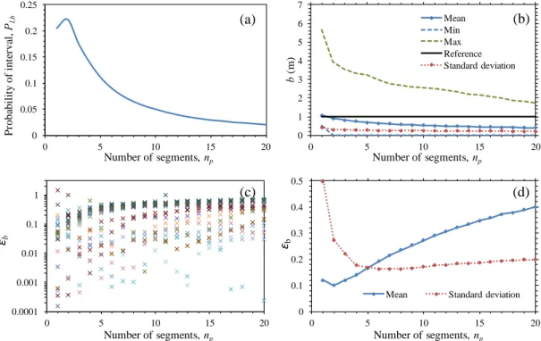
= IDT) to 20 (72, 36, 18, 12, 9, 7, 6, 5, 5, 4, 4, 3, 3, 3, 3, 2, 2, 2, 2, and 2). Figure 3a presents the evolution of the quality estimator (𝑃𝐼,𝑏) with np for 10,000 simulated trajectories. The regular spacing
obtained for np=1 is shown to be not optimal whereas the optimum is found for np=2 with 133 sensors
spaced 37.8 cm in the first segment of 50m and 67 sensors with spacing equal to 74.6cm in the second segment. Figure 3 presents other results to improve the understanding of the causes of this trend. Figure 3b plots the evolution with np of the two first statistics (mean and standard deviation) and the minimum
and maximum values obtained for b from a sample of size 10,000. It is observed that the mean value decreases slightly with np and becomes stable with a significant bias in comparison to the reference
theoretical value (1m). This means that identification algorithm underestimates the value of b. Thus, even if the standard deviation decreases with np, 𝑃𝐼,𝑏 is not optimal for high values of np. Note that the
maximum and minimum bounds are not symmetrical to the mean; Figure 4 illustrates the non-symmetrical distribution of b for a fixed sensor distribution. Figure 3c presents the potential relative error
εb that can reach 4.8 (near 500%) for one realization upon 10,000. The results on Figure 3d show the
mean and standard deviation of εb and confirm that the error on the mean governs the level of the quality
estimator 𝑃𝐼,𝑏 where the minimum value of the mean error is obtained for np=2. Figure 3d also indicates
that there is a significant reduction of the standard deviation of the error from np=1 to 2.
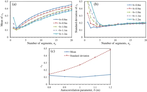
We focus now on the effect of small perturbations around the value of b on the optimal solution. This is a key issue for studying the robustness of the solution obtained from an a priori value of b. This sensitivity analysis studies the effect of b on the error εb by assuming that b takes the following values
around the reference one (i.e., b=1m): 0.8, 0.9, 1, 1.1, and 1.2 m (Figure 5). In the future, more and more data will be available to reduce the uncertainty on the value of b at the design stage as it is already the case for concrete strength for instance, depending on the material parameter of interest, the characteristics of the material, the exposure and on the building process; by focusing on concrete only, large ongoing experimental campaigns are carried out [34] and since only 4 years, more and more researchers are focusing on this challenging issue [5,10,11,23]. That is why we assume a uniform distribution for b with a coefficient of variation of 11%. Figure 5a plots the mean of the error εb for various values of np and b. It is
found that the minimum error corresponds to np = 2 for all values of b. Figure 5b shows that the standard
deviation of the error is sensitive to b for np = 2 and that leads to a given value for np > 5. Figure 5c
presents the mean and standard deviation of the error for np = 2. It is noted that the error on the mean is
almost constant with a minimum for b=1m but the error on the standard deviation increases with b. It is possible to conclude from this trend that under-estimating slightly the value of b reduces the error. This
study illustrate that the methodology is robust even if an error of the future value of b occurs at the design stage. The variability of correlation parameter on a given structure must be estimated by on-going works (see [34] for concrete in sea exposure for example).
4.2. Case of small structures: sensitivity of IDT/L
In the reference case, L and b were respectively of 100 m and 1 m and L>>b. This section analyzes the optimal position of sensors for smaller structures, for fixed b; therefore, we investigate the sensitivity of IDT/L on the quality estimators. For illustration purposes, we keep a large amount of sensors Ns (Ns=200
sensors). Figure 6a and Figure 6b present respectively the effects of six IDT/L ratios on the probability of interval PI,b and the mean of εb. It is shown that the probability of interval PI,b decreases when np increases
and that for large values of IDT/L = 0.2 the probability reaches 0. This result means that the estimation of
b is then not possible whatever np because for IDT/L = 0.2 the length of the structural component is too
short to identify the spatial variability (see Figure 2). Figure 6b confirms this finding where mean of the error εb is larger than 40% for IDT/L =0.2. For different values of IDT/L, it is interesting to note that the
non-regular spacing offers a benefit only when IDT/L remains below 0.03 and that np=2 is optimal in all
these cases. As a conclusion, if the length of the monitored structure is small (L < 40 IDT) the identification error is large and the regular spacing with Lb = IDT should be recommended. On the
contrary for L ≥ 40 IDT, the non-regular spacing with the optimized number of segments np=2 reduces the
identification errors.
4.3. Case of limited number of sensors
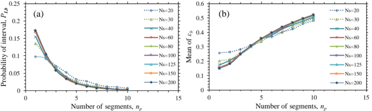
Previous sections considered a large amount of sensors (Ns = 200). However, in real cases, the number of
sensors is limited for technical or economical reasons. We analyze now the effect of limited quantity of sensors by varying their number from 20 to 200. The corresponding results are plotted on Figure 7 and Figure 8, respectively for two cases IDT/L=0.01 (non-regular spacing for long components) and IDT/L=0.04 (regular spacing for short components). It is observed in Figure 7 that the probability of interval PI,b depends on both Ns and np. The interest of implementing a non-regular spacing is significant
only if the number of sensors is large (Ns > 60) where the optimal number of segments is np=2. Moreover
the gain in quality estimator from Ns =80 to 200 is not significant. For a smaller number of sensors (Ns <
60) one segment (np=1) maximizes PI,b: the mean of εb is minimum and is stable on the range 1≤np≤5 for
Ns = 60 and 1≤np≤9 for Ns = 40. On the overall it is noted that a good assessment could obtained for 2 ≤
np ≤6. By deducing an envelope curve from Figure 7, it is possible to plot on Figure 9 an optimal zone of
the couple (Ns, np) that could be used to determine the number of sensors to install.
Figure 8 gives the result for the second case IDT/L=0.04. The results confirm the findings of the previous section for short components where a regular spacing (Lb = IDT) should be recommended.
Moreover, it is also shown that the gain in quality estimator is not significant for Ns varying from 50 to
200.
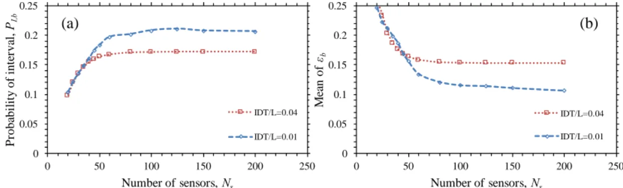
Figure 10 summarizes these results by plotting the optimum values of probability of interval PI,b and
the mean εb with Ns for two ratios: IDT/L=0.01 (non-regular) with np=2 and IDT/L=0.04 (regular) with
np=1. That illustrates more clearly the convergence of results with Ns and that the minimum recommended
value could be Ns=60 sensors.
5. ILLUSTRATION FOR A REAL STUDY CASE
This section applies the proposed methodology and previous findings to two study cases for which real spatially distributed data are available:
• Inspection of the water content along a 16m length reinforced concrete beam placed on the site of IFSTTAR Laboratory, Nantes, France [11]. The measurements were carried out by using a capacitive NDT tool.
• Ultrasonic inspection of the corrosion depth on a corroded 10m length steel sheet-pile of gabion-type wharf in Boulogne, France.
Even if embedded sensors did not perform these measurements, these real data are very helpful to validate the proposed approach.
5.1. Data and modeling
Figure 11 presents the spatial measurements (trajectories) of the water content (RC beam) and corrosion depth (steel sheet-pile). Some values of the corrosion depth trajectory are lacking due mainly to error of
8 measurements and difficulties to measure at specific points during the inspection campaign. For these two trajectories, it is possible to compute the mean and standard deviation for each quantity of interest: • μW = 6.3%, σW = 0.67% for the RC beam (computed from a sample of 80 measurements every 20
cm), and
• μCr = 1.39 mm, σCr = 0.64 mm for the steel sheet-pile (computed from a sample of 1,517
measurements spaced on average every 6.5 mm).
Figure 1 presents the computed autocorrelation values. We obtain a classical shape including negative values [25]. Applying the procedure described in section 3.4 it was found that the exponential correlation functions are appropriate to model the empirical values. The following parameters of the autocorrelation function (eq. 2) were estimated: bW = 0.42m (RC beam) and bCr = 0.11m (steel sheet-pile). These results
are assumed in the following results and discussions as the theoretical values.
Based on the fitted auto-correlation functions, the Inspection Distance Thresholds (IDT) are: IDTW =
0.39m (RC beam) and IDTCr = 0.1m (steel sheet-pile). Taking into account the length of the structural
components and the findings of section 4, it is possible to propose two types of sensors spacing:
• a regular spacing of measurements for the RC beam because the ratio IDTW/L=0.39/16=0.025≥1/40; and
• a non-regular spacing for the steel sheet-pile because the ratio IDTCr/L = 0.1/12 < 1/40.
The following section compares real and numerical estimations to determine the appropriateness of the proposed sensor spacing in each case.
5.2. Comparison with real databases
This section estimates the errors on the identification of εb for both real data and simulations for the two
study cases. Numerical simulations are based on: (i) the procedures described in section 2 to generate trajectories, and (ii) the values of mean, standard deviation and autocorrelation parameter identified in section 5.1. The main goal of this section is to validate the proposed numerical approach as well as to verify if the practical recommendations of the numerical findings of section 5.1 could be applied to real measures.
Figure 12a compares the evolution of the error of the assessment of b by considering various np for
results obtained from simulations and those computed from real data measured on the RC beam. The numerical mean as well as the minimum and maximum values were computed from 10,000 simulations. The results show that the numerical and mean values are close and that εb is minimum for np = 1. This
behavior confirms the recommendation based on the numerical findings for the case of L < 40IDT where the regular spacing is suggested in such a case. Figure 12b compares the evolution of the mean of εb with
Ns for np=1 and np=2. It is observed that the mean of εb decreases when more information from additional
sensors is considered. There is a convergence in the error that is faster when np=1; in such a case it is
reached for Ns > 30 sensors. The results also show that a regular spacing with np=1 leads to lower error
for both simulated and real data.
Figure 13 plots similar results to those presented in Figure 12 for the steel sheet-pile. Figure 13a confirms that the non-regular spacing is appropriated to reduce εb in this case where L ≥ 40IDT. Figure
13b shows the effect of the numbers of sensors Ns on the mean of εb. Results on Figure 13 indicate that
the error is lower for np=2. They also show that there is a convergence trend for the mean of εb when the
number of sensor increases; in this case it can be concluded that Ns=45 sensors are sufficient to satisfy the
quality requirement.
6. CONCLUSIONS
SHM of new structures is increasing and offers an opportunity for using embedded sensors for uncertainty and spatial variability quantification. Information provided by SHM will be also very useful to plan destructive and NDT measurements for assessing supplementary data required for improving lifetime assessment and optimizing maintenance actions. This paper proposed an original method for defining a non-regular spacing of sensors devoted to the assessment of the autocorrelation function parameter of stationary fields. The method is based on the probabilistic identification of the autocorrelation function parameter and aims at reducing the error on its estimation. Numerical simulations of Gaussian stationary stochastic fields illustrate the potential of the method by providing a decision aid tool when a limited number of sensors is available. Based on these numerical results, it was found that the position of sensors is a key factor for estimating the autocorrelation function parameter. This methodology requires an a priori knowledge of the ACF which might be difficult to obtain before installing the sensors even if
several experimental studies focus on spatial variability characterization; therefore, a sensitivity study showed that the methodology was robust with a tolerance on the exact value.
The main results allow to propose a criterion for regular or non regular spacing of sensors along the inspection zone depending on the component length and autocorrelation structure of the random field: (i) regular spacing is recommended for the case L < 40IDT, and (ii) non-regular spacing is suggested for the case L ≥ 40IDT. The paper shows also the important role of the position of sensors in the estimation of the autocorrelation function parameter. Even if only two segments are shown to be sufficient in the 1D case, it helps to decrease the number and therefore the cost of sensors and data treatment and this gain will increase in the 2D case.
7. AKNOWLEDGEMENTS
The authors would like to acknowledge the Pays de la Loire Region for supporting the projects ECND-PdL and SI3M as well as the European commission for funding the DuratiNet EC Interreg project (http://www.duratinet.org).
8. REFERENCES
[1] Stewart MG. Spatial variability of pitting corrosion and its influence on structural fragility and reliability of RC beams in
flexure. Structural Safety 2004;26:453–70.
[2] Li J, Masia MJ, Stewart MG, Lawrence SJ. Spatial variability and stochastic strength prediction of unreinforced masonry
walls in vertical bending. Engineering Structures 2014;59:787–97. doi:10.1016/j.engstruct.2013.11.031.
[3] Li Y. Effect of spatial variability on maintenance and repair decisions for concrete structures. Delft University, Delft,
Netherlands, 2004.
[4] Srivastava A. Spatial Variability Modelling of Geotechnical Parameters and Stability of Highly Weathered Rock Slope.
Indian Geotechnical Journal 2012;42:179–85.
[5] O’Connor A, Kenshel O. Experimental Evaluation of the Scale of Fluctuation for Spatial Variability Modeling of
Chloride-Induced Reinforced Concrete Corrosion. Journal Of Bridge Engineering 2013;18:3–14.
[6] Griffiths DV, Fenton GA. Influence of soil strength spatial variability on the stability of an undrained clay slope by finite
elements. Slope Stability 2000 ASCE 2000:184–93.
[7] Pasqualini O, Schoefs F, Chevreuil M, Cazuguel M. Measurements and statistical analysis of fillet weld geometrical
parameters for probabilistic modelling of the fatigue capacity. Marine Structures 2013;34:226–48.
doi:10.1016/j.marstruc.2013.10.002.
[8] Nguyen NT, Sbartaï Z-M, Lataste J-F, Breysse D, Bos F. Assessing the spatial variability of concrete structures using
NDT techniques – Laboratory tests and case study. Construction and Building Materials 2013;49:240–50. doi:10.1016/j.conbuildmat.2013.08.011.
[9] Nguyen NT, Sbartaï ZM, Lataste J-F, Breysse D, Bos F. Non-destructive evaluation of the spatial variability of reinforced
concrete structures. Mechanics & Industry 2014;16:103. doi:10.1051/meca/2014064.
[10] Gomez-Cardenas C, Sbartaï ZM, Balayssac JP, Garnier V, Breysse D. New optimization algorithm for optimal spatial
sampling during non-destructive testing of concrete structures. Engineering Structures 2015;88:92–9.
doi:10.1016/j.engstruct.2015.01.014.
[11] Schoefs F, Bastidas-Arteaga E, Tran TV, Villain G, Derobert X. Characterization of random fields from NDT
measurements: A two stages procedure. Engineering Structures 2016;111:312–22. doi:10.1016/j.engstruct.2015.11.041.
[12] Hu W-H, Thöns S, Rohrmann RG, Said S, Rücker W. Vibration-based structural health monitoring of a wind turbine
system. Part I: Resonance phenomenon. Engineering Structures 2015;89:260–72. doi:10.1016/j.engstruct.2014.12.034.
[13] Ye XW, Ni YQ, Wong KY, Ko JM. Statistical analysis of stress spectra for fatigue life assessment of steel bridges with
structural health monitoring data. Engineering Structures 2012;45:166–76. doi:10.1016/j.engstruct.2012.06.016.
[14] Kulprapha N, Warnitchai P. Structural health monitoring of continuous prestressed concrete bridges using ambient
thermal responses. Engineering Structures 2012;40:20–38. doi:10.1016/j.engstruct.2012.02.001.
[15] Schoefs F, Clement A, Nouy A. Assessment of spatially dependent ROC curves for inspection of random fields of defects.
Structural Safety 2009;31:409–19.
[16] Sheils E, O’Connor A, Schoefs F, Breysse D. Investigation of the effect of the quality of inspection techniques on the
optimal inspection interval for structures. Structure and Infrastructure Engineering 2012;8:557–68.
doi:10.1080/15732479.2010.505377.
[17] Bastidas-Arteaga E, Schoefs F. Stochastic improvement of inspection and maintenance of corroding reinforced concrete
structures placed in unsaturated environments. Engineering Structures 2012;41:50–62.
doi:10.1016/j.engstruct.2012.03.011.
[18] Bastidas-Arteaga E, Schoefs F. Sustainable maintenance and repair of RC coastal structures. Proceedings of the Institution
of Civil Engineers - Maritime Engineering 2015;168:162–73. doi:10.1680/jmaen.14.00018.
[19] Schöberl M, Keinert J, Ziegler M, Seiler J, Niehaus M, Schuller G, et al. Evaluation of a high dynamic range video
10
[20] Bazant Z, Xi Y. Statistical Size Effect in Quasi-brittle Structures: II. Nonlocal Theory. ASCE J of Engrg Mech
1991;117:2623–40.
[21] Bazant Z, Novák D. Probabilistic Nonlocal Theory for Quasibrittle Fracture Initiation and Size Effect. I: Theory. Journal
of Engineering Mechanics 2000;126:166–74.
[22] Bazant Z, Novák D. Probabilistic Nonlocal Theory for Quasibrittle Fracture Initiation and Size Effect. II: Application.
Journal of Engineering Mechanics 2000;126:175–85.
[23] Stewart MG. Spatial Variability of Damage and Expected Maintenance Costs for Deteriorating RC Structures. Structure
and Infrastructure Engineering 2006;2:79–96.
[24] Nobahar A. Effects of soil spatial variability on soil-structure interaction. PhD Thesis, Memorial University, St. John’s,
NL., 2003.
[25] Chenari RJ, Dodaran RO. New method for estimation of the scale of fluctuation of geotechnical properties in natural
deposits. Computational Methods in Civil Engineering 2010;1:55–66.
[26] Jaksa MB. Experimental evaluation of the scale of fluctuation of a stiff clay. In: Melchers RE, Stewart MG, editors. Proc.
8th Int. Conf. on the Application of Statistics and Probability, Sydney: Balkema; 1999, p. 415–22.
[27] Pasqualini O, Schoefs F, Chevreuil M, Cazuguel M. Statistical analysis of welded joints geometry for stochastic modeling
and reliability analysis. In: ASRANeT, editor. 6th Conference on Network for Integrating Structural Analysis, Risk and Reliability (ASRANet), London (UK): 2012.
[28] Ray A. Stochastic Measure of Fatigue Crack Damage for Health Monitoring of Ductile Alloy Structures. Structural Health
Monitoring 2004;3:245–63. doi:10.1177/1475921704045626.
[29] Li C-C, Der Kiureghian A. Optimal Discretization of Random Fields. Journal of Engineering Mechanics 1993;119:1136–
54. doi:10.1061/(ASCE)0733-9399(1993)119:6(1136).
[30] Ghanem RG, Spanos PD. Stochastic Finite Elements: A Spectral Approach. New York, USA: Springer; 1991.
[31] Vanmarcke E. Random fields: analysis and synthesis. Mass, London: MIT Press, Cambridge; 1983.
[32] Ravahatra NR, Duprat F, Schoefs F, de Larrard T, Bastidas-Arteaga E, Rakotovao Ravahatra N, et al. Assessing the
capability of analytical carbonation models to propagate uncertainties and spatial variability of reinforced concrete structures. Frontiers in Built Environment 2017;3:1. doi:10.3389/FBUIL.2017.00001.
[33] Kenshel O. Influence of spatial variability on whole life management of reinforced concrete bridges. University of Dublin,
Trinity College, Dublin, Ireland, 2009.
[34] Boureau L, Bouteiller V, Schoefs F, Gaillet L, Thauvin B, Schneider J, et al. On-site corrosion monitoring – reliability.
International RILEM Conference on Materials, Systems and Structures in Civil Engineering - Conference segment on Electrochemistry in Civil Engineering, DTU, Lyngby, Denmark: 2016.
Figure 1. Auto-correlation data and fitted ACFs for water content in a RC beam (IFSTTAR, Nantes, France) and corrosion in a steel sheet-pile (Boulogne, France).
Figure 2. Representation of high correlation zones and non-regularly spacing sensors (Ns=23 sensors
and np=3 segments) along a trajectory of the random field Z(x, θ) and estimated autocorrelation. -0.4 -0.2 0 0.2 0.4 0.6 0.8 1 0 4 8 12 16 A u to -c o rr el at io n ( ρ) Distance (m) Measure Approximation -0.6 -0.4 -0.2 0 0.2 0.4 0.6 0.8 1 0 0.5 1 1.5 2 2.5 A u to -c o rr el at io n ( ρ) Distance (m) Measure Approximation
Water content Corrosion depth
Measure Model eq. (2)
§§
Measure Model eq. (2) 0 1 2 3 4 5 6 7 8 9 10 11 12 13 14 15 16R
an
d
o
m
f
ie
ld
,
Z
(x
,q
)
Distance (m)
-0.4 -0.2 0 0.2 0.4 0.6 0.8 1 0 1 2 3 4 5 6 7 8 9 10 11 12 13 14 15 16A
u
to
-c
o
rr
el
at
io
n
(
r)
Distance (m)
Sensors Fitted ACF Sensors Random field Lm=L/3 L Lm=L/3 Lm=L/3 Nc3=3 Nc2=7 Nc1=13 Lb1 Lb2 Lb312 Figure 3. Effect of number of segments np on: (a) the probability of interval PI,b, (b) the estimated
values of the auto-correlation parameter b (c) the distribution of εb, and (d) the mean and standard
deviation of εb (Ns=200, L=100m and =10%).
Figure 4. Distribution of estimated auto-correlation parameter 𝑏̂ for Ns=200 and np=2.
0 0.05 0.1 0.15 0.2 0.25 0 5 10 15 20 P ro b ab il it y o f in te rv al , PI,b Number of segments, np 0 0.1 0.2 0.3 0.4 0.5 0 5 10 15 20 εb Number of segments, np
Mean Standard deviation 0 1 2 3 4 5 6 7 0 5 10 15 20 b (m ) Number of segments, np Mean Min Max Reference Standard deviation (a) (b) 0.0001 0.001 0.01 0.1 1 0 5 10 15 20 εb Number of segments, np (c) (d)
Figure 5. Sensitivity of εb for: (a) the mean of εb, (b) the standard deviation of εb, and (c) the mean and
standard deviation of εb for np=2 (Ns=200, L=100m).
Figure 6. Effect of ratio IDT/L on (a) the probability of interval PI,b, and (b) the mean of εb as a
function of the number of segments np (Ns=200 and =10%).
0 0.1 0.2 0.3 0.4 0.5 0 5 10 15 20 M ea n o f εb Number of segments, np b=0.8m b=0.9m b=1.0m b=1.1m b=1.2m 0 0.1 0.2 0.3 0.4 0.5 0 5 10 15 20 S ta n d ar d d ev ia ti o n o f εb Number of segments, np b=0.8m b=0.9m b=1.0m b=1.1m b=1.2m 0 0.1 0.2 0.3 0.4 0.5 0.8 0.9 1 1.1 1.2 εb Autocorrelation parameter, b (m) Mean Standard deviation (c) (a) (b) 0 0.05 0.1 0.15 0.2 0.25 0 5 10 15 20 P ro b ab il it y o f in te rv al P I, b Number of segments, np IDT/L=0,2 IDT/L=0,05 IDT/L=0,04 IDT/L=0,025 IDT/L=0,02 IDT/L=0,01 0 0.2 0.4 0.6 0.8 1 0 5 10 15 20 M ea n o f εb Number of segments, np (a) (b)
14 Figure 7. Effect of Ns on (a) the probability of interval PI,b, and (b) the mean of εb, for various Ns
(IDT/L=0.01 and =10%).
Figure 8. Effect of Ns on (a) the probability of interval PI,b, and (b) the mean of εb, for various Ns
(IDT/L=0.04 and =10%).
Figure 9. Definition of optimal zone for determining the number of sensors as a function of the number of segments (IDT/L=0.01 and =10%).
0 0.05 0.1 0.15 0.2 0.25 0.3 0 5 10 15 P ro b ab il it y o f in te rv al , PI,b Number of segments, np Ns=20 Ns=30 Ns=40 Ns=60 Ns=80 Ns=100 Ns=125 Ns=150 Ns=200 0 0.05 0.1 0.15 0.2 0.25 0.3 0.35 0 5 10 15 M ea n o f εb Number of segments, np Ns=20 Ns=30 Ns=40 Ns=60 Ns=80 Ns=100 Ns=125 Ns=150 Ns=200 (a) (b) 0 0.05 0.1 0.15 0.2 0.25 0 5 10 15 P ro b ab il it y o f in te rv al , PI,b Number of segments, np Ns=20 Ns=30 Ns=40 Ns=60 Ns=80 Ns=100 Ns=125 Ns=150 Ns=200 0 0.1 0.2 0.3 0.4 0.5 0.6 0 5 10 15 M ea n o f εb Number of segments, np Ns=20 Ns=30 Ns=40 Ns=60 Ns=80 Ns=100 Ns=125 Ns=150 Ns=200 (a) (b)
0
2
4
6
8
10
12
0
50
100
150
200
250
N
u
m
b
er
o
f
se
g
m
en
ts
,
n
pNumber of sensors, N
sOptimal zone
Figure 10. Effect of Ns on (a) the probability of interval PI,b, and (b) the mean of εb, for =10% and np
optimized.
Figure 11. Experimental trajectories of water content (up) and corrosion (down).
0 0.05 0.1 0.15 0.2 0.25 0 50 100 150 200 250 P ro b ab il it y o f in te rv al , PI,b Number of sensors, Ns IDT/L=0.04 IDT/L=0.01 0 0.05 0.1 0.15 0.2 0.25 0 50 100 150 200 250 M ea n o f εb Number of sensors, Ns IDT/L=0.04 IDT/L=0.01 (a) (b) 0 2 4 6 8 10 0 1 2 3 4 5 6 7 8 9 10
C
o
rr
o
si
o
n
d
ep
th
(
m
m
Distance (m)
3 4 5 6 7 8 9 0 2 4 6 8 10 12 14 16W
at
er
c
o
n
te
n
t
(%
)
Distance (m)
Measures on a RC beam at IFSTTAR, Nantes-France
Measures on a steel sheet-pile at Boulogne-France
0 2 4 6
16 Figure 12. Comparison between simulated results and real inspection values in the case of water content
(RC beam, L =16 m, IDT=0.4m): (a) effect of np on εb, for Ns=40 sensors (b) effect of Ns on the mean
of εb.
Figure 13. Comparison between simulated results and real inspection values in the case of corrosion depth (steel sheet-pile, L =12 m, IDT=0.1m): (a) effect of np on εb, for Ns=40 sensors (b) effect of Ns on the
mean of εb. 0 0.1 0.2 0.3 0.4 0.5 0 1 2 3 4 5 6 εb Number of segments, np Min Mean Max Real Numerical result (a) 0.1 0.2 0.3 0.4 0.5 0 20 40 60 80 100 M ea n o f εb Number of sensors, Ns np=1 Real np=2 Real Numerical: np=1 Real: np=1 Numerical: np=2 Real: np=2 (b) (a) (b) 0 0.1 0.2 0.3 0.4 0.5 0 1 2 3 4 5 6 εb Number of segments, np Min Mean Max Real 0.1 0.2 0.3 0.4 0.5 0 20 40 60 80 100 120 M ea n o f εb Number of sensors, Ns np=1 Real np=2 Real Numerical: np=1 Real: np=1 Numerical: np=2 Real: np=2 Numerical result