Smart motion sensor for navigated prosthetic surgery

HAL Id: pastel-00691192

https://pastel.archives-ouvertes.fr/pastel-00691192

Submitted on 25 Apr 2012

HAL is a multi-disciplinary open access archive for the deposit and dissemination of sci-entific research documents, whether they are pub-lished or not. The documents may come from

L’archive ouverte pluridisciplinaire HAL, est destinée au dépôt et à la diffusion de documents scientifiques de niveau recherche, publiés ou non, émanant des établissements d’enseignement et de

Göntje Caroline Claasen

To cite this version:

Göntje Caroline Claasen. Smart motion sensor for navigated prosthetic surgery. Other. Ecole Na-tionale Supérieure des Mines de Paris, 2012. English. �NNT : 2012ENMP0008�. �pastel-00691192�

T

H

È

S

Doctorat ParisTech

T H È S E

pour obtenir le grade de docteur délivré par

l’École Nationale Supérieure des Mines de Paris

Spécialité “Mathématique et Automatique”

présentée et soutenue publiquement par

Göntje Caroline CLAASEN

le 17 février 2012

Capteur de mouvement intelligent

pour la chirurgie prothétique naviguée

Directeur de thèse:Philippe MARTIN

Jury

Mme Isabelle FANTONI-COICHOT, Chargée de recherche HDR, Rapporteur Heudiasyc UMR CNRS 6599, Université de Technologie de Compiègne

M. Philippe POIGNET, Professeur, LIRMM UM2-CNRS Rapporteur

M. Tarek HAMEL, Professeur, I3S UNSA-CNRS Examinateur

M. Wilfrid PERRUQUETTI, Professeur, LAGIS FRE CNRS 3303-UL1-ECL Examinateur

M. Frédéric PICARD, Docteur en médecine, chirurgien orthopédiste, Examinateur

Golden Jubilee National Hospital, Glasgow

T

H

È

S

ParisTech

P H D T H E S I S

To obtain the Doctor’s degree from

École Nationale Supérieure des Mines de Paris

Speciality “Mathématique et Automatique”

defended in public by

Göntje Caroline CLAASEN

on February 17, 2012

Smart motion sensor

for navigated prosthetic surgery

Committee

Ms. Isabelle FANTONI-COICHOT,Chargée de recherche HDR, Reviewer Heudiasyc UMR CNRS 6599, Université de Technologie de Compiègne

Mr. Philippe POIGNET, Professor, LIRMM UM2-CNRS Reviewer

Mr. Tarek HAMEL, Professor, I3S UNSA-CNRS Examiner

Mr. Wilfrid PERRUQUETTI, Professor, LAGIS FRE CNRS 3303-UL1-ECL Examiner

Mr. Frédéric PICARD, MD, Orthpaedic Surgeon, Golden Jubilee National Hospital, Glasgow Examiner

Centre Automatique et Systèmes Unité Mathématiques et Systèmes MINES ParisTech

60 boulevard St Michel 75272 Paris Cedex France.

E-mail: caroline.claasen@mines-paristech.fr, goentje.claasen@gmx.de

Key words. - optical-inertial data fusion, Kalman filtering, nonlinear observers, computer-assisted surgery, servo-controlled handheld tool

Mots clés. - fusion de données optiques-inertielles, filtrage de Kalman, observateurs non-linéaires, chirurgie assistée par ordinateur, outil à main asservi

Tout d’abord je tiens à remercier Philippe Martin pour avoir encadré cette thèse pendant trois ans. Merci de votre enthousiasme pour ce projet, pour la recherche en générale et pour les choses qui marchent. Merci pour votre soutien et vos conseils.

Je souhaite remercier Isabelle Fantoni-Coichot ainsi que Philippe Poignet qui ont accepté d’être les rapporteurs de cette thèse. Je remercie également Tarek Hamel, Wilfrid Perruquetti et Frédéric Picard qui m’ont fait l’honneur de participer au jury de soutenance. Un grand merci à tous les membres du Centre Automatique et Systèmes pour leur soutien et leurs conseils et pour avoir répondu à mes nombreuses questions sur la France et la langue française. Merci à mes camarades de thèse Eric, Florent et Pierre-Jean. Merci également à Erwan pour son aide.

I would like to thank Frédéric Picard and Angela Deakin from the Golden Jubilee Hospital in Glasgow for having introduced me to the world of orthopaedic surgery.

Danke meiner Familie, besonders meinen Eltern und Großeltern, der Familie Bezanson und natürlich Gregor für ihre immerwährende Unterstützung, die dieses Abenteuer erst möglich gemacht hat.

Smart motion sensor

Nous présentons un système de tracking optique-inertiel qui consiste en deux caméras stationnaires et une Sensor Unit avec des marqueurs optiques et une centrale inertielle. La Sensor Unit est fixée sur l’objet suivi et sa position et son orientation sont déterminées par un algorithme de fusion de données. Le système de tracking est destiné à asservir un outil à main dans un système de chirurgie naviguée ou assistée par ordinateur. L’algorithme de fusion de données intègre les données des différents capteurs, c’est-à-dire les données optiques des caméras et les données inertielles des accéléromètres et gyroscopes. Nous présentons différents algorithmes qui rendent possible un tracking à grande bande passante avec au moins 200Hz avec des temps de latence bas grâce à une approche directe et des filtres dits invariants qui prennent en compte les symétries du système. Grâce à ces propriétés, le système de tracking satisfait les conditions pour l’application désirée. Le système a été implémenté et testé avec succès avec un dispositif expérimental.

Abstract

We present an optical-inertial tracking system which consists of two stationary cameras and a Sensor Unit with optical markers and an inertial measurement unit (IMU). This Sensor Unit is attached to the object being tracked and its position and orientation are determined by a data fusion algorithm. The tracking system is to be used for servo-controlling a handheld tool in a navigated or computer-assisted surgery system. The data fusion algorithm integrates data from the different sensors, that is optical data from the cameras and inertial data from accelerometers and gyroscopes. We present different algorithms which ensure high-bandwidth tracking with at least 200Hz with low latencies by using a direct approach and so-called invariant filters which take into account system symmetries. Through these features, the tracking system meets the requirements for being used in the desired application. The system was successfully implemented and tested with an experimental setup.

Contents

1 Introduction 1

1.1 Navigated Surgery Systems . . . 2

1.2 Handheld Tools for Navigated Surgery . . . 5

1.3 Smart Handheld Tool . . . 6

1.4 Tracking for the Smart Handheld Tool . . . 7

1.5 Servo-Control for 1D model . . . 9

1.6 Outline . . . 14

1.7 Publications . . . 15

2 Optical-Inertial Tracking System 17 2.1 System Setup . . . 17 2.1.1 Optical System . . . 17 2.1.2 Inertial Sensors . . . 22 2.2 Mathematical Model . . . 24 2.2.1 Coordinate systems . . . 24 2.2.2 Quaternions . . . 24 2.2.3 Dynamics Model . . . 27 2.2.4 Output Model . . . 27 2.2.5 Noise Models . . . 28 2.2.6 Complete Model . . . 31

3 State of the Art 33 3.1 Computer Vision and Optical Tracking . . . 33

3.1.1 Monocular Tracking . . . 34

3.1.2 Stereo Tracking . . . 37

3.1.3 Problems/Disadvantages . . . 50

3.2 Optical-Inertial Tracking Systems . . . 50

3.2.1 Systems Presented in the Literature . . . 50

3.2.2 Motivation of Our Approach . . . 53

3.3.1 Camera Calibration . . . 54

3.3.2 IMU Calibration . . . 55

3.3.3 Optical-Inertial Calibration . . . 57

4 Data Fusion 59 4.1 Motivation . . . 59

4.2 Extended Kalman Filter . . . 61

4.2.1 Continuous EKF . . . 61

4.2.2 Multiplicative EKF (MEKF) . . . 62

4.2.3 Continuous-Discrete EKF . . . 63

4.3 Data Fusion for Optical-Inertial Tracking . . . 64

4.3.1 System Observability . . . 64

4.3.2 Direct and Indirect Approaches . . . 65

4.3.3 MEKF . . . 65

4.3.4 Right- and Left-Invariant EKF . . . 67

4.3.5 Covariance Parameters . . . 77

4.3.6 Continuous-Discrete and Multi-rate . . . 77

4.4 RIEKF for Calibration . . . 79

4.4.1 Influence of calibration errors on the RIEKF . . . 80

4.4.2 Calibration of Marker-Body Rotation with RIEKF . . . 87

5 Implementation and Experimental Results 89 5.1 Experimental Setup . . . 89

5.1.1 Cameras and Optical Markers . . . 89

5.1.2 Inertial Sensors . . . 94 5.1.3 Sensor Unit . . . 94 5.1.4 Data Acquisition . . . 94 5.1.5 Algorithm Implementation . . . 97 5.1.6 Tracking References . . . 103 5.2 Experiments . . . 106

5.2.1 Experiment 1: static case . . . 106

5.2.2 Experiment 2: slow linear motion . . . 106

5.2.3 Experiment 3: fast oscillating linear motion . . . 106

5.2.4 Experiment 4: static orientations . . . 106

5.3 Results . . . 110

5.3.1 General Observations . . . 110

5.3.2 Precision and Accuracy . . . 118

5.3.3 High-Bandwidth Tracking . . . 119

5.3.4 Influence of Sensor Unit Calibration . . . 124

5.4.1 Optical System . . . 128

5.4.2 Accelerometers . . . 129

5.4.3 Gyroscopes . . . 130

5.4.4 Sensor Unit . . . 130

Chapter 1

Introduction

Les systèmes de chirurgie assistée par ordinateur sont de plus en plus utilisés dans les salles opératoires. Pour la pose de prothèses de genou, par exemple, un tel système mesure des points anatomiques, calcule la position optimale de la prothèse et indique les lignes de coupe. Actuellement, les coupes sont exécutées à l’aide de guides de coupe mécaniques, mais une technique de coupe sans guide mécanique est demandée par les chirurgiens. Différentes méthodes ont été proposées, par exemple utilisant un feedback visuel pour le chirurgien ou des systèmes robotiques. Nous considérons un outil à main asservi qui utilise un système de tracking pour déterminer la position de l’outil par rapport au patient et aux plans de coupe désirés. Le tracking doit avoir une bande passante d’au moins 200Hz pour pouvoir suivre le mouvement rapide de l’outil.

Comme aucun système adapté aux conditions de la salle opératoire et au coût possible d’un système de chirurgie n’existe, nous proposons un nouveau système de tracking qui utilise des capteurs optiques et inertiels pour déterminer la position et l’orientation d’un outil à main asservi.

Le système a une grande bande passante grâce aux capteurs inertiels haute fréquence. Il a un temps de latence réduit par rapport à des systèmes similaires grâce à deux caractéristiques: nous proposons une approche directe utilisant les données brutes des capteurs sans faire des calculs complexes comme dans l’approche standard, et nous utilisons des algorithmes de fusion de données qui prennent en compte les symmétries du système ce qui réduit le temps de calcul.

Nous présentons des résultats de simulation pour un modèle simple d’un outil à main asservi avec différents systèmes de tracking illustrant l’intérêt d’un tel systéme.

1.1

Navigated Surgery Systems

Computer-assisted or navigated surgery systems have become more and more common in operating rooms over the last 15 years [DiGioia et al., 2004].

In orthopedic surgery systems, e.g. for knee replacement, it is important to make accurate bone cuts and place the prosthesis correctly. The system acquires relevant patient anatomical landmarks and calculates appropriate prosthesis placement based on built up frame of reference. It then defines the desired cutting planes for the knee prosthesis [DiGioia et al., 2004]. Such a computer-assisted surgery system for knee replacement is described in detail in [Stulberg et al., 2004].

Here we consider so-called image-free or CT-free surgery systems. Image-guided systems [Jolesz et al., 1996] use image data from video, computer tomography (CT), magnetic-resonance imaging (MRI) or ultrasound (US) to obtain patient anatomical information before and during surgery. These imaging techniques demand for important processing and some, like CT scans, also expose the patient to radiation. In contrast to this, image-free systems use optical tracking to determine anatomical landmarks [Mösges and Lavallé, 1996, DiGioia et al., 2004]. They make use of cameras but unlike image-based systems they do not treat the whole image. Instead, the cameras observe optical markers which are attached to the patient’s bones. The optical markers are detected in the images and only the information of their point coordinates are used in the subsequent analysis instead of the whole image. The first image-free system for knee replacement used in an operating room was presented in [Leitner et al., 1997]. This system was later commercialized as OrthoPilot (Aesculap AG, Tuttlingen, Germany [Aesculap AG, 2011]). Figure 1.1 shows the OrthoPilot.

It is important to note the difference between computer-assisted surgery systems and robotic surgery systems. In the latter, surgical procedures are executed autonomously by a robotic system [Taylor and Stoianovici, 2003]. Robotic systems can perform these procedures with high accuracy but rise questions about safety and liability [Davies, 1996]. Computer-assisted surgery systems on the other hand, let the surgeon keep the control over the whole surgical procedure.

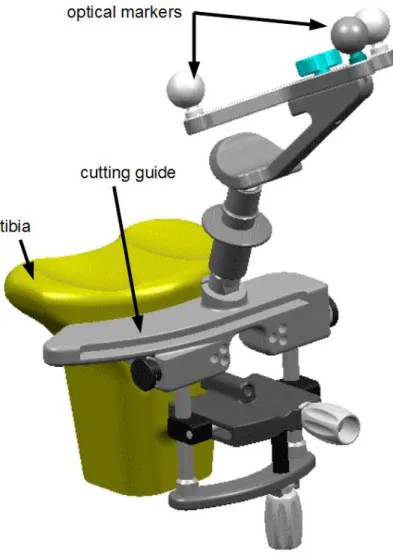
We now return to the original problem of cutting bones for knee replacement. In current systems, the bone cuts are executed with the help of cutting guides (also called cutting jigs) which are fixed to the patient’s bone in accordance with the desired cutting planes [Stulberg et al., 2004]. They guide the bone saw mechanically with good accuracy. A cutting guide is depicted in Figure 1.2. Cutting guides have two main drawbacks: Mounting and repositioning the guide takes time and the procedure is invasive because the guide is pinned to the bone with screws.

Figure 1.1: OrthoPilot® orthopaedic navigation system for knee replacement. Copyright Aesculap AG

1.2

Handheld Tools for Navigated Surgery

Using a handheld saw without any cutting guides would have several advantages: the procedure would be less invasive, demand less surgical material and save time. Obviously, it would have to produce cuts with the same or even better accuracy to be a valuable improvement.

While a robotic system could achieve this task of cutting along a desired path, many surgeons wish to keep control over the cutting procedure. Therefore, an intelligent handheld tool should be used which combines the surgeon’s skills with the accuracy, precision and speed of a computer-controlled system. Such a tool should be small and lightweight so as not to impede on the surgeon’s work, compatible with existing computer-assisted surgery systems and relatively low-cost.

Controlling the tool position and keeping it along the desired cutting path necessitate the following steps:

1. define desired cutting plane relative to the patient,

2. track tool position and orientation relative to the patient and

3. compare desired and actual positions and correct the tool position accordingly. The first step is done by the surgery system and the second by a tracking system. Step 3 can be executed either by the surgeon, by a robotic arm or directly by the handheld tool. Several handheld tools have been developed in recent years, employing different strategies for the control of the tool position. In [Haider et al., 2007], the patient’s bone and a handheld saw are tracked by an optical tracking system and the actual and desired cutting planes are shown on a screen. The surgeon corrects the position of the saw based on what he sees on the screen to make the actual and desired planes coincide. This approach is called "navigated freehand cutting" by the authors. A robotic arm is used in [Knappe et al., 2003] to maintain the tool orientation and correct deviations caused by slipping or inhomogeneous bone structure. The arm is tracked by an optical tracking system and internal encoders. The optical tracking also follows the patient’s position. In [Maillet et al., 2005], a cutting guide is held by a robotic arm at the desired position, thus eliminating the problems linked to attaching cutting guides to the bone and repositioning. Several commercial systems with robotic arms are available, for example the Mako Rio (Mako Surgical, Fort Lauderdale, USA [Mako Surgical Corp., 2011]) and the Acrobot Sculptor (Acrobot LTD) [Jakopec et al., 2003].

Several "intelligent" handheld tools which are able to correct deviations from the desired cutting plane automatically by adapting the blade/drill position without a robotic arm have been developed. The systems presented in [Brisson et al., 2004] and [Kane et al., 2009] use an optical tracking system. [Schwarz et al., 2009] uses an

optical tracking system to determine the position of the patient and of the tool which also contains inertial sensors. The authors estimated the necessary tracking frequency to be of 100Hz to be able to compensate the surgeon’s hand tremor which range is up to 12 Hz and the patient’s respiratory motion.

The systems presented so far determine a desired cutting path based on absolute position measurements of tools and patients. In contrast, tools have been developed which are controlled relative to the patient only. [Ang et al., 2004] presents a handheld tool which uses accelerometers and magnetometers for tremor compensation. A handheld tool with actuators controlling the blade position is presented in [Follmann et al., 2010]. The goal is to cut the skull only up to a certain depth while the surgeon guides the tool along a path. While an optical tracking system is used in this work, an alternative version with a tracking system using optical and inertial sensors is presented in [Korff et al., 2010]. Three different approaches to bone cutting without cutting guides have been compared in [Cartiaux et al., 2010]: freehand, navigated freehand (surgeon gets visual feedback provided by a navigation system; similar to [Haider et al., 2007]) and with an industrial robot. The authors find that the industrial robot gives the best result and freehand cutting the worst.

The authors of [Haider et al., 2007] compared their navigated freehand cuts to those with conventional cutting jigs and found the cuts had rougher surfaces but better alignment.

1.3

Smart Handheld Tool

The handheld tool we consider here is supposed to be an extension for an image-free or image-based computer-assisted surgery system, hence it can make use of an optical tracking system but not of an active robotic arm. The tool is to be servo-controlled with motors in the tool joints which can change the blade position. We use a saw as an example but the same applies to drilling, pinning or burring tools. In the case of a saw for knee replacement surgery, the new smart handheld tool would eliminate the need for cutting guides.

The tracking system and particularly its bandwidth are a key for good performance of the servo-control. Firstly, the tracking system should be able to follow human motion and especially fast movements - these could be due to a sudden change of bone structure while cutting or to slipping of the surgeon’s hand. These are the movements to be corrected. Secondly, it should be fast enough to let the servo-control make the necessary corrections. The faster the correction, the smaller the deviation will be. Finally, the servo-control should make the correction before the surgeon notices the error to avoid conflict between the control and the surgeon’s reaction. We estimate the surgeon’s perception time to be

of 10ms which corresponds to a frequency of 100Hz and therefore consider the necessary bandwidth for the tracking system to be at least 200Hz.

Commercially available optical tracking systems suitable for surgery have a bandwidth of only 60Hz, thus ruling out the use of this type of tracking for the smart handheld tool. Alternatively, there are are electro-magnetic, mechanical and inertial tracking technologies. Electro-magnetic sensors are difficult to use in an operating room because of interferences of the electro-magnetic field with the surgical material. A robotic arm would provide mechanical tracking of the handheld tool but has been excluded because it would be too constrictive for the surgeon. Inertial sensors cannot be used on their own because of their drifts which cannot be compensated.

We propose to use a novel tracking system using both inertial and optical sensors which will be described in the next Section.

1.4

Tracking for the Smart Handheld Tool

In this thesis, we propose an optical-inertial tracking system which combines an optical tracking system with inertial sensors. These inertial sensors have a high bandwidth of typically 100-1000Hz [Groves, 2008, p. 111] and are suitable for use in an operating room. Since the inertial sensors we use are lightweight, of small size and relatively low-cost, they hardly change the size and weight of the handheld tool and add little cost to the existing optical systems. Even if high-frequency optical tracking became less expensive in the future, our optical-inertial setup with low frequency cameras would still be less expensive due to the low cost of inertial sensors. Also, inertial sensors bring further advantages as they can be used for disturbance rejection as will be shown in the following Section.

Our tracking system is to be used for servo-controlling a handheld tool. The proposed setup is shown in Figure 1.3 with a bone saw as an example for a tool. A servo-controlled handheld tool in combination with our proposed optical-inertial tracking system thus meets the requirements for an intelligent tool cited earlier. Such a tool would eliminate the need for cutting guides to perform bone cuts for total knee replacement and could also be used in other surgical applications.

In this thesis, we do not aim at developing such a tool but instead our tracking systems is intended to be used with an existing handheld tool.

An algorithm, called data fusion algorithm, is the heart of the proposed tracking system. It integrates inertial and optical sensor data to estimate the motion of the handheld tool and we study several algorithms with the goal of meeting the requirements for tracking for the handheld tool.

In contrast to other systems using optical and inertial sensors, we do not try to solve the line-of-sight problem. This is a problem occurring in optical tracking systems which can track an object only when there is a line-of-sight between cameras and markers.

cameras

optical

markers

servo-controlled

handheld tool

inertial

sensors

Figure 1.3: Optical-inertial tracking system with a servo-controlled handheld tool. Inertial sensors and optical markers are attached to the handheld tool.

In some optical-inertial systems presented in the literature, tracking depends on the inertial sensors only when there is no line-of-sight. Our goal is a tracking system with a high bandwidth and low latency, i.e. the tracking values should be available with as little delay as possible after a measurement has been made. This requires an algorithm which is particularly adapted to this problem and which reduces latency compared to similar systems using optical and inertial sensors as presented in [Tobergte et al., 2009] or [Hartmann et al., 2010] for example. High-bandwidth tracking is achieved by using inertial sensors with a sample rate of at least 200Hz and by executing the data fusion algorithm at this rate. To make tracking with low latencies possible, we propose an algorithm with a direct approach, i.e. it uses sensor data directly as inputs. This is opposed to the standard indirect approach which demands for computations on the measured values before using them in the data fusion algorithm. To further reduce latency, our algorithm takes into account the system geometry which should reduce computational complexity.

The following Section shows the positive effect of high-bandwidth optical-inertial tracking on servo-control of a handheld tool by means of a simulation with a simple model. In the rest of the thesis, we will concentrate on the setup of the optical-inertial tracking system and on the data fusion algorithm which integrates optical and inertial sensor data. We will discuss calibration of the hybrid setup and present an experimental setup and experimental results which show that the optical-inertial tracking system can track fast human motion. While we do not implement the servo-control we develop the necessary components for a high-bandwidth low-latency tracking system suitable to be used to servo-control a handheld tool in a computer-assisted surgery system.

1.5

Servo-Control for 1D model

In this Section, we are going to show the effect of a higher bandwidth in a Mat-lab/Simulink [Mathworks, 2011] simulation using a simple model of a handheld bone-cutting tool which is servo-controlled using different kind of measurements.

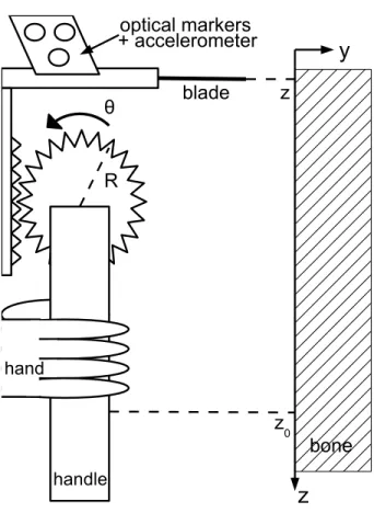
The tool in Figure 1.4 consists of a handle and a blade connected by a gearing mechanism which is actuated by a motor. The goal is to cut in y direction at a desired height zr. The surgeon moves the tool in y direction at a speed v. A deviation from

the desired zr due to a change of bone structure is modeled by a disturbance D acting

along z. In this simple model we assume that the disturbances can make the tool move in z direction only, which means that the tool’s motion is constrained along z except for the cutting motion along y.

z

y

The blade position z is determined by

z= Rθ + z0 (1.1)

and m¨z = F + D + mg (1.2)

where R is the radius of the gear wheel, θ the wheel’s angular position, z0 the handle

position, F the force applied by the gear, m the mass of the subsystem carrying the blade and g is gravity. The motor is governed by

J ¨θ= U − RF

where J is the motor and gear inertia and U the control input. Combining these equations gives ¨ z= U mR+ J/R ´¹¹¹¹¹¹¹¹¹¹¹¹¹¹¹¹¹¹¹¹¹¹¸¹¹¹¹¹¹¹¹¹¹¹¹¹¹¹¹¹¹¹¹¹¹¶ u + D m+ J/R2 + ¨ z0− g 1+ mR2/J ´¹¹¹¹¹¹¹¹¹¹¹¹¹¹¹¹¹¹¹¹¹¹¹¹¹¹¹¹¹¹¹¹¹¹¹¹¹¹¹¹¹¹¹¹¹¹¹¹¹¹¹¹¹¹¹¹¹¹¹¹¹¹¹¹¹¹¹¹¹¹¹¸¹¹¹¹¹¹¹¹¹¹¹¹¹¹¹¹¹¹¹¹¹¹¹¹¹¹¹¹¹¹¹¹¹¹¹¹¹¹¹¹¹¹¹¹¹¹¹¹¹¹¹¹¹¹¹¹¹¹¹¹¹¹¹¹¹¹¹¹¹¹¹¶ d +g . (1.3)

This yields the simplified system

˙z = v (1.4)

˙v= u + d + g . (1.5)

The variable d includes the disturbance D due to bone structure as well as disturbances due to the surgeon motion (modeled by ¨z0).

An optical tracking system measures the position zm = z with a frequency of

1/T = 50Hz at discrete instants zm,k = zm(kT ), an inertial sensor (accelerometer) measures

am= u + d + ab where ab is the accelerometer constant bias.

The inertial measurements are considered continuous because their frequency is much higher than that of the optical ones.

We now present three systems using different types of measurements in a standard servo-control design. In all three cases, we do not take measurement noise into account and l, L, ˜L, h and K are appropriately calculated constant gains. The disturbance d is modeled as a constant:

˙ d= 0 .

System 1 uses only optical measurements zm,k. An observer estimates the state

x= [z, v, d + g]T: prediction: ˙ˆx−₌⎡⎢⎢⎢ ⎢⎢ ⎣ ˆ v− u+ ̂(d + g)− 0 ⎤⎥ ⎥⎥ ⎥⎥ ⎦ =⎡⎢⎢⎢ ⎢⎢ ⎣ 0 1 0 0 0 1 0 0 0 ⎤⎥ ⎥⎥ ⎥⎥ ⎦ ˆ x−+⎡⎢⎢⎢ ⎢⎢ ⎣ 0 1 0 ⎤⎥ ⎥⎥ ⎥⎥ ⎦ u (1.6) correction: ˆxk= ˆx−k+ L(zm,k−1− ˆzk−1) (1.7)

where ˆx− k = ∫

kT

kT−T ˙ˆx−(τ)dτ with ˆx−(kT − T ) = ˆxk−1. The state estimation is used in the

controller which reads

uk= −K ˆxk+ hzr .

This system corresponds to the case where only an optical tracking system is used. System 2 uses both optical and inertial data and represents the setup we propose in Chapter 2. A first observer with state x = [z, v, ab− g]T, measured input am and discrete

optical measurements zm,k reads:

prediction: ˙ˆx−₌⎡⎢⎢⎢ ⎢⎢ ⎣ ˆ v am− ̂(ab− g) − 0 ⎤⎥ ⎥⎥ ⎥⎥ ⎦ =⎡⎢⎢⎢ ⎢⎢ ⎣ 0 1 0 0 0 −1 0 0 0 ⎤⎥ ⎥⎥ ⎥⎥ ⎦ ˆ x−+⎡⎢⎢⎢ ⎢⎢ ⎣ 0 1 0 ⎤⎥ ⎥⎥ ⎥⎥ ⎦ am (1.8) correction: ˆxk= ˆx−k+ L(zm,k−1− ˆzk−1) (1.9) where ˆx− k = ∫ kT

kT−T ˙ˆx−(τ)dτ with ˆx−(kT − T ) = ˆxk−1. This observer gives a continuous

estimation ˆz(t) which is used as a measurement zm(t) for a second observer with state

˜ x= [˜z, ˜v, ˜d+ g]T: ˙ˆ˜x =⎡⎢⎢⎢_⎢⎢ ⎢⎣ ˆ ˜ v ̂ (g + ˜ )d+ u 0 ⎤⎥ ⎥⎥ ⎥⎥ ⎥⎦+ ˜L(z m− ˆ˜z) = ⎡⎢ ⎢⎢ ⎢⎢ ⎣ 0 1 0 0 0 1 0 0 0 ⎤⎥ ⎥⎥ ⎥⎥ ⎦ ˆ ˜ x+⎡⎢⎢⎢ ⎢⎢ ⎣ 0 1 0 ⎤⎥ ⎥⎥ ⎥⎥ ⎦ u+ ˜L(zm− ˆ˜z) (1.10)

This continuous state estimation of the second observer is used in the controller which reads

u= −K ˆ˜x + hzr .

In system 3 which uses optical and inertial data we suppose that tracking and control are more tightly coupled than in system 2. A first observer is used to estimate the disturbance d with inertial measurements am= u + d + ab:

˙ ̂

d+ ab = l(am− u − (̂d+ ab)) (1.11)

This observer gives a continuous estimation ̂d+ ab(t) which is used as input for the second

controller-observer. Its state is x = [z, v, ab−g]T and it uses discrete optical measurements

zm,k: prediction: ˙ˆx−₌⎡⎢⎢⎢ ⎢⎢ ⎣ ˆ v− u+ (̂d+ab) − (̂ab−g)− 0 ⎤⎥ ⎥⎥ ⎥⎥ ⎦ =⎡⎢⎢⎢ ⎢⎢ ⎣ 0 1 0 0 0 −1 0 0 0 ⎤⎥ ⎥⎥ ⎥⎥ ⎦ ˆ x−+⎡⎢⎢⎢ ⎢⎢ ⎣ 0 1 0 ⎤⎥ ⎥⎥ ⎥⎥ ⎦ (u + (̂d+ab)) (1.12) correction: ˆxk= ˆx−k+ L(zm,k−1− ˆzk−1) (1.13)

0 0.5 1 1.5 2 2.5 3 −0.1 −0.05 0 0.05 0.1 0.15 0.2 0.25 z (cm) system 1 system 2 system 3 0 0.5 1 1.5 2 2.5 3 −0.1 −0.05 0 0.05 0.1 0.15 0.2 0.25 z (cm) system 1 system 2 system 3 0 0.5 1 1.5 2 2.5 3 −0.1 −0.05 0 0.05 0.1 0.15 0.2 0.25 z (cm) system 1 system 2 system 3 0 0.5 1 1.5 2 2.5 3 −0.1 −0.05 0 0.05 0.1 0.15 0.2 0.25 z (cm) system 1 system 2 system 3 0 0.5 1 1.5 2 2.5 3 −0.1 −0.05 0 0.05 0.1 0.15 0.2 0.25 z (cm) y (cm) system 1 system 2 system 3 0 0.5 1 1.5 2 2.5 3 0 0.05 0.1 0.15 0.2 d (m/s 2 )

Figure 1.5: Simulation results for the 1D model of a handheld tool, showing the form of the cut for three different servo-control systems in response to a disturbance.

where ˆx− k = ∫

kT

kT−T ˙ˆx−(τ)dτ with ˆx−(kT − T ) = ˆxk−1. The control input is

uk= −K ˆxk+ hzr− (̂d+ ab) .

The handheld tool model and the three servo-control systems were implemented in a Simulink model. Figure 1.5 shows the simulated cuts for these three systems for a desired cutting position zr= 0cm and a disturbance d occurring from t = 2.002s and t = 2.202s. At

a speed of 0.5cm/s, this means the disturbance acts from y = 1.001cm to y = 1.101cm. The disturbance causes the largest and longest deviation in the first system. In system 2, the position deviation can be corrected much faster and its amplitude is much smaller. Using the system 3 can correct the deviation even better. This simulation shows that using inertial sensors with a higher bandwidth allows the servo-control to correct a deviation caused by a disturbance much better than a system with a low bandwidth such as an optical tracking system.

It is important to note that the controller-observer for system 1 cannot be tuned to reject the disturbance faster; the choice of K and L is constrained by the frequency of the optical measurements.

System 1 corresponds to the case in which the existing optical tracking system in a computer-assisted surgery system would be used for a servo-controlled handheld saw without cutting guides. In the following chapters, we will look at an optical-inertial tracking system like the one in system 2. Here, the tracking is independent of the handheld

tool. In system 3, the tracking and servo-control are more tightly coupled. This allows for a even better disturbance rejection than in system 2 but the setup is more complex since the tool’s model has to be known.

1.6

Outline

Optical-Inertial Tracking System The system setup and a mathematical model for the optical-inertial tracking system are described in Chapter 2.

State of the Art An overview of the state of the art of computer vision and optical tracking and of optical-inertial tracking systems is given in Chapter 3. The motivation of several choices for our optical-inertial tracking system as opposed to existing systems are exposed. Calibration methods for the individual sensors and for the hybrid optical-inertial system are discussed in Section 3.3.

Data Fusion Chapter 4 starts by presenting the Extended Kalman Filter (EKF) which is commonly used for data fusion of a nonlinear system and gives two of its variants: the Multiplicative EKF (MEKF) for estimating a quaternion which respects the geometry of the quaternion space and the continuous-discrete EKF for the case of a continuous system model and discrete measurements. Both of these variants are relevant to the considered problem since the Sensor Unit orientation is expressed by a quaternion and because the model for the Sensor Unit dynamics is continuous while the optical measurements are discrete.

The second part of the Chapter presents several data fusion algorithms for the optical-inertial tracking system, starting with an MEKF. Since our goal is to reduce the complexity of the algorithm, other variants are proposed, namely so-called invariant EKFs which exploit symmetries which are present in the considered system. We also discuss a fundamental difference of our data fusion algorithms to those presented in the literature which consists in using optical image data directly as a measurement instead of using triangulated 3D data. We call our approach a "direct" filter as opposed to "indirect" filters using 3D optical data.

The last part of the Chapter is dedicated to the analysis of the influence of parameter errors on one of the invariant EKFs for the optical-inertial system. Using this analysis, we propose a method for calibrating the optical-inertial setup using estimations from the invariant EKF.

Implementation Different aspects of the implementation of an optical-inertial tracking system are studied in Chapter 5. An experimental setup was developed consisting of low-cost cameras from the Wiimote and a Sensor Unit. A microcontroller is used for

synchronized data acquisition from optical and inertial sensors with sample rates of 50Hz and 250Hz respectively. The data fusion algorithm is implemented in Simulink and executed in real-time with an xPC Target application.

Several experiments have been conducted and analyzed to evaluate the performance of the tracking system. They show that the optical-inertial system can track fast motion and does so better than an optical tracking system.

This Chapter also discusses calibration of the individual sensors and of the hybrid setup. It gives the results of several calibration procedures and shows their influence on the tracking performance.

Conclusion To conclude, we give a summary of the work presented in this thesis and an outlook on future work.

1.7

Publications

Part of the work described in this thesis was published in articles at the following conferences:

• Claasen, G., Martin, P. and Picard, F.: Hybrid optical-inertial tracking system for a servo-controlled handheld tool. Presented at the 11th Annual Meeting of the International Society for Computer Assisted Orthopaedic Surgery (CAOS), London, UK, 2011

• Claasen, G. C., Martin, P. and Picard, F.: Tracking and Control for Handheld Surgery Tools. Presented at the IEEE Biomedical Circuits and Systems Conference (BioCAS), San Diego, USA, 2011

• Claasen, G. C., Martin, P. and Picard, F.: High-Bandwidth Low-Latency Tracking Using Optical and Inertial Sensors. Presented at the 5th International Conference on Automation, Robotics and Applications (ICARA), Wellington, New Zealand, 2011

The authors of the above articles have filed a patent application for the optical-inertial tracking with a direct data fusion approach. It has been assigned the Publication no. WO/2011/128766 and is currently under examination.

Chapter 2

Optical-Inertial Tracking System

Ce chapitre présente le système optique-inertiel que nous proposons. Nous expliquons les bases du fonctionnement du système optique et des capteurs inertiels et leurs erreurs et bruits respectifs. La deuxième partie traite du modèle mathématique du système en précisant les coordonnées utilisées, les équations de la dynamique et de sortie et les modèles des bruits.

2.1

System Setup

The goal of this tracking system is to estimate the position and orientation of a handheld object. A so-called Sensor Unit is attached to the object. The Sensor Unit consists of an IMU with triaxial accelerometers and triaxial gyroscopes and optical markers. The IMU and the markers are rigidly fixed to the Sensor Unit. A stationary stereo camera pair is placed in such a way that the optical markers are in its field of view. The setup is depicted in Figure 2.1.

The tracking system uses both inertial data from the IMU and optical data from the cameras and fuses these to estimate the Sensor Unit position and orientation.

This Section presents a few basic elements of the optical system and the inertial sensors which will serve as groundwork for the mathematical model of the system in Section 2.2.

2.1.1

Optical System

Vision systems treat images obtained from a camera, a CT scan or another imaging technique to detect objects, for example by their color or form. In contrast to this, an optical tracking system observes point-like markers which are attached to an object. Instead of treating and transmitting the whole image captured by the camera, they detect only the marker images and output their 2D coordinates.

cameras

optical

markers

servo-controlled

handheld tool

IMU

sensor

unit

C image plane camera/principal axis M m Y X Z u

Figure 2.2: Pinhole camera model

The 2D marker coordinates can then be used to calculate information about the object position. For this, we need to model how a 3D point which represents an optical marker is projected to the camera screen. This Section describes the perspective projection we use and discusses problems and errors which can occur with optical tracking systems.

2.1.1.1 Pinhole Model

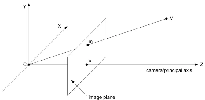
The pinhole model is the standard model for projecting object points to the camera image plane for CCD like sensors [Hartley and Zisserman, 2003, p. 153].

The model is depicted in Figure 2.2 [Hartley and Zisserman, 2003, p. 154]. C is the camera center. u is the principal point. A 3D point is denoted M and its projection in the image plane m. The distance between the camera center and the image plane is the focal distance f.

Figure 2.3 shows the concept of projection as given in [Hartley and Zisserman, 2003, p. 154]. The y coordinate of the image m can be calculated with the theorem of intercepting lines: my Y = f Z ⇔ my = f Y Z

C M m Y Z u f f Y Z Figure 2.3: Projection

mx can be calculated analogously. This gives for the image m:

m= f Z ⎡⎢ ⎢⎢ ⎢⎢ ⎣ X Y Z ⎤⎥ ⎥⎥ ⎥⎥ ⎦

Often, images are expressed in the image plane, in coordinates attached to one corner of the image sensor. In this case, the principal point offset has to be taken into account:

m= [f

X Z + u0

fY_Z + v0] (2.1)

where u = [u0, v0]T is the principal point, expressed in image plane coordinates.

Focal distance and principal point are camera parameters. They are called intrinsic values and have to be determined for each individual camera by a calibration procedure. Projection in homogeneous coordinates Perspective projection for pinhole camera model is often expressed in homogeneous coordinates. In homogeneous coordinates, point M reads ˜M = [X, Y, Z, 1]T and image m reads ˜_m = [m

x, my, 1]T. Point ˜M is

then projected to ˜m by:

˜

where P is the camera matrix. It is equal to P =⎡⎢⎢⎢ ⎢⎢ ⎣ f 0 u0 0 f v0 0 0 1 ⎤⎥ ⎥⎥ ⎥⎥ ⎦ ´¹¹¹¹¹¹¹¹¹¹¹¹¹¹¹¹¹¹¹¹¹¹¹¹¸¹¹¹¹¹¹¹¹¹¹¹¹¹¹¹¹¹¹¹¹¹¹¹¹¶ K [I3 0] (2.3)

The projection (2.2) then writes ˜ m=⎡⎢⎢⎢ ⎢⎢ ⎣ f 0 u0 0 0 f v0 0 0 0 1 0 ⎤⎥ ⎥⎥ ⎥⎥ ⎦ ´¹¹¹¹¹¹¹¹¹¹¹¹¹¹¹¹¹¹¹¹¹¹¹¹¹¹¹¹¹¹¹¹¹¹¹¹¸¹¹¹¹¹¹¹¹¹¹¹¹¹¹¹¹¹¹¹¹¹¹¹¹¹¹¹¹¹¹¹¹¹¹¹¹¶ P ˜ M (2.4) =⎡⎢⎢⎢ ⎢⎢ ⎣ f X+ u0Z f Y + v0Z Z ⎤⎥ ⎥⎥ ⎥⎥ ⎦ = Z⎡⎢⎢⎢ ⎢⎢ ⎣ f X/Z + u0 f Y/Z + v0 1 ⎤⎥ ⎥⎥ ⎥⎥ ⎦ = Z [m_{1 ]} (2.5)

The image m can then be retrieved from the homogeneous image ˜m. The image is expressed in the image plane as in Equation (2.1).

The matrix K is called the intrinsic matrix. If f and [u0, v0] are given in pixels,

the projected image will be in pixels. If the pixels are not square, the aspect ration a which describes the relation between the width and height of a pixel has to be taken into account: K =⎡⎢⎢⎢ ⎢⎢ ⎣ f 0 u0 0 af v0 0 0 1 ⎤⎥ ⎥⎥ ⎥⎥ ⎦

Alternatively, two focal lengths fx and fy for the sensor x and y dimensions can be used

instead of the common focal length f [Szeliski, 2011, p. 47]. The intrinsic matrix K then writes K =⎡⎢⎢⎢ ⎢⎢ ⎣ fx 0 u0 0 fy v0 0 0 1 ⎤⎥ ⎥⎥ ⎥⎥ ⎦

In this model, skew and lens distortion are not taken into account.

The values of the intrinsic matrix are usually determined for a individual camera by a calibration procedure as described in Section 3.3.1.

2.1.1.2 Noise/Error Sources

The image data measured by a camera can be corrupted by measurement noise and quantization noise where the latter depends on pixel size and resolution. When point images are considered, they may contain segmentation or blob detection errors.

For projection using the pinhole model, errors in the intrinsic values cause errors in the projected image.

2.1.2

Inertial Sensors

Inertial sensors designate accelerometers and gyroscopes which measure specific accelera-tion resp. angular rate without an external reference [Groves, 2008, p. 97].

An accelerometer measures specific acceleration along its sensitive axis. Most accelerometers have either a pendulous or a vibrating-beam design [Groves, 2008, p. 97]. A gyroscope measures angular rate about its sensitive axis. Three types of gyroscopes can be found which follow one of the three following principles: spinning mass, optical, or vibratory [Groves, 2008, p. 97].

Inertial sensors vary in size, mass, performance and cost. They can be grouped in five performance categories: marine-grade, aviation-grade, intermediate-grade, tactical-grade, automotive grade [Groves, 2008, p. 98].

The current development of inertial sensors is focused on micro-electro-mechanical systems (MEMS) technology. MEMS sensors are small and light, can be mass produced and exhibit much greater shock tolerance than conventional designs [Groves, 2008, p. 97]. An inertial measurement unit (IMU) consists of multiple inertial sensors, usually three orthogonal accelerometers and three orthogonal gyroscopes. The IMU supplies power to the sensors, transmits the outputs on a data bus and also compensates many sensor errors [Groves, 2008].

2.1.2.1 Noise/Error Sources

Several error sources are present in inertial sensors, depending on design and performance category. The most important ones are

• bias

• scale factor

• misalignment of sensor axes • measurement noise

Each of the first three errors source has four components: a fixed term, a temperature-dependent variation, a run-to-run variation and an in-run variation [Groves, 2008]. The fixed and temperature-dependent terms can be corrected by the IMU. The run-to-run variation changes each time the IMU is switched but then stays constant while it is in use. The in-run variation term slowly changes over time.

Figure 2.4: Sample plot of Allan variance analysis results from [IEEE, 1997] Among the error sources listed above, bias and measurement noise are the dom-inant terms while scale factors and misalignment can be considered constant and can be corrected by calibration [Gebre-Egziabher, 2004, Gebre-Egziabher et al., 2004, Groves, 2008]. Bias and measurement noise for inertial sensor noise are often de-scribed using the Allan variance [Allan, 1966]. The Allan variance is calculated from sensor data collected over a certain length of time and gives power as a function of averaging time (it can be seen as a time domain equivalent to the power spectrum) [Gebre-Egziabher, 2004, Gebre-Egziabher et al., 2004]. For inertial sensors, different noise terms appear in different regions of the averaging time τ [IEEE, 1997] as shown in Figure 2.4 for a gyroscope. The main noise terms are the angle random walk, bias instability, rate random walk, rate ramp and quantization noise.

Since the Allan variance plots of the gyroscopes used in the implementation in Section 5 (see Section 5.1.5.3 for details on the noise parameters used in the implementation) can be approximated using only the angle random walk (for the measurement noise) and rate random walk (for the time-variation of the bias), we will use only these two terms in the gyroscope models presented in the following Section. The angle random walk corresponds to the line with slope -1/2 and its Allan variance is given [IEEE, 1997] as

σ2(τ) = N

2

τ

where N is the angle random walk coefficient. The rate random walk is represented by the line with slope +1/2 and is given [IEEE, 1997] as

σ2(τ) = K

2_τ

where K is the rate random walk coefficient.

The accelerometer error characteristics can be described analogously to the gyroscope case, also using only two of the terms in the Allan variance plot. We will consider that possible misalignment and scale factors have been compensated for in the IMU or by a calibration procedure.

2.2

Mathematical Model

2.2.1

Coordinate systems

The motion of the Sensor Unit will be expressed in camera coordinates which are denoted by C and are fixed to the right camera center. C_v is a velocity in camera coordinates,

for example. The camera frame unit vectors are E1 = [1, 0, 0]T, E2 = [0, 1, 0]T and

E3= [0, 0, 1]T. The camera’s optical axis runs along E1. Image coordinates are expressed

in the image sensor coordinate system S which is attached to one of the corners of the camera’s image sensor.

The left camera coordinate system is denoted by CL and the image sensor coordinate system by SL. The left camera unit vectors are ˜E1, ˜E2 and ˜E3. Coordinates C and CL

are related by a constant transformation.

The body coordinates, denoted by B, are fixed to the origin of the IMU frame and are moving relative to the camera frames. B_a is an acceleration in body coordinates, for

example.

The optical markers are defined in marker coordinates M. Marker and body coordinates are related by a constant transformation.

Finally, we also use an Earth-fixed world coordinate system, denoted by W .

The different frames are depicted in Figure 2.5. Figure 2.6 shows the image sensor and its frames in detail.

2.2.2

Quaternions

A quaternion q [Stevens and Lewis, 2003] consists of a scalar q0∈ R and a vector ˜q ∈ R3:

q= [q0, ˜qT]T .

The quaternion product of two quaternions s and q is defined as s∗ q = [ s0q0− ˜s˜q

s0q˜+ q0s˜+ ⃗s× ˜q]

. The cross product for quaternions reads:

s× q = 1

C

_Z

_Y

_X

u

v

f

_Y

_X

_Z

_Y

_X

camera image sensor

sensor unit

_Y

_X

_Z

IMU

_Y

_X

_Z

S

_y

_x

_z

_y

_x=f

u

v

camera image sensor

A unit quaternion can be used to represent a rotation: R(q)a = q ∗ a ∗ q−1

where a ∈ R3 and R(q) is the rotation matrix associated with quaternion q. If q depends

on time, we have ˙q−1_{= −q}−1_{∗ ˙q ∗ q}−1_{. If}

˙

q= q ∗ a + b ∗ q (2.6)

with a,b ∈ R3 holds true, then ∥q(t)∥ = ∥q(0)∥ for all t.

2.2.3

Dynamics Model

We have three equations representing the Sensor Unit motion dynamics:

C_p˙=C_{v (2.7)}

C_˙v=C_G+BC_q∗B_a∗BC_q−1 _(2.8) BC_q˙= 1

2

BC_q∗B_{ω (2.9)}

where C_G = W C_q∗W_G∗W C_q−1 is the gravity vector expressed in camera coordinates. W_G= [0, 0, g]T is the gravity vector in the world frame with g = 9.81m

s2 and W Cq describes

the (constant) rotation from world to camera coordinates. C_p andC_v are the Sensor Unit

position and velocity, respectively. The orientation of the Sensor Unit with respect to camera coordinates is represented by the quaternionBC_q. B_aand B_ω are the Sensor Unit

accelerations and angular velocities.

2.2.4

Output Model

To project the markers to the camera we use the standard pinhole model from (2.1) but rewrite it using scalar products:

C_y i = f ⟨C_m i,CE1⟩ [⟨Cmi,CE2⟩ ⟨C_m i,CE3⟩] (2.10) with C_m i=Cp+BCq∗Bmi∗BCq−1

where yi is the 2D image of marker i with i = 1, . . . , l (l is the number of markers). f is

the camera’s focal distance. To simplify notations, we use only one common focal length; if pixels are not square (see Section 2.1.1), we should write diag(f, af) instead of f. C_m

i

andB_m

i are the position of marker i in camera and body coordinates, respectively. ⟨a, b⟩

The 2D image can be transformed from camera to sensor coordinates by a translation:

S_y

i=Cyi+Su

where S_u is the camera principal point.

The camera coordinate system in which the Sensor Unit pose is expressed is assumed to be attached to the right camera of the stereo camera pair. The transformation between the left and right camera coordinates is expressed by RSt and tSt:

CL_{p= R}

StCp+ tSt (2.11)

To project a marker to the left camera, replace C_m

i in (2.10) by CL_m

i= RStCmi+ tSt (2.12)

and use corresponding parameters and unit vectors:

CL_y i = fL ⟨CL_m i,CLE˜1⟩ [⟨CLmi,CLE˜2⟩ ⟨CL_m i,CLE˜3⟩] . (2.13)

2.2.5

Noise Models

2.2.5.1 Inertial Sensor Noise Models

The noise models are motivated in Section 2.1.2.1 and will now be described mathemati-cally as part of the dynamics model.

The gyroscope measurement ωm is modeled as

ωm=Bω+ νω+Bωb

where ωm is the gyroscope measurement, Bω is the true angular rate, νω is the

measurement noise andB_ω

b is the gyroscope bias. Note that the parameter νωcorresponds

to the angle random walk coefficient N in the Allan variance in Section 2.1.2.1. The gyroscope bias B_ω

b can be represented by a sum of two components: a constant

one and a varying one. The bias derivative depends on the varying component which is modeled as a random walk as described in Section 2.1.2.1:

B_ω˙

b= νωb . (2.14)

Note that the parameter νωb corresponds to the rate random walk coefficient K in the

Allan variance in Section 2.1.2.1.

A more complex noise model is proposed in [Gebre-Egziabher et al., 2004, Gebre-Egziabher, 2004] which also models the variation of the time-varying part of the

10−1 100 101 102 103 104 10−2 10−1 100 101 τ (s)

root Allan variance

angle random walk rate random walk Gauss−Markov

angle RW + rate RW + Gauss−Markov angle RW + rate RW

Figure 2.7: Allan variance for a hypthetical gyroscope

bias with an additional parameter. The bias ωb is written as the sum of the constant

part ωb0 and the time-varying part ωb1:

ωb = ωb0+ ωb1 .

ωb1 is modeled as a Gauss-Markov process:

˙ ωb1= −

ωb1

τ + νωb1

where τ is the time constant and νωb1 the process driving noise. This model contains three

parameters and the Allan variance is approximated by three terms as shown in Figure 2.7. We use a special case of this model with τ = ∞ which simplifies the model but still gives a reasonable approximation in the interval of the Allan variance which we considered and which is given in the inertial sensor datasheet used in the implementation as described in Section 5.1.5.3. The approximated Allan variance with τ = ∞ is illustrated in Figure 2.7.

The accelerometer model is of the same form as the gyroscope model: am=Ba+ νa+Bab

where B_a is the true specific acceleration, ν

a is the measurement noise and Bab is the

accelerometer bias. Note that the parameter νa corresponds to the velocity random walk

coefficient N in the Allan variance in Section 2.1.2.1. The accelerometer biasB_a

bcan be represented by a sum of two components: a constant

one and a varying one. The bias derivative depends on the varying component which is modeled as a random walk as described in Section 2.1.2.1:

B_˙a

b = νab (2.15)

Note that the parameter νab corresponds to the velocity random walk coefficient K in the

Allan variance in Section 2.1.2.1.

Since the IMU consists of a triad of identical accelerometers and a triad of identical gyroscopes and since we consider the inertial sensor noises to be independent white noises with zero mean, we can write for the auto-covariance

E(νj(t)νjT(t + τ)) = ξj2I3δ(τ) (2.16)

for j ∈ {a, ω, ab, ωb}.

2.2.5.2 Camera Noise Model

The marker images are measured in the sensor frame and are corrupted by noise ηy:

ym = [ S_y

SL_{y] +}ηy .

We use the simplest possible noise model which assumes the noise to be white. The camera noise is not actually white but the camera which will be used in the experimental setup in Section 5.1 does not have a datasheet. Thus we do not have any information about its noise characteristics which could permit us to model the noise realistically. Also, we consider that the camera noise model is not critical for the performance of the data fusion algorithms which will be presented in Section 4.3. However, it is important to use a correct noise model for the inertial sensors because these are used in the prediction steps of the data fusion algorithm.

2.2.6

Complete Model

The complete model with noises then reads:

C_p˙=C_{v (2.17)} C_˙v=C_G+BC_{q∗ (a} m− νa−Bab) ∗BCq−1 (2.18) BC_q˙= 1 2 BC_{q∗ (ω} m− νω−Bωb) (2.19) B_˙a b= νab (2.20) B_ω˙ b= νωb . (2.21)

The outputs for the right and the left camera:

S_y i = fR ⟨C_m i,CE1⟩ [⟨Cmi,CE2⟩ ⟨C_m i,CE3⟩] + S_u R (2.22) SL_y i = fL ⟨CL_m i,CLE˜1⟩ [⟨CLmi,CLE˜2⟩ ⟨CL_m i,CLE˜3⟩ ] +SL_u L (2.23)

where i = 1, . . . , l. Indices R and L refer to right and left camera resp. (e.g. fL is the focal

distance of the left camera). The measured outputs are:

yim=Syi+ ηyi (2.24)

y_(i+l)m=SLyi+ ηy(i+l) . (2.25)

The six accelerometer and gyroscope measurements u= [am, ωm]

are considered as the inputs of our system and the marker images y= [Sy1, . . . ,Syl ´¹¹¹¹¹¹¹¹¹¹¹¹¹¹¹¹¹¹¹¹¹¹¹¹¸¹¹¹¹¹¹¹¹¹¹¹¹¹¹¹¹¹¹¹¹¹¹¹¹¶ S_y ,SLy1, . . . ,SLyl ´¹¹¹¹¹¹¹¹¹¹¹¹¹¹¹¹¹¹¹¹¹¹¹¹¹¹¹¹¹¹¹¹¹¸¹¹¹¹¹¹¹¹¹¹¹¹¹¹¹¹¹¹¹¹¹¹¹¹¹¹¹¹¹¹¹¹¹¶ SL_y ]

as its outputs. y is a vector of length 2l+2l = 4l. The state vector which is to be estimated by the data fusion filter in Chapter 4 is of dimension 16 and has the form:

x= [C_p,C_v,BC_q,B_a

b,Bωb] .

This system is observable with l = 3 or more markers. This is a condition for this model to be used in an observer/data fusion algorithm as the ones presented in Chapter 4. See Section 4.3.1 for an observability analysis.

Chapter 3

State of the Art

La présentation de l’état de l’art comporte trois volets: la vision par ordinateur et le tracking optique, le tracking optique-inertiel, et enfin le calibrage.

Dans le volet vision par ordinateur et tracking optique, nous abordons des méthodes pour déterminer la position et l’orientation d’un point ou d’un objet à partir d’images d’un système de caméra monoculaire ou stéréo. Ces méthodes seront utilisées pour le calibrage des caméras et comme référence pour le tracking optique-inertiel.

Des systèmes de tracking utilisant des capteurs optiques et inertiels présentés dans la litérature sont décrits dans la deuxième partie. Ici, nous donnons la motivation de notre approche pour le tracking optique-inertiel et indiquons les différences par rapport aux systèmes existants.

Finalement, nous traitons la question du calibrage des caméras, des capteurs inertiels et du système optique-inertiel.

3.1

Computer Vision and Optical Tracking

Optical tracking uses optical markers attached to an object and one or more cameras which look at these markers. With a camera model and several camera parameters, it is possible to calculate the object position and/or orientation from the marker images, depending on the setup used. The camera model used here is the pinhole model presented in Section 2.1.1.1.

The markers can be active or passive. Active markers send out light pulses. Passive markers are reflecting spheres which are illuminated by light flashes sent from the camera housing [Langlotz, 2004]. The markers are attached to a rigid body which is fixed to the object being tracked. Often, infrared (IR) light and infrared filters are used to simplify marker detection in the images.

Examples of commercially available optical tracking systems are: Optotrak, Polaris (both Northern Digital Inc., Waterloo, Canada [NDI, 2011]), Vicon (Vicon Motion Systems Limited, Oxford, United Kingdom [Vicon, 2011]) and ARTtrack (advanced realtime tracking GmbH, Weilheim, Germany [advanced realtime tracking GmbH, 2011]). The field of computer vision provides algorithms for calculating an object’s position and orientation from the marker images. Here we look into monocular and stereo tracking which use one and two cameras respectively. For monocular tracking, at least four coplanar markers have to be attached to the object to determine the object position and orientation. In stereo tracking, the 3D marker position can be determined from a single marker with a method called triangulation presented in Section 3.1.2.1. In order to calculate an object’s orientation, at least 3 non-collinear markers are needed. Calculating the the object position and orientation from the three triangulated markers is called the "absolute orientation problem" and is discussed in Section 3.1.2.2. While the monocular setup is simpler and does not need synchronization between cameras, it only has a poor depth precision. Stereo tracking is the most common setup for optical tracking systems.

Although the optical-inertial tracking system we propose does not use any of these computer vision algorithms which can be computationally complex we study these algorithms here for several reasons. Monocular tracking is the basis of the camera calibration procedure implemented in the Camera Calibration Toolbox [Bouguet, 2010] and used for calibrating the cameras in the experimental setup in chapter 5 which led us to study this method. Wanting to show that the proposed optical-inertial tracking system is more suitable for following fast motion than an optical tracking system, we examined stereo tracking algorithms to calculate pose using only optical data from our experimental setup. This permits us to compare pose estimation from our optical-inertial system to that of a purely optical system in Section 5.3.

3.1.1

Monocular Tracking

With a single camera, it is possible to calculate position and orientation of a rigid body with four non-collinear points lying in a plane. Using less then four markers or four nonplanar markers does not yield a unique solution while five markers in general positions yield two solutions. To obtain a unique solution at least six markers in general positions have to be fixed to the object. The problem of determining an object position depending on the number and configuration of markers has been called the "Perspective-n-point problem" where n is the number of markers and the solution was given in [Fischler and Bolles, 1981].

We use the setup and frame notations as presented in Figure 2.5 and Section 2.2.1. The four marker points are known in marker coordinates and we define the object position as the origin of the marker frame. The position of marker i in camera coordinates then

reads

C_m

i =M CRMmi+M Ct for i = 1, ..., 4

where the rotation M C_R and the translation M C_t represent the object pose. M_m

i is the

position of marker i and the M_m

i with i = 1, ..., 4 are called the marker model. The goal

is to determine the object pose from the camera imagesS_y i.

Images and marker model are related by

S_y˜

i= KCmi = K[M CRM Ct]Mm˜i

where we have used homogeneous coordinates (see Section 2.1.1.1). Since we have a planar rigid body, the marker coordinates read

M_m

i= [MXi,MYi, 0]T

and we can write the homogeneous marker model as

M_m˜

i,2D= [MXi,MYi, 1]T

This makes it possible to calculate the homography matrix H between markers and images:

S_y˜

i= HMm˜i,2D . (3.1)

The solution presented here first calculates the homography matrix H between markers and images and then determinesM C_tandM C_Rusing H and the camera intrinsic matrix K.

Solving for homography H between model and image This calculation fol-lows [Zhang, 2000] for the derivation of the equations and [Hartley and Zisserman, 2003, ch. 4.1] for the solution for H.

We note the homography matrix:

H =⎡⎢⎢⎢ ⎢⎢ ⎣ hT 1 hT 2 hT 3 ⎤⎥ ⎥⎥ ⎥⎥ ⎦ .

and the homogeneous image:

S_y˜

i = [u, v, 1]T .

Equation (3.1) gives us:

S_y˜ i× H ⋅Sm˜i,2D= ⎡⎢ ⎢⎢ ⎢⎢ ⎣ ui vi 1 ⎤⎥ ⎥⎥ ⎥⎥ ⎦ ×⎡⎢⎢⎢ ⎢⎢ ⎣ hT 1Sm˜i,2D hT 2Sm˜i,2D hT 3Sm˜i,2D ⎤⎥ ⎥⎥ ⎥⎥ ⎦ =⎡⎢⎢⎢ ⎢⎢ ⎣ vihT3Sm˜i,2D− hT2Sm˜i,2D hT 1Sm˜i,2D− uihT3Sm˜i,2D uihT2Sm˜i,2D− vihT1Sm˜i,2D ⎤⎥ ⎥⎥ ⎥⎥ ⎦ = 0

Since only two of the three equations above are linearly independent, each marker i contributes two equations to the determination of H. We omit the third equation and use hT

i Sy˜i,2D=Sy˜ T

i,2Dhi to rewrite the first two equations:

[M˜i,2DT 0 −uiM˜i,2DT

0 M˜T i,2D −viM˜i,2DT ] ´¹¹¹¹¹¹¹¹¹¹¹¹¹¹¹¹¹¹¹¹¹¹¹¹¹¹¹¹¹¹¹¹¹¹¹¹¹¹¹¹¹¹¹¹¹¹¹¹¹¹¹¹¹¹¹¹¹¹¹¹¹¹¹¹¹¹¹¹¹¹¹¹¹¹¹¹¹¹¹¹¹¹¹¹¹¸¹¹¹¹¹¹¹¹¹¹¹¹¹¹¹¹¹¹¹¹¹¹¹¹¹¹¹¹¹¹¹¹¹¹¹¹¹¹¹¹¹¹¹¹¹¹¹¹¹¹¹¹¹¹¹¹¹¹¹¹¹¹¹¹¹¹¹¹¹¹¹¹¹¹¹¹¹¹¹¹¹¹¹¹¹¶ Ai ⋅⎡⎢⎢⎢ ⎢⎢ ⎣ h1 h2 h3 ⎤⎥ ⎥⎥ ⎥⎥ ⎦ ± h = 0

Matrix Ai is of dimension 2 × 9. The four matrices Ai are assembled into a single matrix

A of dimension 8 × 9.

The vector h is obtained by a singular value decomposition of A. The unit singular vector corresponding to the smallest singular value is the solution h which then gives matrix H. Note that H is only determined up to a scale.

The estimation of H can be improved by a nonlinear least squares which minimizes the error between the measured image points S_y

i and the projection Syˆi of the marker

coordinates using the homography H. The projection reads

S_yˆ i= 1 hT 3Mm˜i,2D [hT1Mm˜i,2D hT 2Mm˜i,2D ] The cost function which is to be minimized with respect to H is

∑

i

∥S_y

i−Syˆi∥ .

Closed-form solution for pose from homography and intrinsic matrix Having determined matrix H up to a scale, we can write

sSy˜i= HMm˜i,2D (3.2)

where s is a scale. The homogeneous image can be expressed as

S_y˜ i= K [M CR M Ct]Mm˜i = K [r1 r2 r3 M Ct] ⎡⎢ ⎢⎢ ⎢⎢ ⎢⎢ ⎣ M_X i M_Y i 0 1 ⎤⎥ ⎥⎥ ⎥⎥ ⎥⎥ ⎦ (3.3) = K [r1 r2 M Ct] ⎡⎢ ⎢⎢ ⎢⎢ ⎣ M_X i M_Y i 1 ⎤⎥ ⎥⎥ ⎥⎥ ⎦ ´¹¹¹¹¹¹¹¸¹¹¹¹¹¹¹¶ ˜ mi,2D (3.4)

where K is the intrinsic matrix. With (3.2) and (3.4) we can then write λ[h∗₁ h∗₂ h∗₃]

´¹¹¹¹¹¹¹¹¹¹¹¹¹¹¹¹¹¹¹¹¹¹¹¹¹¹¹¹¹¹¸¹¹¹¹¹¹¹¹¹¹¹¹¹¹¹¹¹¹¹¹¹¹¹¹¹¹¹¹¹¹¹¶

H

= K [r1 r2 M Ct]

where λ is an arbitrary scale and h∗

j are the columns of matrix H. This gives:

r1 = λK−1h∗1 (3.5)

r2 = λK−1h∗2 (3.6)

r3 = r1× r2 (3.7)

M C_{t= λK}−1_h∗

3 (3.8)

Theoretically, we should have

λ= 1

∥K−1_h∗ 1∥

= _∥K−11 h∗₂∥

but this is not true in presence of noise. [DeMenthon et al., 2001] proposes to use the geometric mean to calculate λ:

λ= √ 1 ∥K−1_h∗ 1∥ ⋅_∥K−11 h∗₂∥ (3.9) Matrix M C_R = [r

1 r2 r3] is calculated according to (3.5)–(3.7) and M Ct according

to (3.8), using the scale λ given in (3.9).

3.1.2

Stereo Tracking

3.1.2.1 Triangulation

Knowing the camera intrinsic parameters, a marker image point can be back-projected into 3D space. The marker lies on the line going through the marker image and the camera center but its position on this line cannot be determined. When two cameras are used, the marker position is determined by the intersection of the two back-projected lines. This concept is called triangulation.

However, these two lines only intersect in theory. In the presence of noise (and due to inaccurate intrinsic parameters), the two back-projected lines will not intersect. Several methods have been proposed to estimate the marker position for this case. The simplest one is the midpoint method [Hartley and Sturm, 1997] which calculates the midpoint of the common perpendicular of the two lines. In the comparison presented in [Hartley and Sturm, 1997] the midpoint method gives the poorest results. This is