A multi-sensor, cable-driven parallel manipulator based lower limb rehabilitation device : design and analysis

(1)

HAL Id: pastel-00933732

https://pastel.archives-ouvertes.fr/pastel-00933732

Submitted on 21 Jan 2014

HAL is a multi-disciplinary open access

archive for the deposit and dissemination of sci-entific research documents, whether they are pub-lished or not. The documents may come from teaching and research institutions in France or abroad, or from public or private research centers.

L’archive ouverte pluridisciplinaire HAL, est destinée au dépôt et à la diffusion de documents scientifiques de niveau recherche, publiés ou non, émanant des établissements d’enseignement et de recherche français ou étrangers, des laboratoires publics ou privés.

A multi-sensor, cable-driven parallel manipulator based

lower limb rehabilitation device : design and analysis

Mandar Harshe

To cite this version:

Mandar Harshe. A multi-sensor, cable-driven parallel manipulator based lower limb rehabilitation device : design and analysis. Other [cs.OH]. Ecole Nationale Supérieure des Mines de Paris, 2012. English. �NNT : 2012ENMP0102�. �pastel-00933732�

(2)

T

H

È

S

E

INSTITUT DES SCIENCES ET TECHNOLOGIES

École doctorale n

O

84 :

Sciences et technologies de l’information et de la communication

Doctorat ParisTech

T H È S E

pour obtenir le grade de docteur délivré par

l’École nationale supérieure des mines de Paris

Spécialité « Informatique temps réel, robotique et automatique »

présentée et soutenue publiquement par

Mandar Harshe

le 21 décembre 2012

Analyse et conception d’un système de rééducation de membres

inférieurs reposant sur un robot parallèle à câbles

A multi-sensor, cable-driven parallel manipulator based lower limb

rehabilitation device : design and analysis

Directeur de thèse : Jean-Pierre MERLET Jury

M. Philippe GORCE,

Professeur, HandiBio, Univ. du Sud Toulon-Var Rapporteur M. Lotﬁ ROMDHANE,

Professeur, Laboratoire de Mécanique de Sousse, Ecole Nationale d’Ingenieurs de Sousse Rapporteur M. Jean-Pierre MERLET,

Directeur de recherche, COPRIN, INRIA Sophia Antipolis Examinateur M. Vincenzo PARENTI CASTELLI,

Professeur, Department of Mechanical Engineering , University of Bologna Examinateur M. Mohamed BOURI,

Group Leader, LSRO, Ecole Polytechnique Fédérale de Lausanne Examinateur MINES ParisTech

COPRIN, INRIA Sophia Antipolis

(3)

(4)

(5)

(6)

Acknowledgements

I would like to begin by thanking my thesis director, Dr. Jean-Pierre Merlet, for giving me an opportunity to pursue my doctoral research at the COPRIN research team at INRIA Sophia An-tipolis. I am extremely grateful for his guidance, supervision, advice, encouragement and support, which has aided me immensely in completing this work. I am grateful for his confidence in my abili-ties and am certain that the skills I gained while working with him will be invaluable in my future work. I am also extremely grateful to David Daney for his guidance in various topics, both technical and non-technical. He provided me an informal sounding board off of which I could bounce my ideas. I immensely benefited from the long discussions we had which helped me fine-tune some of my vague ideas into working solutions.

I am also thankful for Mr. Vincenzo Parenti Castelli, and Mr. Mohamed Bouri who agreed to be the jury for my thesis defense. I am grateful for the comments of my reviewers Mr. Lotﬁ Romdhane and Mr. Philippe Gorce and for their suggestions to improve this thesis.

I would also like to thank Michael Burman, Sami Bennour and Haibo Qu for their help in my research. Michael and Sami were instrumental in helping me set up the initial stages of our experi-ments and their contributions are greatly appreciated. Sami and Haibo also kindly agreed to aid and be a part of the experimental trials, for which I am indebted.

Working with the COPRIN research team has been an immense pleasure and I am thankful to the team for their help not only in my research, but also in navigating various aspects of moving to a new country, learning the language and living in France. Our meandering lunch time conversa-tions are something I will miss as well. I would particularly like to thank Gilles Trombettoni for his impromptu lunchtime French lessons, and Christine Claux and Nathalie Woodward for their admin-istrative help. Thanks also go to other members of the team - Odile Pourtallier, Bertrand Niveau, Yves Papegay and Nicolas Chleq. I am incredibly thankful to my fellow doctoral students and col-leagues Julien Hubert, Guillaume Aubertine, Thibault Gayral, Julien Alexandre dit Sandretto, Remy Ramadour and Laurent Blanchet for the great times, both in and out of the lab; for helping me ease into life in France, translating numerous emails and phone conversations and for teaching me French. I would be remiss if I did not acknowledge the help and support I have received from friends and ﬂatmates in the last three years. For helping create a home away from home, I thank my current and previous ﬂatmates. A great big thank you to all friends I have gotten to know in and outside France for all the good times, help, anecdotes, adventures, hikes, accidents, and laughter, in no particular order: André, Andres, Oscar, Rubiela, Michael, Miguel, Marie-Anne, Yann, Quentin, Jean-Daniel, Olivier, Maria, Ashwin, Cyril, Bethany, Anjalee, Priyank, Vishesh, Dori, Erick, Anais, Anna, Marcos, Cecile, Angelo, Nikhil and Abhishek.

Finally, I am indebted to my family for their love and support. My parents and my sister have supported me in all my decisions and have spared no eﬀort in ensuring that I get the best opportunities to succeed. Seeing their son leave for another country must have been much more diﬃcult for my

(7)

vi

parents than I could imagine and I am grateful for their unwavering support. Thank you all for your contributions, great and small, to this ﬁnished work. I couldn’t have done it without you.

(8)

List of Figures

1.1 A motion capture system for gait analysis . . . 3

1.2 Right knee . . . 3

1.3 Contact point variation in knee . . . 5

1.4 Magnetic Resonance Imaging of the loaded knee . . . 6

1.5 Typical knee gait analysis . . . 6

1.6 A typical serial robot (SCARA) . . . 9

1.7 Cable driven parallel robots at INRIA . . . 10

1.8 The Romer portable CMM . . . 10

1.9 The ARMin exoskeleton for arm rehabilitation . . . 11

1.10 The Lokomat gait training system . . . 11

1.11 The Active Leg EXoskeleton . . . 12

1.12 The Ekso . . . 12

1.13 Rehabilitation robots at EPFL . . . 12

1.14 Ankle rehabilitation robots . . . 13

1.15 The NeReBot . . . 14

1.16 The String-Man robot conﬁguration . . . 14

2.1 The ISB recommendations for coordinate systems for the human body segments . . . 19

2.2 The classical knee-joint coordinate system . . . 19

2.3 Collars used in the experiment . . . 22

3.1 The MARIONET-REHAB frame . . . 28

3.2 The pulley arrangement on the actuated cable-based parallel robot . . . 28

3.3 A CAD model of the MARIONET-REHAB . . . 29

3.4 The passive wire sensors on the frame . . . 29

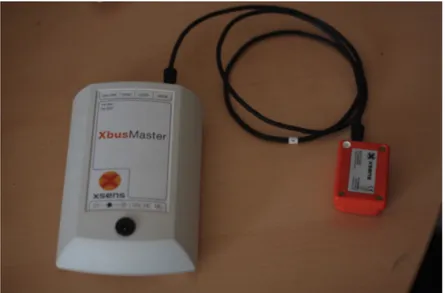
3.5 The XBus Master along with a MTx inertial measurement unit . . . 30

3.6 The Phidget accelerometer, which may be added to the collar . . . 30

3.7 MTx sensor with sensor-ﬁxed coordinate system S . . . 32

3.8 Optical motion capture system . . . 34

3.9 A pressure sensor with the Data Cuﬀ . . . 35

3.10 Pressure distribution after right heel strike . . . 35

3.11 Collar force sensors . . . 36

3.12 IR reﬂective sensors . . . 36

4.1 Collar calibration . . . 38

4.2 Coordinate systems for Hayati’s convention . . . 39

4.3 Model of collar components . . . 40

4.4 Plate frames and transformation matrices . . . 41

4.5 Unprocessed Position Data from Optical Markers . . . 47

4.6 Search space for new point in track . . . 48

4.7 Cleaned Position Data from Optical Markers . . . 48

4.8 Plot of femoral collar hinge angles as estimated by the EKF . . . 49

(11)

x LIST OF FIGURES

5.1 Subject ﬁtted with sensors, ready for experimental trials . . . 56

5.2 Accelerometer raw data . . . 57

5.3 Fourier transform of the accelerometer data along x-axis . . . 58

5.4 Fourier transform of the passive wire data (for wire 1) . . . 58

5.5 Passive wire length raw data . . . 59

5.6 Passive wire length data, passed through low-pass ﬁlter . . . 59

5.7 Active wire data, with low noise . . . 59

5.8 Noisy position data for marker on tibia . . . 60

5.9 Femoral collar joint angles . . . 62

5.10 Lower tibial collar joint angles . . . 62

5.11 Tibial collar joint angles, shown separately . . . 62

5.12 DistancePt1Pt4 . . . 63

5.13 DistancePt1Pt4, Second trial . . . 64

5.14 Tibial collar joint angles for second trial, shown separately . . . 65

(12)

List of Tables

2.1 Sensor Data available . . . 24

4.1 Identiﬁed parameters for ﬁrst plate of the three collars . . . 43

4.2 Fixed parameters for femoral collar . . . 44

4.3 Fixed parameters for lower tibial collar . . . 44

4.4 Fixed parameters for upper tibial collar . . . 44

5.1 Collars used in experiment . . . 54

5.2 Sensor distribution over collars . . . 54

(13)

(14)

1 Introduction

Résumé

Au sein de ce chapitre, nous évoquons les enjeux mondiaux des politiques de santé pour les prochaines 50 années. Notre propos porte sur les questions de mobilité soulevées par l’augmentation de la proportion de la population âgée de plus de 60 ans. Nous mettons en évidence les problèmes et les maladies concernant l’articulation du genou. Aﬁn de bien cerner ces problèmes du genou, nous introduisons les méthodes d’analyse de la marche, étudions la physiologie du genou et identiﬁons les avantages et inconvénients des méthodes modélisant l’articulation du genou.

Nous commençons ce chapitre par une discussion sur l’analyse de la marche et une de-scription du mouvement du genou, tel qu’il est présenté dans les premiers travaux sur les cadavres humains. Nous présentons ensuite plusieurs méthodes utilisant différentes technolo-gies d’imagerie - IRM, CT-scan et radiographie -, lesquelles fournissent des informations sur le modèle statique du genou. Pour étudier le mouvement dynamique du genou, nous devons considérer l’effet des artefacts de tissus « mous ». Ces considérations nous conduisent vers différents types de méthodes : certaines utilisant des procédés de capture optique, d’autres des capteurs inertiels, des capteurs magnétiques, des capteurs à ultrasons, ou encore utilisant des capteurs de force plantaire. Ce chapitre nous présente donc un aperçu de ces méthodes, étudiant leurs avantages et inconvénients.

Nous présentons également au sein de ce chapitre quelques exemple de systèmes de rééducation robotiques, considérant leurs spéciﬁcités concernant la physiologie du genou, ainsi que des critères de modularité, simplicité et précision. Nous pouvons dès lors introduire le robot MARIONET-REHAB, développé au sein de notre laboratoire.

1.1 Introduction

The population demographics data released by the United Nations [Statistics Division 2010] estimates that in the year 2010, 16.2% of the European population (i.e 119 Million) was over 65 years or old. The population aging estimates [Population Division 2009] note that the percentage of population aged 60 years or older will increase from 22% in 2009 to 34% in 2050. The old age support ratio, deﬁned as “Number of persons aged 15 to 64 years per person aged 65 or over” will decrease from 4 in 2009 to 2 in 2050. We are thus faced with an increase in the average age of the population.

An elderly person is prone to diseases and disabilities that necessitate the availability of a care-giver. A larger aged population raises the prospect of a need for more care-givers. The population estimates point to a shortage in the number of healthy, younger care-givers and a shift in the major health related problems. We are thus faced with two tasks:

– investigate and develop diagnostic procedures and cures for problems that, in the recent future, an increasing majority of the population will suﬀer from;

– develop technologies that permit an elderly and disabled person to safely accomplish a majority of daily tasks independently.

A glaring problem that the elderly face is a reduced mobility. They face problems in daily, natural activities like walking, climbing stairs and even a simple change of posture. One of the most com-monly aﬀected joints is the knee. A loss in functionality of the knees severely aﬀects mobility. Knee

(15)

2 CHAPTER 1. INTRODUCTION osteoarthritis (OA) is a leading disability that affects the elderly, with an estimated 25-30% of those affected by OA in the ages 45-64 and 60% older than 65 [Dowdy et al. 1998]. The same studies point out that an estimated 9% of men and 18% of women aged over 65 suffer from OA. OA in the knee affects the cartilage, wearing it away and damaging the adjacent bones. While OA is not the only condition that affects the knee, its prevalence among the aged make it an important problem to focus on. However, the onset of knee joint degeneration occurs even among the young and healthy. Sport injuries lead to patellofemoral pain (PFP) which is related to patellar misalignment and abnormal patellar tracking [Lin et al. 2003]. Chondromalacia is a similar disorder caused by injury, overuse or patellar misalignment that affects the articular cartilage of the kneecap (patella). It fre-quently affects runners and prevents the kneecap from gliding over the thigh-bone, damaging the cartilage. Unnatural rotation of the knee while bearing weight can damage the menisci, causing the knee to click, lock or even give away. Cruciate ligaments are also affected by sudden knee rota-tions, which occur frequently in sports [NIAMS]. Anterior cruciate ligament (ACL) injuries are quite prevalent among sportsmen.

Even if these injuries can be detected and treated, delayed treatment may lead to degeneration of the knee. ACL has been known to increase the occurrence of knee OA [Gelber et al. 2000; Von Porat et al. 2006]. As noted in [Von Porat et al. 2006], subjects with ACL injuries have an altered gait pattern. Thus, a degenerative condition could be detected early by observing gait patterns [Li et al. 2005] and preventive treatments could be implemented to delay the severe eﬀects of loss of mobility. Analyzing human gait provides a greater understanding of the mechanics of walking, the eﬀect of individual characteristics on gait patterns, and the occurrence and propagation of injury. It also allows us to understand the role of rehabilitative exercises in recovery and helps bettering the designs for prostheses. Thus we focus our attention towards Gait Analysis in the following sections.

1.2 Gait Analysis

1.2.1 Overview

Gait analysis is the study of locomotion for measuring body movements, body mechanics and activity of muscles. The formal science of gait analysis can be traced back to the 17th century; Newton’s classical mechanics and the co-ordinate geometry of Descartes were instrumental in laying the foundations of such analysis. Early work by Braun and Fischer used these concepts along with Borelli’s ideas for estimating muscle action [Sutherland 2001]. This early work used Geissler tubes (electric gas discharge tubes) attached to limb segments and by interrupting the illumination of these tubes while the subject walked in total darkness, photographed the multiple illuminated poses of the subject by keeping the camera lenses open.

The underlying idea of this method is still the basis of optical motion capture methods. Photo-graphic techniques allow the entire subject to be photographed to obtain a global view of the subject anatomy and determine relations between various body segments (ﬁgure 1.1, [Corazza et al. 2007]). Reﬂective markers (active or passive) attached to body segments allow measurements of anatomical landmarks from photographed data for gait analysis.

Early methods also used goniometers to measure joint angles, with electrogoniometers being developed to permit recording multiple gait cycles. These suffer from crosstalk effects between the three motion axes, present difficulties in attachment and alignment, and cannot estimate the position of joint centers in space, which are necessary for moment studies [Chao 1980]. However, goniometers are useful where estimating sagittal motions is sufficient, or in studies done to estimate range of motion [Rowe et al. 2000].

The science of gait analysis has progressed over the last 3 centuries thanks in part to advances in mechanics, electronics, signal processing and computing. Advances in these ﬁelds, along with a better understanding of human biology, now permit us to subdivide the science of clinical gait analysis into the three major topics:

(16)

1.2. GAIT ANALYSIS 3

Figure 1.1: A motion capture system used to track body segments for gait analysis. From left to right, the ﬁgure shows the steps in identifying body segments from a captured image. This setup does not use markers [Corazza et al. 2007].

– Kinesiological electromyography (KEMG) is deﬁned as a technique to determine the relation-ship of the muscle activation signal (EMG) to joint movement and the gait cycle [Sutherland 2001].

– Kinematics - the study of the translational and rotational motions of body segments in order to compare with the normal.

– Kinetics - the study of the relationship between the motions of body segments and the forces and torques acting on them.

An early history of the evolution of gait analysis is provided in exhaustive detail in [Sutherland 2001, 2002, 2005], detailing the progress in KEMG, kinematics and kinetics of gait analysis.

We focus primarily on the kinematical aspects of human gait in this text. As outlined before, understanding the knee-joint and its behavior presents an important area of research. We further discuss the knee-joint and those studies that deal with the understanding of its behavior.

1.2.2 The Knee Joint

(a) Anterior view (b) Posterior view (c) Capsule (distended). Posterior

(17)

4 CHAPTER 1. INTRODUCTION The classical medical text by Henry Gray - “The Anatomy of the Human Body” [Gray et al. 2000] - describes the human knee-joint as

consisting of three articulations in one: two condyloid joints, one between each condyle of the femur and the corresponding meniscus and condyle of the tibia; and a third between the patella and the femur, partly arthrodial, but not completely so, since the articular surfaces are not mutually adapted to each other, so that the movement is not a simple gliding one.

It also notes that the knee cannot be approximated as a hinge. Early kinematical analysis of the knee joint [Freudenstein and Woo 1969] note the complexity of the joint and approximate its motion as a two-dimensional motion. Initial studies assumed that the knee joint involved rolling motion between the femoral and tibial condyles. As these studies of the bone were destructive and performed on cadavers, such assumptions were diﬃcult to disprove. With the use of MRI and CT, a better understanding has been forthcoming. The knee-joint has been the focus of many studies and a review of its motion (presented here from [Freeman and Pinskerova 2005]) shows that this joint possesses translation as well has rotational degrees of freedom.

The knee-joint shows a ﬂexion rotation of up to about 60◦ during walking. Climbing stairs and

seating oneself on chairs involves ﬂexion up to 120◦. The longitudinal and ab/adduction rotations

are generally much smaller, of about 5◦ during a normal gait cycle. The relatively smaller arcs of

rotation make identification difficult and gait or knee motion is often subdivided based on different portions of the arc of flexion.

Thearc of terminal extensionbegins at the subject’s limit of extension and to up to20◦or even₃₀◦

ﬂexion. The limit of extension varies between subjects ranging from5◦ hyperextension to ₅◦ ﬂexion.

This range of motion is generally not used in normal gait and has extremely low to undetectable longitudinal rotation.

The termination of the arc of terminal extension blends into the arc of active flexion, the arc which covers most of the activities of daily life. In this range, the internal/external rotations can be performed independent of the flexion. Due to the shape differences between the medial and lateral condyles, ab/adduction rotation may occur along with flexion. The contact surfaces change when the knee moves from the arc of terminal extension into the arc of active flexion, which ranges up to

110◦ or ₁₂₀◦ ﬂexion.

The third arc, the arc of passive ﬂexion ranges from110◦ or120◦ ﬂexion to the possible extremity

of subject knee ﬂexion. Generally, subjects with Asian/Eastern backgrounds can achieve about 165◦

ﬂexion, while others tend to ﬂex up to 140◦. In this zone, the contact point of the femoral condyles

move backwards, partially dislocating the knee. The thigh muscles cannot lift the lower limb against gravity beyond120◦ ﬂexion, and thus, this arc is entirely passive.

Magnetic Resonance (MR) scans performed on cadaver knees show the change in the contact point as the knee undergoes flexion [Pinskerova et al. 2004] (refer Fig. 1.3a) . Circular surfaces are used to approximate the sagittal sections (seen in Fig 1.3a), with the posterior section termed as the flexion facet and the anterior section termed as the extension facet. The centers of the circular femoral surfaces are referred as facet centers (FFCs) are also observed to move, with the lateral FFC moving according to the angle of flexion [Iwaki et al. 2000]. These studies tell us that the lateral femoral condyle "rolls" while the medial condyle does not, resulting in an external rotation with flexion. Such motion results in kinematic crosstalk if the axes are not correctly identified [Salvia et al. 2006]. Studies also observe that passive flexion includes internal rotation which can be described as coupled to the flexion angles [Wilson et al. 2000]. A more comprehensive picture of the knee joint can be obtained by studying cadaver and living knees. As [Freeman and Pinskerova 2005] notes, the behavior of cadaver knees and living knees differs. We thus focus on the different methods used to study the motion of the knee joint. The following section discusses the various methods used for studying the knee joint.

(18)

1.2. GAIT ANALYSIS 5

(a) Sagittal sections of medial compartment of

the knee at −5◦_{and 90}◦ _ﬂexion. (b) Solid lines connect corresponding CP on medial and_{lateral condyles. Dotted lines connect corresponding ﬂexion}

facet centres (FFC).

Figure 1.3: The figures show the variation in contact points across the two tibial condyles in the knee as it is flexed. This accounts for the flexion dependent longitudinal rotation of the knee. (a) Change in contact point (CP) in medial condyle. (b) FFC and CP variation in weight-bearing living knees [Pinskerova et al. 2004]

1.2.3 Knee joint tracking

MRI, X-Ray and CT (computed tomography) scans allow imaging of the bone, and help give complete pose data for each of the body segments. To study live knees, MR scans are taken with the subjects lying on their backs with the knee flexed in different positions [Van Campen et al. 2011]. MRI studies have been used to create 3D reconstructions and visualizations of the knee [Zhu 1999]. In order to simulate weight-bearing functions of the knee, a loading rig with a foot plate is used [McWalter et al. 2010]. The subjects hold the knee at a static position and apply a measured load by pushing on the plate (figure 1.4a). The testbed is MRI compatible, allowing MR images to be captured.

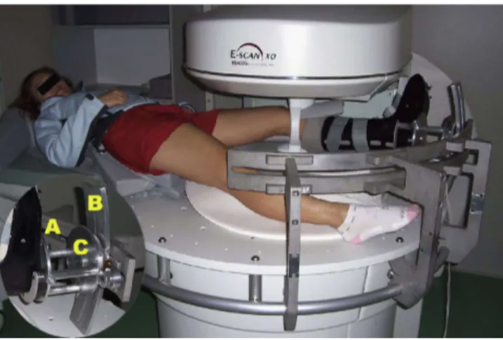
Similarly, to study torsional loading, a torsional loading apparatus can be mounted to an open-MRI patient table [Hemmerich et al. 2009], with open slide rails permitting adjustment of ﬂexion-extension and ab/adduction angles. The subject’s foot is inserted into a plastic boot that is connected to the rotating base, which allows torsional loading of the knee (see ﬁgure 1.4b). However, these methods are limited to static experiments and provide an incomplete picture about human joint behavior [Lavoie et al. 2008]. The knee is motionless when being imaged and thus the result is not dynamic.

The knee under dynamic loading demonstrates a diﬀerent behavior and these methods cannot accurately predict it. Some studies have used dynamic MRI for real-time and in vivo experiments [Seisler and Sheehan 2007] but they note the high cost of the MRI scanners needed. Another study [Williams and Phillips 2005] uses an interventional MRI scanner to study a weight-bearing living knee during squat, but remarks that few such scanners exist worldwide. [Draper et al. 2008] also describes a new real-time MRI to study knee kinematics, including for dynamic dynamic behavior, with a tracking accuracy of up to 2 mm. However, it notes that it cannot be used directly for studying kinematics during walking, but can be used to study just the weight-bearing phases at comparable speeds.

Analyzing human joints in vivo is complicated by the problem of Skin Tissue Artifacts (STA). STA can be defined as the incidence of additional correlated motion of the skin, due to skin and muscle activity, in any body segment motion. STA prevents direct observation of the motion of the tibia and femur bones. A marker fixed to the skin suffers from errors and due to the property of this error being correlated to the actual motion, makes filtering it quite difficult. MRI based studies [Sangeux et al. 2006] show that STAs result in translation errors of up to 22 mm and rotation errors

(19)

6 CHAPTER 1. INTRODUCTION

(a) MRI testbed for studying weight-bearing

knee [McWalter et al. 2010] (b) MRI testbed for torsionally loaded knee. Inset showsloading apparatus for adjusting ﬂexion-extension and ab/adduction rotations (A & B) along with internal-external rotation (C) [Hemmerich et al. 2009]

Figure 1.4: Magnetic Resonance Imaging of the loaded knee of up to 15◦ even without dynamic motion.

One method to overcome the problem of STAs is to attach markers to intra-cortical pins. These pins are drilled into the bone and thus the motion of the markers accurately reflect the motion of the bone [Cappozzo et al. 1996; Reinschmidt et al. 1997] (Fig. 1.5a). Studies have compared the use of intra-cortical pin based markers against skin-based markers [Andersen et al. 2010; Benoit et al. 2006; Leardini et al. 2005; Manal et al. 2002] in determining human bone motion and found that there are significant errors in the calculation of ab/adduction and internal/external rotations when skin based measurements are used. [Fuller et al. 1997] also notes that this STA error lies in the same frequency domain as pin mounted data error, thus making it difficult to filter. However, attaching intra-cortical pins is quite invasive and cannot be replicated on a majority of patients. A subject who once participated in a study involving such methods has been quoted in [Sutherland 2002] as describing his experience as“very painful” and something he would not have agreed to had he understood “what it would be like”.

(a) Intra-cortical pins [Benoit et al. 2006]. (b) Measurement using inertial sensors & skin based optical markers [Cooper et al. 2009].

Figure 1.5: Typical knee gait analysis

(20)

1.2. GAIT ANALYSIS 7 to obtain three dimensional motion data. Fluoroscopic imaging methods have been developed for the kinematic analysis of replaced knee joints [Akbarshahi et al. 2010; Kanekasu et al. 2004; Kessler et al. 2007]. In its simplest form, fluoroscopy based methods include a low dosage X-ray source and a fluorescent screen between which the patient is placed. Flat panel detectors and image intensifiers are coupled to the screen to record the shadows cast by the body. However, as human bones provide a weaker contrast than metallic replacement components, using fluoroscopic imaging for natural knee kinematics leads to reduced accuracy. With these factors in mind, one method used is to measure using fluoroscopy along with CT bone models as described in [Lu et al. 2008; Rahman et al. 2003; Scott and Barney Smith 2006; Yamazaki et al. 2006]. Another method uses orthogonal fluoroscopic images to combine and determine the 6DOF knee kinematics [Li et al. 2004].

X-ray fluoroscopy methods also allow us to study the skin-bone movement by comparing the motion of skin fixed markers with the motion of the bone [Sati et al. 1996]. Such X-ray methods allow for a comparison with classical goniometers [Gogia et al. 1987] to test their reliability. However this method is limited to static and fixed measurements and provides no information of a knee in motion. X-ray based methods have also been developed to allow dynamic recording (at 250 frames/s) as in [Papaioannou et al. 2008], which then uses this data with finite element based methods. Similarly, [You et al. 2001] uses a high-speed bi-plane radiograph along with a CT model to estimate skeletal kinematics. The 2 images from the radiograph are combined with the volumetric CT model to determine the position and orientation of the knee. One must note that exposure to radiation limits the number of tests that can be performed with X-ray based methods.

Diﬃculties in the above mentioned methods lead us to consider optical capture methods. These methods use visible or infrared light to capture the motion of markers [Corazza et al. 2007; Innocenti et al. 2008; Ringer and Lasenby 2004]. The markers can either be attached directly on the skin, or on intra-cortical pins, as mentioned earlier. Marker based methods use predetermined knowledge of the position of the markers relative to the skeleton to estimate the pose of the body segments. They allow us to study deep knee ﬂexion [Zelle et al. 2007], track patellar movement [Lin et al. 2003] and study normal gait [Kadaba et al. 1990; Knoop et al. 2009; Von Porat et al. 2006]. [Ringer and Lasenby 2004] describes a method to automatically estimate the model parameters that describe position of markers relative to the skeleton. Studies such as [Akbarshahi et al. 2010; Camomilla et al. 2009; Cappello et al. 2005; Gao and Zheng 2008] have also used these non-invasive imaging methods to assess the STAs.

Other mocap based methods employ a marker-free system. [Corazza et al. 2007] describes a method to identify joint centers from marker-free data. Figure 1.1 provides an example for the method described in the paper. [Courtney and de Paor 2010] presents a single camera system to automatically record and analyze gait data without markers. The automated system compares well with manual approximations of knee-rotations from the video, but cannot guarantee robustness and accuracy as it lacks 3D position information. [Krosshaug and Bahr 2005] also presents a method that attempts to reconstruct motion patterns from video sequences. It uses a skeletal model to match with the images from the video, and reports favorable results when compared with a skin-marker based system for the ﬂexion angles. However, ab/adduction angle estimates at the hip are shifted while internal-external angles show much higher errors.

A widely used approach is to attach inertial sensors to the patient limbs [Cooper et al. 2009; Favre et al. 2009, 2008; Kawano et al. 2007; Musić et al. 2008; Picerno et al. 2008; Yuan and Chen 2012] (Fig. 1.5b). Inertial sensors readily provide orientation information which allows easy calculation of body pose. Accelerometer orientation and error compensation methods have been proposed by [Latt et al. 2009]. These studies suggest that inertial sensors provide a relatively inexpensive way to observe knee motion.

Accelerometers enable easy identiﬁcation of gait patterns [Torrealba et al. 2007], study center-of-mass displacements [Floor-Westerdijk et al. 2012] and assess energy intensity [Kurihara et al. 2012]. Their small size and mobility enable experiments to be performed outside a laboratory setting. However, accelerometers are prone to drift errors, and over time the velocity and orientation values

(21)

8 CHAPTER 1. INTRODUCTION estimated are unusable. Modern inertial sensors generally include a magnetic sensor, a gyroscope and a 3 axis accelerometer (MARGs). The small size allow it to be packaged as one unit, and data fusion algorithms based on Extended Kalman Filters (or Particle Filters) allow drift-free estimation of the orientations [LaViola 2003; Marins et al. 2001; Sabatini 2006]. However, these still fail to provide us with linear relative position data. A comparison of inertial motion capture systems with optical motion capture can be found in [Cloete and Scheﬀer 2008].

Magnetic sensors can be used along with accelerometers to provide a more robust solution. An applied magnetic ﬁeld with electromagnetic sensors can be used to correct estimates from accelerom-eters [Schepers et al. 2009]. This allows us to limit the maximum error in the estimates. Wearable magnetic sensors can also be coupled with accelerometers as described in [Picerno et al. 2008]. By attaching an exoskeleton to subject leg with an electromagnetic sensor, the position and orientation of body can be tracked, accurate up to ±2.3◦ [Li et al. 2005]. [Amis et al. 2008; Nagamune et al.

2008] describe systems using magnetic sensors for identifying knee joint motion. They also note, however, the isolation from magnetic disturbances that is needed for the study.

Optical markers and accelerometers may not always be attached directly at the skin. In such a case, the the optical marker set is attached using certain configurations, which can affect measure-ment accuracy. The efficiency of various attachmeasure-ment systems has been investigated by [Südhoff et al. 2007] and it describes how three different systems compare with respect to STA. [Amis et al. 2008] also describes a splint-brace attachment for its magnetic sensors.

Another method for knee kinematics is to use ultrasound measurements. [Janvier et al. 2007] describes a ultrasound scanner that aids in 3D reconstruction of limbs. Ultrasound can also be used to study inter-knee distances during walking [Lai et al. 2009]. Plantar pressure also allows additional insight into gait analysis and is frequently employed along with optical motion capture [Miller 2010], or with inertial sensors [Senanayake and Senanayake 2009]

Many studies also choose to model the kinetics of the knee. The muscle and joint contact forces along with kinematic data would assist in diagnosing disorders. In case of patients with replaced knees, studies have utilized instrumented knee implants to measure muscle and contact forces [Lin et al. 2010]. These allows development of better musculoskeletal models. Other studies have used physics-based models to constrain human pose and motion estimation [Brubaker and Fleet 2008]. This model takes into account a dynamic model with joint torques to model muscle forces to improve the accuracy of human pose tracking for walking motions.

Under suitable assumptions, and for specific motions, the three-dimensional motion at the knee joint can be approximated as a spatial single degree of freedom motion. Under such circumstances, the knee can be modeled as a parallel mechanism (described in Section 1.3.2), and we can use these models to analyze the joint motion and develop replacement knees [Di Gregorio and Parenti-Castelli 2006; Ottoboni et al. 2007; Castelli et al. 2004; Saglia et al. 2009; Sancisi and Parenti-Castelli 2010; Wilson and O’Connor 1997]. [Wilson et al. 1998] develops this notion from [Wilson and O’Connor 1997] to predict internal rotation during passive knee flexiion using the mechanism-based approach. [Feikes et al. 2003] proposes a method that improves upon these ideas by using a constraint-based approach instead of a mechanism-based approach to describe the knee flexion as a one degree of freedom motion. The one dof criteria can also be used to model the knee as a four bar mechanism as described by [De Groote et al. 2006] which uses 3D optical measurements over time to estimate the parameters of this model.

This leads us to robots and mechanisms used for gait analysis. Recent studies have experimented with using robotized rehabilitation devices for gait analysis and rehabilitation studies. We discuss these devices in the following section.

1.3 Robots

While notions of automata and mechanical devices exist in the mythologies of many ancient cultures, the word “Robot” (to signify mechanical slaves) was coined in 1920 from the Czech word

(22)

1.3. ROBOTS 9 “robota”, which translates to corvée or serf labor. In an informal sense, the term robot can be used to designate any machine that is used to perform certain tasks automatically or with guidance. Typically, robots are used for manipulating objects for various tasks. In such settings, a robot is a mechanical system that allows the control several degrees of freedom of a rigid body (called end-eﬀector) [Merlet 2010]. The formal deﬁnition used by the European Robotics Research Network, contained in Interna-tional Standard ISO 8373, is that a robot is an ‘automatically controlled, reprogrammable multipurpose manipulator programmable in three or more axes’ [EURON].

In the current sense, robots are generally used as manipulators, where accuracy and repeatability are necessary conditions. Robots (henceforth referred to by the terms robots, manipulators or robotic manipulators interchangeably in this text) can be broadly classiﬁed, based on their architecture, as either serial robots or parallel robots.

1.3.1 Serial Robots

Deﬁnition A serial robot is made up of a succession of rigid bodies from the base to the end-eﬀector, each of them being linked to its predecessor and its successor by one-degree-of-freedom joint.

Figure 1.6: A typical serial robot (SCARA)

Figure 1.6 illustrates a typical serial robot. Serial robots are typically characterized by their low load capacity/robot mass ratio, poor absolute accuracy but ease of design and subsequent kinematic analysis make it the most commonly used architecture.

1.3.2 Parallel Robots

Definition A parallel robot is made up of an end-effector with n degrees of freedom, and of a fixed base, linked together by at least two independent kinematics chains. Actuation takes place through n simple actuators. [Merlet 2010]

While parallel robots are not in as widespread use as serial robots they possess features as a high load capacity/robot mass ratio, minimal number of actuators, high stiffness and high accuracy. Hence they find applications in diverse fields and are used, for example, as flight simulators, tire test rigs, pick and place robots (the Delta robot), active heads of endoscopes, surgical operations, positioning devices, and gaming joysticks.

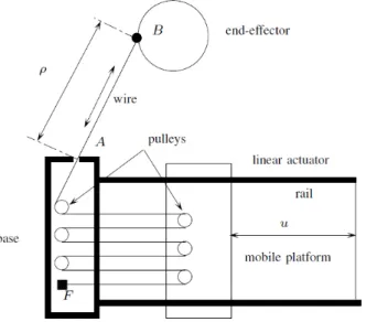
An interesting type of parallel robots are the cable driven parallel robots. In these robots, the end-effector and the base are linked by cables whose lengths are controlled either via rotary actuators (by coiling the cable around a drum) or linear actuators. These robots have the added advantage of being extremely light-weight and modular. A necessary constraint imposed on these robots is that the cables must under tension for effective control of the end-effector.

(23)

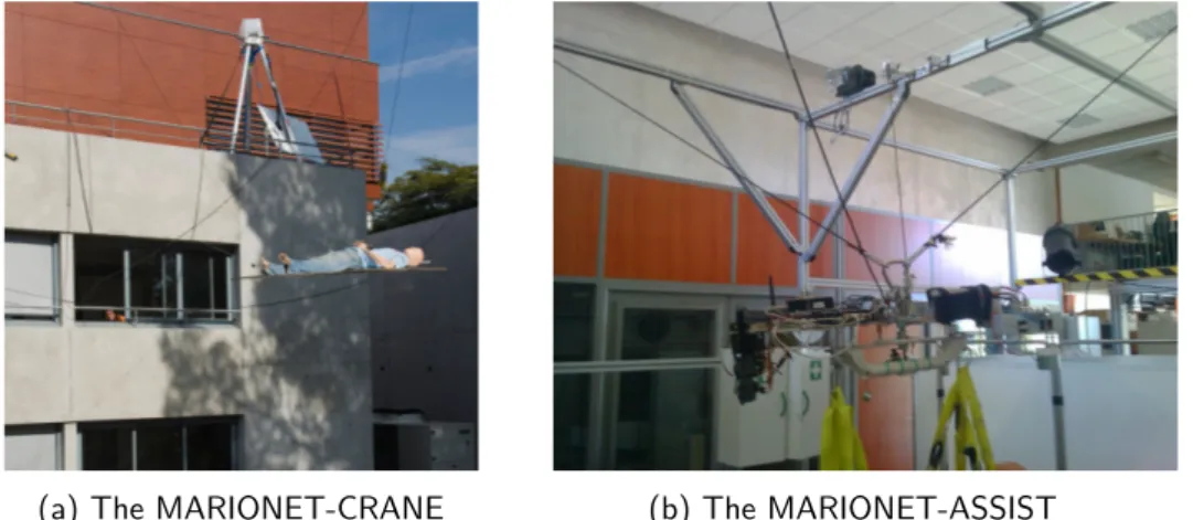
10 CHAPTER 1. INTRODUCTION The COPRIN team at INRIA has developed some prototypes for various applications. The MARIONET-REHAB robot [Merlet 2008] was originally developed as a ultra high-speed parallel manipulator. A detailed description of this robot is provided later on in this thesis. A very large scale version, MARIONET-CRANE (pictured in 1.7a), was developed as a portable, fully autonomous, res-cue crane, with a lifting capacity of over 2 ton. Another version, the MARIONET-ASSIST (pictured in ﬁgure 1.7b), is under development to be used as a home-assistance device.

(a) The MARIONET-CRANE (b) The MARIONET-ASSIST

Figure 1.7: Cable driven parallel robots at INRIA

1.3.3 Robotized Rehabilitation

Robots are used to manipulate the pose of the end-effector accurately. This feature comes in handy in applications such as robots used for diagnostic purposes, an example being a 6DOF artic-ulated arm used to grasp a ultrasound scanner [Janvier et al. 2007]. This system can be trained to accurately scan the lower limb for stenoses and an accurate 3D reconstruction thus created allows for increased diagnosis confidence. However, by designing robots to be back-drivable, we can use the accuracy afforded by them to use the robots as measurement devices. This is the primary idea behind coordinate measurement machines (CMMs) (see figure 1.8). Since actuator displacements

Figure 1.8: A serial backdrivable robot used as a CMM. The Romer portable CMM

are known, the problem of finding pose of the end-effector reduces to a forward kinematics problem. This idea can be extended by designing a manipulator whose end-effector attaches to the human body segment and thus tracks the motion of the body segment. Actuating the manipulator joints allows exerting forces on the body segments to manipulate them into desired poses, which forms the

(24)

1.3. ROBOTS 11 basis of physical therapy. Thus robotic devices that are used to assist the disabled, and those that are used for physical therapy are termed asrobotized rehabilitation devices.

Rehabilitation robots automate the repetitive nature of rehabilitation exercises, allow for the provision of signiﬁcant forces necessary for assistance, and also collect data accurately. This allows for developing an adaptable system that can utilize the expertise of the physiotherapist along with a history of patient progress to develop optimal programs. A historical note on the progress in rehabilitation robots can be found in [Hillman].

Initial applications of robots to rehabilitation focused on adapting pre-existing industrial designs for rehabilitative use. The MIT-MANUS, a 5DOF SCARA mechanism, was developed in 1991 [Hogan et al. 1992] and used for the rehabilitation of shoulder and elbow of stroke patients. It continues to be used giving successful results, with additional extensions being developed [Krebs et al. 2004].

Serial manipulators provide a natural starting point towards developing exoskeletons, or wearable robots. ARMin (figure 1.9) is a serial robotic manipulator with seven actuated degrees of freedom, used as an exoskeleton for the arm. It has been used for stroke patients with promising results [Nef et al. 2009]. Another such exoskeleton based system is the Lokomat gait training (figure 1.10), which also available commercially. It is a robot-assisted modality used for ambulation therapy. While suspended above a treadmill in a secure and stabilizing harness, the robotic legs are fitted to the client’s legs and adjusted to facilitate a fluid, natural walking pattern [LokoMat].

Figure 1.9: The ARMin exoskeleton

for arm rehabilitation [Nef et al. 2009] Figure 1.10: The Lokomat gait training system [LokoMat] Many exoskeleton based devices suffer from the disadvantage of an “always-active” mode. The subject is thus forced to only follow the motion that is performed by manipulator. Researchers at the University of Delaware have overcome these by developing an “assist-as-needed” exoskeleton [Banala et al. 2007] . The ALEX (pictured in figure 1.11) is designed to use a force-field controller to provide zero impedance for desired gait and a high impedance when the gait deviates. Ekso Bionics has developed exoskeletons that allow a wheelchair bound person to stand up and walk. The “Ekso” is a ready-to-wear, battery-powered, bionic device designed for people with lower extremity weakness, paralysis caused by neurological diseases or with injury [Ekso]. This device is a primarily a walking aid, instead of a rehabilitation device (figure 1.12).

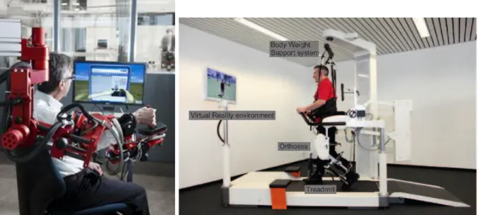
EPFL has developed several rehabilitation robots, including a commercialized product - the Mo-tionMaker [Metrailler et al. 2006] - for knee orthosis. The MoMo-tionMaker also uses a exoskeleton, but has the legs in an unloaded conﬁguration by having the patient situated horizontally. The system has been designed to mimic natural exercises for the knee. Their other rehabilitation device is a vertical gait trainer - the WalkTrainer [Bouri et al. 2006]. Like the exoskeleton based systems, the

(25)

Walk-12 CHAPTER 1. INTRODUCTION

Figure 1.11: The Active Leg EXoskeleton [Banala et al.

2007] Figure 1.12: The Ekso [Ekso]

Trainer (ﬁgure 1.13a) includes elements that are attached to the hip, thigh and shank, and which provide precomputed trajectories to the lower limb. The advantage of this system is that it is not restricted to treadmill scenarios and can provide for natural overground walking. Primarily developed for gait retraining, this system can also be used as a measurement and diagnostic tool.

(a) The WalkTrainer [Bouri et al.

2006] (b) The Lambda [Bouri et al. 2009]

Figure 1.13: Rehabilitation robots at EPFL

One of the major issues with such exoskeleton based systems is the size and energy consumption. As exoskeletons are powered and fitted onto the human limbs, they need actuators positioned at specific points, which add to the bulk. This also calls for a need for efficient power storage that are also light. The safety features, which cannot be ignored, also add to the complexity of the system, as can be seen in the figures provided here (figures 1.10,1.11, 1.12, 1.13a). The rigid designs reduce modularity, while the need for specialized designs adds to their costs.

(26)

1.3. ROBOTS 13 as rehabilitation robots. Their high accuracy allows for safer designs, and high stiffness enables more stable platforms. The limited workspace of certain configurations is not a hindrance as most of the degrees of freedom of human joints have limited range. Parallel robots find an application in ankle rehabilitation robots. The Rutgers Ankle (figure 1.14a) is a Gough platform where the end-effector is fixed to the human foot [Girone et al. 2001]. Another ankle rehabilitation (figure 1.14a) treats the human ankle as a part of the robot kinematic constraints. The Robotic Gait Trainer [Bharadwaj and Sugar 2006] also uses the ankle joint as a part of the design and uses spring over muscle actuators as actuated links.

(a) The Rutgers Ankle [Girone et al. 2001] (b) CAD model - ankle rehabilitation robot [Tsoi et al.2009]

Figure 1.14: Ankle rehabilitation robots

The Lambda (figure 1.13b), at EPFL, uses a parallel robot architecture for rehabilitation and fitness [Bouri et al. 2009]. While this system avoids dependence on anatomical features, its design necessitates additional supports to prevent lateral motions of the leg at the hip joint. Researchers at Laboratory of Robotics and Mechatronics (LARM) at the University of Cassino have developed cable-driven parallel measuring system, CaTraSys. Originally developed for measuring robot kinematic performance, this system has been adapted for gait analysis [Ottaviano et al. 2009]. Cables are attached to the human leg at the shank and the shank is treated as an end-effector of the resultant parallel mechanism. The wire lengths are measured and are used to predict the pose of the shank.

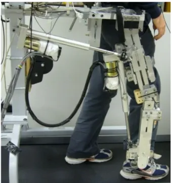
Cable-driven robots have also been developed for neurorehabilitation [Rosati et al. 2007]. The NeReBot, shown in Fig. 1.15, is a three degree-of-freedom wire robot for upper-limb rehabilitation. The advantage of this robot is that it is mounted on a movable frame, potentially allowing its use in domestic rehabilitation. Similarly cable driven robots have been used for gait rehabilitation [Surdilovic and Bernhardt 2004]. Fig 1.16 shows this robot being used. As can be seen, the aim of this robot is to provide support while the patient undergoes walking trials. The robot is used for weight bearing, balancing or posture control while the motion of the lower-limbs is left free. Other sensors, like the knee-goniometers, wire force and position sensors, foot gait-phase sensors are used to track patient motion and control the robot system.

Many of these systems described here suﬀer from being intrusive which may not be accepted easily by subjects. This also limits their adaptability as they cannot be installed into patient homes. The architecture of cable-driven parallel robots allows for developing a modular and light systems, capable of high loads, that can be installed for assisting and rehabilitation purposes. The small size of actuators allows us to reduce the intrusiveness of the system. Further, we have fewer instances of injury if the patient collides with the links i.e the wires. Patient safety can also be enhanced by utilizing wires designed to break at set loads. By ensuring back-drivability, the system could also be used for pose measurement and gait analysis (as in the CaTraSys).

(27)

14 CHAPTER 1. INTRODUCTION

Figure 1.15: The NeReBot [Rosati et al.

2007] Figure 1.16: The String-Man robot configuration[Surdilovic and Bernhardt 2004] Additionally, a cable-driven robot is inherently modular. By using pulleys, the effective base points of the robots are easily changed. Further, designing the cables to be not constrained to have fixed end-effector, and to have the attachment points to be easily changed is a relatively easy task. A cable-driven parallel robot can thus easily adapted based on patient physiological needs, patient anatomy and also according to rehabilitation aims.

Such a system, thus, would serve multiple objectives of physical therapy by allowing: – Diagnostic evaluation of gait patterns

– Detection of anomalies or abnormal motions

– Rehabilitation exercises, where the robot exerts forces to train subject into correct and safe gait patterns

We have developed such a robotic system that includes the cable-driven robot, the MARIONET-REHAB, that forms the focus of this thesis.

1.4 MARIONET-REHAB Gait Analysis system

A cable-based parallel robot measurement system allows us to develop a solution that is extremely modular, and requires simple hardware that is easy to set up. The MARIONET-REHAB is such a cable-based robot developed for gait analysis. The architecture of this robot also allows it to be used for other applications, for example, as a very fast pick and place, for window washing etc. This gait analysis system has been developed to treat body segments as the end-eﬀectors of a cable-based parallel robot. The system includes 7 actuated wires of the MARIONET-REHAB along with 7 passive wires, and the system has been developed to allow any number of wires to be utilized.

The wires are attached to flexible, adjustable collars that attach to the body segments. This allows for modularity and easy reconfiguration for testing all patients using the parallel manipulator architecture. The easy modularity also allows connecting the wires to different body segments with multiple collars and treating the system as multiple cable-based parallel robots with a shared base.

(28)

1.5. CONTENTS 15 To augment the performance of the robotic system and aid the analysis, we populate the system ([Bennour et al. 2011; Harshe et al. 2011]) with additional sensors. The collars are also designed to allow additional sensors to be attached, thus enabling additional information for the end-eﬀectors of the robot. Inertial measurement units can be attached to the collars. Multiple attachment points allow optical markers to be securely fastened and an optical motion capture system is used to track these markers. While these are the main sensors used along with the parallel robot, we also have a provision for force sensors to measure contact forces by the muscles on the collars. In-show pressure sensors and IR reﬂective sensors, to measure the pose of the trunk of the patient, can also be added to the system. These three sensor systems are present for future experiments in cases where additional data might be needed.

While this system would also be able to allow rehabilitation exercises, we only discuss the mea-surement and analysis aspect in this work.

1.5 Contents

This manuscript deals with a system for performing Gait Analysis, whose major component is the MARIONET-REHAB robot, used for tracking the motion of the knee-joint.

In Chapter 2, we provide an overview of the method we use for the analysis of the knee-joint. We explain how our choices motivate the need for various hardware elements (speciﬁcally, a sensor collar) used in the system. Finally, we describe the approach to collate sensor data to obtain usable information regarding the knee-joint.

Next, Chapter 3 details the hardware and software setup developed, the sensors used and the construction of the system. This order of describing the system is chosen as it allows the reader to get an overview of the aims we intend to achieve and see how these are addressed by our setup.

With the overall goal speciﬁed and the robotic system described, we then detail, inChapter 4, the methods used to address the issues that arise from our speciﬁc choice of the setup. This includes the problems of calibration of the hardware, the need for in-experimental re-calibration and the problems of pose estimation.

InChapter 5, we describe the analysis of data for a speciﬁc experiment and the various conclusions we can draw for that example. The methods in the preceding chapters describe the general method of using this modular system while this particular chapter describes how we choose certain parameters for an experiment and how that aﬀects the steps in our analysis.

Finally we discuss the implications and contributions of this work. A plan for future direction of research is laid out, and further applications of this robotic system are also discussed.

(29)

(30)

2 Theoretical Approach

Résumé

Nous étudions au sein de ce chapitre les principaux modèles théoriques d’analyse de la marche. Après avoir présenté les études analysant le genou humain, nous indiquons dans quelle mesure leurs conclusions aﬀectent nos décisions de conception pour notre méthode. Le suivi de mouvement du genou humain rend nécessaire la création d’un modèle cinéma-tique biomécanique. Ce modèle l’articulation du genou ainsi que les deux segments du corps connectés par l’articulation.

Dans la section 2.2, nous présentons les diﬀérents modèles ainsi que le modèle ciné-matique biomécanique choisi pour notre analyse. Nous y explicitons les deux référentiels principaux ainsi que les systèmes de coordonnées utilisés pour les analyses de l’articulation -le premier correspondant aux recommandations des conventions de l’ISB (International So-ciety of Biomechanics) et le deuxième étant déﬁni à partir des données des mouvements des articulations et s’appuyant sur la théorie des torseurs.

Une fois les modèles définis, nous développons dans la section 2.3 les notions d’attache-ment des câbles du robot parallèle aux segd’attache-ments du corps, permettant de considérer ces segments comme les organes effecteurs des robots parallèles. Nous expliquons la géométrie et expliquons la construction d’un collier flexible permettant l’attachement des câbles et l’installation de capteurs additionnels.

A partir de l’utilisation des modèles décrits et des colliers flexibles utilisés (les organes effecteurs du robot parallèle), nous pouvons finalement considérer les méthodes de suivi des articulations. Dans la section 2.4, nous expliquons les paramètres à identifier ainsi que les différentes étapes de fusion de données effectuées à partir d’un filtre de Kalman.

2.1 Overview

In this chapter, we discuss the speciﬁcs of the standard studies that focus on knee analysis and outline how their conclusions have aﬀected our decisions in the design and conception of our method. Tracking a human joint necessitates that a biomechanical kinematic model is created. This model represents the joint and the body segments connected by the joint. Section 2.2 deals with the choice of joint model for the knee.

To observe the motion of this model, our parallel robot system is designed to be attached to the human body and treat the body as its end-effector. However, cables cannot be directly attached to the human body and this entails that some type of collar must be strapped. We also intend to add additional sensors to facilitate analysis and also allow easy comparisons with existing solutions. Thus, the next stage of our analysis details the robot end effector - the flexible collar. The construction and geometry are described in Section 2.3.

Finally, once we have the model of the joint, and the robot end-eﬀector, we focus on steps taken to track the joint. Data from the sensors allow us to estimate the pose of the collar, and thus the body segments. This is described in Section 2.4. This chapter gives a top-down view of the approach we use.

(31)

18 CHAPTER 2. THEORETICAL APPROACH

2.2 Biomechanical modeling

2.2.1 Anatomical & Technical Frames

Observing the motion of human joints involves observing the body segments linked by the joints. To track the knee joint, we must observe the femur and tibia and deduce the joint parameters from the motion data. We do this by attaching coordinate systems to the reference frames ﬁxed to the tibia and femur and observe the relative motion between the two frames. These frames, based on anatomical features and landmarks, can be called Anatomical Frames.

An image-based computational method [Chao et al. 2009] allows for creating three dimensional models to which we can accurately assign coordinate systems using landmarks. However, such meth-ods are diﬃcult to implement in a clinical setting for regular diagnostic purposes. Thus we are tasked with using sensor data and their common local frame, called as the Technical Frame [Cappozzo 2009]. A rigid transformation between the Anatomical and Technical Frames can be obtained from some anatomical calibration methods.

We first describe the classical joint coordinate system that is used for the knee joint, followed by a description of the functional axes based system actually used here.The classical joint coordi-nate system is a type of Anatomical Frame defined using anatomical features, while the functional coordinate system uses Technical Frames to define an anatomical frame.

2.2.2 Classical Joint Coordinate System

A mathematical model of the body segments can be created by setting up the joint coordinate system using the recommendations of the International Society of Biomechanics [Wu and Cavanagh 1995], based on the work by E. S. Grood [Grood and Suntay 1983]. This system possesses the advantage of deﬁning rotations that are sequence independent. They are also easy to interpret clinically.

Referring to Fig. 2.1, the sagittal planefor a body-segment is defined as the plane normal to the axisZin the figure. In case of normal walk, this is the plane in which the body stays approximately, and which includes the vector defining the direction of motion. In this example figure, YX defines the plane, while X is the direction of motion. The sagittal planes for femur and tibia will thus be the planes parallel to this, passing through the center of the respective body segments. The front direction in this plane is referred to as the anterior direction, and the back as the posterior.

The body segment features are further identified by their respective directions from the center. Amedian plane is the plane parallel to the sagittal plane but passes through the center of the body, and divides it into the right and left halves. Features on body segments which are closer to the median plane are identified as “medial”, while those farther away are identified as “lateral”. Thus, on the right half of the body, the lateral direction is given by the vector normal to the median plane, pointing to the right, as given by axis Z (or axes Z1, Z2, Z3 etc) in Fig. 2.1. For body segments on

the left half, this is the medial direction.

Finally, the transverse plane is normal to the sagittal and median plane, and divides the body into the upper and lower halves. The plane allows us to deﬁne the proximal direction as that vector pointing towards the transverse plane, while the distal direction as that pointing away. In Fig 2.1, the axes Y2 and Y3 (i.e pointing upward) refer to the proximal directions, while Y7 (pointing upwards,

but axis ﬁxed to upper body) deﬁnes the distal direction.

We describe the coordinate system for each bone first, and follow it by defining the joint reference axes. The figure 2.2 shows the coordinate system and we provide the definitions here.

Femoral coordinate system

(32)

2.2. BIOMECHANICAL MODELING 19

Figure 2.1: The ISB recommendations for coordinate systems for the human body segments [Wu and Cavanagh 1995]

(33)

Yp The body-ﬁxed axis given by the proximal-distal direction. Proximal direction is considered posi-tive.

Xp Axis in femoral sagittal plane (along anterior-posterior direction), positive direction directed anteriorly.

Zp As deﬁned by right-hand rule. Tibial coordinate system

Origin located at the center of tibial condyles.

Yd The body-ﬁxed axis given by the proximal-distal direction. Proximal direction is considered posi-tive.

Xd Axis, along anterior-posterior direction, directed anteriorly.

Zd As deﬁned by right-hand rule. Joint coordinate system

Yj Along Yd, i.e the tibial axis. Rotations about this axis are the internal/external rotations.

Zj Along Zp. Rotations about this axis are the ﬂexion/extension rotations.

Xj This is a ﬂoating axis, the common perpendicular to Yj and Zj. The positive direction is as deﬁned by the right hand rule. Rotations about this axis are the ab/adduction rotations.

2.2.3 Functional Coordinate System (FCS) - Independence from Anatomical Land-marks

A cursory glance at the ISB recommendations in the section 2.2.2 tells us that the system is highly dependent on the location of anatomical landmarks. Studies show [Marin et al. 2003] that joint angles are not reproducible if they are calculated using coordinate systems set up with anatomical landmarks. In fact, locations of landmarks themselves are subject to errors, as reported in [Croce et al. 1999] where inter-examiner landmark position errors were up to 25 mm. While flexion/extension angle calculations are not dramatically affected, this leads to crosstalk effects and subsequent overestimation of ab/adduction and internal/external angles.

A functional approach deﬁnes a coordinate system using active motion data and is free from measurements of anatomical landmarks.

Instantaneous Helical Axes

One of the fundamental results used in Screw Theory is that any pose change of a rigid body can be eﬀected by a single rotation about an axis, followed by a displacement along the axis [Ball 1900]. This instantaneous axis (or helical axis - HA) for the motion of the femur with respect to the tibia can be obtained without the need for anatomical landmarks. Thus, knee joint motion can be interpreted in terms of the HA [Wolf and Degani 2006], by observing the motion of the HA and then determining the rotation of the femur with respect to the tibia, about the HA.

LetBdenote the 3×3 orthonormal matrix that describes the orientation of the femur with respect

to a global ﬁxed frame. LetMdenote the corresponding matrix for the tibia. Then the relative motion between the two, at time stepi in a sequence of motion, is given by the rotation matrix Ji as,

Ji= BTiMi (2.1)

The instantaneous axis is the axis of rotation η, corresponding to the rotation matrix Ji, which also

(34)

2.3. BIOMEDICAL ROBOT ATTACHMENT 21 Functional Alignment

However, the above described approach is very difficult to interpret clinically. For example, the helical axis in a motion involving flexion will not correspond to that in internal/external rotations. These axes also may not correspond to anatomical features and make it difficult for a clinician to interpret the results. Thus we develop a Functional Coordinate System - an alignment that uses helical axes to define a clinically interpretable and anatomical landmark independent coordinate system.

The methods are described by [Gamage and Lasenby 2002; Mannel et al. 2004; Marin et al. 2003; Rivest 2005], but assume that data are represented in a coordinate system fixed to one of the body segments. These and other methods, surveyed in [Ehrig et al. 2007], provide a framework to define an anatomically interpretable functional coordinate system. The axis identification is done using data obtained from a reproducible motion.

A full squat is one such reproducible motion. It loads the knees equally and the entire range of flexion can be covered. The motion is broken down into finite sequences of motion, and the axes obtained from each step can be used to define an average axis with respect to the individual body segments [Mannel et al. 2004].

The Functional Alignment approach that we intend to use bases its ideas on the above mentioned methods and refines it. The method is defined in [Ball and Greiner 2012] and we provide a brief overview here. The method uses Eq.(2.1)as a starting point to derive a spatial average of the set of rotation matrices Ji in order to get the single best-fit Axis of Rotation (AoR). The goal is to derive

joint-speciﬁc reference framesMA andBA that re-interpretJaround a movement-determined AoR.

We calculate ‘functionally aligned’ rotation matricesFm:

Fm[i] = BTAJ[i]MA (2.2)

and decompose these matrices to Cardan angles.

The Cardan angle representation expresses the orientation using rotations about three indepen-dent axes. This is particularly convenient as it allows us to align the axes with the anatomical features [Chao 1980]. The orientation could be expressed as ﬂexion/extension, ab/adduction and internal/external rotation of the knee (or any joint). These angles are clinically understood and provide an easy reference to the clinician over the rotation matrices obtained from the Functional Alignment approach. A Cardan angle representation would thus facilitate analysis and diagnosis for a physiotherapist.

Thus, our task now is to obtain the body-segment pose matrices B and M for a sequence of motion to be analyzed, using the measurements provided by a set of sensors.

2.3 Biomedical Robot Attachment

2.3.1 Collars

Our aim is to obtain a set of transformation matrices to describe the pose of the thigh (femur) and the shank (tibia). For this purpose, we use a number of skin-based markers placed on the thigh and the shank. We also attach cable to the body segments. However, as brieﬂy noted earlier, the cables cannot be attached directly to the body. Thus, we must use some collars that strap on the body segments and allow the cables of the parallel robot to be attached.

To ensure that markers on the same body segment are fixed rigidly with respect to each other, we attach them too via these collars. These collars thus act as the end effector for the parallel robot, and hold the skin based markers and sensors. As each patient’s anatomical features vary, a rigid collar will be highly impractical and cost-ineffective. Thus, the collars must be adjustable.

In our setup, we propose to use two collars attached to the tibial shank (figure 2.3a), and one on the thigh (figure 2.3b). These adjustable collars are a series of aluminium plates connected by one-degree-of-freedom hinges, with each plate fitted with a pressure sensor. One link in this serial kinematic chain is a flexible, elastic strap that accounts for the variations in the patient’s

(35)

(a) (b)

(c)

Figure 2.3: Collars used in the experiment - (a) Fixed to the tibia (b) ﬁxed to the thigh (c) a collar when extended

characteristics. The hinges allow the collar shape to be changed to fit the patient limb as closely as possible, while the elastic strap permits the collar to be held firmly against the skin (figure 2.3c).

One advantage of this collar is that it reduces overall effect of STA. As sensors are mounted on this collar, local variations in the skin surface position do not affect sensor position. While STA will not be completely eliminated, it will affect the entire collar and thus affect all sensors. Thus, any individual sensor noise can be filtered out. As the plates comprising the collars are fitted with pressure sensors, they allow us to estimate muscle contractions and motions. Although not used in this thesis, the muscle contraction measurements from the pressure sensors would provide us information regarding local STA and may possibly aid in correcting their effects.

The collars are used to hold accelerometer systems (MARG sensors), optical markers, force sensors and include attachment points to connect the passive and active wire systems. The collars are attached to the thigh and tibia, close to anatomical landmarks. We note that variations in patient anatomy results in changes in collar location and reinforces the need for the functional coordinate system described earlier.

The construction of the collar also allows for attaching variable length resistive wires between the collars on the tibia and the thigh.

2.3.2 Construction & Geometry

The collar used to fix sensors consists of styrene plates connected by hinge joints. These hinge joints can be fixed at a constant angle to function as a rigid joint. The plates can be unscrewed from the hinges and quickly replaced. The modular design of the collar ensures that the shape and size can be changed quickly. As a result, these collars can be adapted for use not just on different patients, with differing anatomical dimensions, but also for other experiments to measure motion of other joints.

Of the collars currently developed for the tibia, the lower collar, to be attached just above the ankle (see ﬁgure 2.3a) uses 5 plates, while the upper collar, attached just below the knee, uses 6 plates. All plates in the tibial collar except the front plates are rectangular planar plates with 4 screws