Open Archive TOULOUSE Archive Ouverte (OATAO)
OATAO is an open access repository that collects the work of Toulouse researchers and
makes it freely available over the web where possible.
This is an author-deposited version published in :
http://oatao.univ-toulouse.fr/
Eprints ID : 19379
To link to this article :
DOI: 10.1016/j.sigpro.2017.01.005
URL :
http://dx.doi.org/10.1016/j.sigpro.2017.01.005
To cite this version :
Albughdadi, Mohanad Y.S. and Chaari, Lotfi and Tourneret, Jean-Yves and
Forbes, Florence and Ciuciu, Philippe A Bayesian non-parametric hidden
Markov random model for hemodynamic brain parcellation. (2017) Signal
Processing, vol. 135. pp. 132-146. ISSN 0165-1684
Any correspondence concerning this service should be sent to the repository
administrator:
[email protected]
A Bayesian non-parametric hidden Markov random model for
hemodynamic brain parcellation
M. Albughdadi
a,⁎, L. Chaari
a, J.-Y. Tourneret
a, F. Forbes
b, P. Ciuciu
caUniversity of Toulouse, IRIT, INP-ENSEEIHT, France bINRIA, MISTIS, Grenoble University, LJK, Grenoble, France cCEA/NeuroSpin and INRIA Saclay, Parietal, France
Keywords:
FMRI
Hemodynamic parcellation VEM
Dirichlet process mixture model Non-parametric Bayesian HMRF
A B S T R A C T
Deriving a meaningful functional brain parcellation is a very challenging issue in task-related fMRI analysis. The joint parcellation detection estimation model addresses this issue by inferring the parcels from fMRI data. However, it requires a priorifixing the number of parcels through an initial mask for parcellation. Hence, this difficult task generally depends on the subject. The proposed automatic parcellation approach in this paper overcomes this limitation at the subject-level relying on a Dirichlet process mixture model combined with a hidden Markov randomfield to estimate the parcels and their number online. The proposed method adopts a variational expectation maximization strategy for inference. Compared to the model selection procedure in the joint parcellation detection estimation framework, our method appears more efficient in terms of computational time and does not requirefinely tuned initialization. Synthetic data experiments show that our method is able to estimate the right model order and an accurate parcellation. Real data results demonstrate the ability of our method to aggregate parcels with similar hemodynamic behaviour in the right motor and bilateral occipital cortices while its discriminating power is increased compared to its ancestors. Moreover, the obtained HRF estimates are close to the canonical HRF in both cortices.
1. Introduction
Functional magnetic resonance imaging (fMRI) is a non-invasive imaging technique that indirectly measures neural activity from the blood-oxygen-level dependent (BOLD) signal[31]. This signal reflects the variations in the blood oxygenation level induced by oxygen consumption of neural population involved during task performance. Task-related fMRI data analysis generally focuses on two main issues: (i) detecting the activated brain areas in response to a given stimulus, and (ii) estimating the underlying dynamics associated with such an activation through the estimation of the so called hemodynamic response function (HRF).
So far, many approaches have been proposed to characterize the link between stimuli and the induced BOLD signal through the brain, the simplest relying on a general linear model (GLM) where the link between the stimulus onset and the BOLD effect is actually modelled through a convolution between the HRF and a binary stimulus sequence. The GLM has been primarily used for detecting task-related brain activity in a massive univariate manner [22], considering a constant and fixed canonical HRF shape[6]. Then, it has been progressively extended to
account for the HRF variability using more regressors and hence more flexible design matrices[24,23,29]. Nonetheless, due to the increase of regressors the main difficulty that comes up in this context is the decrease of statistical sensitivity in the subsequent tests, making the detection task less reliable. Besides, other approaches that rely on physiologically-informed non-linear models (e.g., the Balloon model) have been pushed forward for recovering hemodynamics but most often they are deployed in brain regions where evoked activity has already been detected[7,23,33,17]. Their computational cost is actually prohi-bitive for whole brain analysis and some identifiability issues (different pairs of state variables and parameters give the same goodness-of-fit) arise because of the presence of noise. The above mentioned approaches mainly address detection of evoked activity and HRF recovery as a two-step procedure whereas both tasks are strongly linked. A precise localization of activations depends on a reliable HRF estimate, while a robust HRF shape is only achievable in brain regions eliciting task-related activity[26,16]. Moreover, most of linear and non-linear models are designed for univariate inference whereas it is known that the BOLD signal is spatially smooth and thus the HRF shapes remain similar over a certain spatial distance[15,25,3].
⁎Corresponding author.
E-mail address:[email protected](M. Albughdadi).
One of the approaches that accounts for this interdependence is the joint detection-estimation (JDE) framework, where both tasks are performed jointly[30,37,13]. To improve robustness in the estimation task and account for spatial correlation of the BOLD signal, a single HRF shape model was assumed for a specific group of voxels, also referred to as a parcel. Within this JDE formalism, two approaches for posterior inference have been developed, the first one relying on computationally intensive stochastic sampling[30,37]and the second one based on the variational expectation maximization (VEM) algo-rithm[13]to achieve numerical convergence at lower cost. However, whatever the numerical algorithm deployed, the JDE formalism requires a prior parcellation of the brain into functionally homoge-neous regions. These parcels should achieve a fair compromise between
homogeneity and reliability[35]. Homogeneity means that the parcels should be small enough to meet the assumption of HRF shape invariance within each parcel, whereas reliability should guarantee that parcels are large enough to ensure reliable HRF estimation and detection performance. This issue has motivated a number of recent developments that try to cope with the identification of relevant brain parcellation of the brain [20,34,28,27,18]. In Lashkari et al. [27], a non-parametric Bayesian approach, relying on a Dirichlet process mixture model, is considered for the activation classes in a multi-subject framework but they assume that the HRF isfixed for a given region of interest. However, among the latter works, none tries to uncover functional regions that appear homogeneous with respect to their hemodynamic profile. To the best of our knowledge, this issue has been rarely addressed in the literature. In Badillo et al. [2] the hemodynamic parcellation has been addressed using random parcella-tion and consensus clustering. A multivariate Gaussian probabilistic modelling has also been used in Fouque et al. [21]to cope with the hemodynamic parcellation issue. A joint parcellation within the JDE framework has been proposed in Chaari et al.[11,9], giving rise to the joint parcellation detection estimation (JPDE) approach. This strategy performs online parcellation during the detection and estimation steps through the selection of hemodynamic territories, i.e., sets of voxels that share the same HRF pattern. Although automated inference of parcellation is performed in the JPDE methodology, the algorithm still requires the manual setting of the number of parcels. In a previous work Albughdadi et al. [1], we have proposed to finely tune this parameter using an off-line model selection strategy. This procedure was based on the computation of the free energy associated with models of increasing complexity, (i.e., with an increasing number of parcels) in the VEM framework. The best model was then selected as the one maximizing the free energy. This technique was however of limited interest since it requires to run the JPDE algorithm for many candidate models, which is quite time-consuming especially when no prior information is available on the approximate number of parcels. Moreover, even if many analysis have to be conducted on the same subject, running the above-mentioned procedure to select the best model cannot be used only once since the best parcellation and estimation of HRF patterns also depend on the data and not only the number of parcels. Even if the number of parcels is right, the final result can be sub-optimal.
This paper proposes a more original technique to perform on-line model selection by adopting a non-parametric Bayesian (NPB) model. A Dirichlet process (DP) prior combined with a hidden Markov random field is specifically used to estimate the number of parcels from the data itself without any prior knowledge on the initial parcellation. Injected within the JPDE formulation, we end up with an algorithm that needs to be run only once for getting an estimate of the number of parcels and the corresponding HRF territories, with their own hemodynamic signature and evoked responses. Compared with other parcellation techniques, the proposed model allows an automatic estimation of the hemodynamic brain parcels and their number which in turn helps to
improve the detection task and localize the brain regions involved in some mental task. Besides, it allows the hard constraints of a single HRF profile over a given parcel to be relaxed and hence leads to more flexibility in brain analyses. Through this paper, we will refer to the proposed model as the NP-JPDE model.
The rest of the paper is organized as follows.Section 2introduces the Dirichlet process that will be used for hemodynamic brain parcellation. The non-parametric Bayesian model is presented in Section 3. The inference strategy adopted for the proposed model is described inSection 4. Experimental validations on synthetic and real fMRI data are presented in Section 5. Finally, discussions and conclusions are drawn inSection 6.
2. Dirichlet process
Dirichlet processes were first proposed in Ferguson [19]) as distributions placed over distributions. A Dirichlet process (DP), denoted by DP G α( , )0 , is characterized by a base distribution G0and a positive scaling parameter α. More precisely, a random distribution G is distributed according to a Dirichlet Process [19] with scaling parameter α and base distribution G0, if for all natural numbers k and for all k-partitions B{ , …,1 Bk}
G B G B G B Dir αG B αG B αG B
( ( ), ( ), …, ( )) ∼1 2 k ( 0( ),1 0( ), …,2 0( ))k (1) where Dir αG B( 0( ),1 αG B0( ), …,2 αG B0( ))k is the Dirichlet distribution with parameter αG B( 0( ), …,1 αG B0( ))k .
A Dirichlet process mixture model (DPMM) uses the DP as a non-parametric prior in a hierarchical Bayesian model. Let us consider a mixture model where ηnis the parameter associated with the n-th data
point xn, ηnis not observed and the DP is used to induce a prior on the
ηn's. If G is a measure generated according to a DP, G is discrete with
probability one. As a consequence, the following hierarchical repre-sentation can be seen as a countable infinite mixture model
x ηn n∼ (p x ηn n), η Gn ∼GG α G{ , 0} ∼DP α G( , 0) (2) where n= 1, …,N. Among the generated parameter values ηn, a
number of them are equal. These unique values are used to partition the generated x1, …,xN into clusters. Thus, the DPMM is a flexible mixture model with a random number of clusters which grows with new observed data. An explicit DP characterization, which will be useful hereafter, is provided in terms of stick-breaking construction [5]. Consider two infinite collections of independent random variables
τi∼Be(1, ), where Beα (1, ) is a beta distribution with parameters 1α and α, and ηi* ∼G0, for i= 1, 2, …. With τ= , , …τ τ1 2 , the stick-break-ing representation of G is
∏
∑
τ τ πi( ) =τi (1 − ) andτ G= π( )δ . j i j i i η =1 −1 =1 ∞ * i (3) It is clear that G is a discrete distribution whose mixing proportionsτ
πi( ) are given by successively breaking a unit length stick into an infinite number of pieces. The size of each successive piece is propor-tional to the rest of the stick and is given by an independent draw from a beta distribution Be(1, ). Let zα nbe the cluster assignment variable
of the n-th data point. The hierarchical model of a Dirichlet process mixture model can be represented as follows
(i) τ αi ∼Be(1, ),α i= 1, 2, … (ii) η Gi* 0∼G0, i= 1, 2, … (iii) for the n-th data point
(a) znτis distributed according to a multinomial distribution, i.e.,
τ τ
zn ∼Mult π( ( ))with τ= , , …τ τ1 2 (b) x zn n∼ (p x ηn z*)n
3. Non-parametric Bayesian joint parcellation detection estimation model
3.1. Notation
In this paper, a vector is by convention a column vector. The transpose is denoted byt. Matrices and vectors are denoted with bold
capital and lower-case letters (e.g., X and z). We use letters j m, as indexes that run over voxels and experimental conditions, respectively.
3.2. Observation model
The proposed NP-JPDE model considers the observation model used in the JPDE framework proposed in Chaari et al. [11,9]. The JPDE model is the extension of the parcel-based JDE model developed in Makni et al.[30,37]to a whole-brain or a large brain area. We start by recasting the NP-JPDE model. Let7be the set of voxels of interest within the brain mask or the mask of the region of interest (ROI) under study. At voxel j, the fMRI time series yj is measured at times
t n N
{ ,n = 1, …, }, where tn=nTR, N being the number of scans and
TR the time of repetition. The number of different stimulus types or experimental conditions is M. The observed dataY= { ∈yj 5 , ∈j 7}
N is linked to the unknown voxel-dependent HRFsH= { , ∈h jj 7}and the unknown response amplitudes A= {am,m= 1, …,M}
via a unique
BOLD signal model. More precisely, the observation model at each voxelj∈7can be expressed as
∑
yj = a X h +Pℓ +b m M j m m j j j =1 (4)where ajm is the amplitude at voxel j for the m-th experimental
condition witham= {a , ∈j 7} j m
. The ajm's are generally referred to as
neural response levels (NRL). Each NRL is assumed to be in one of I groups specified by latent activation class assignment variables
Q= {qm,m= 1, …,M} where ⎧⎨ 7 ⎩ ⎫ ⎬ ⎭ qm= q , ∈j j m and qj ∈ {1, …, }I m
represents the activation class at voxel j for the m-th experimental condition. Two classes are considered here (I=2) where i=0 and i=1 refer to non-activated and activated voxels, respectively. The binary matrix Xm= {xm ,n= 1, …, ,N d= 0, …,D− 1}
n d t− Δ is a known binary matrix of size N×D that provides information on the stimulus occurrences for the m-th experimental condition, whereΔ ≤t TR is the sampling period of the unknown HRFs. The voxel-dependent HRF is denoted as hj∈5
D
. Each hj is associated with an HRF group. However, the NP-JPDE model does not require to a priori set the optimum number of parcels as in the JPDE model where this number is fixed a priori. Similarly to the activation groups, these HRF groups are specified by a set of latent labelsz= { , ∈z jj 7}where zj∈ {1, 2, …} and zj=k means that the voxel j belongs to the k-th HRF group. An
estimation of z corresponds to a partition of the domain into K hemodynamic territories whose connected components define a par-cellation of the brain or of the considered ROI. Following the stick breaking representation of DP, the mixing proportions of these HRF groups are specified by their stick lengths τ= , , …τ τ1 2 . Finally, the rest of the signal is made of the vector Pℓj, which corresponds to low frequency drifts whereP is an N×Omatrix,ℓj∈5
O
is a vector to be estimated andL= { , ∈ℓj j 7}. Regarding the observation noise, the bj's are assumed to be independent, zero-mean Gaussian vectors with precision matrix Γj. The set of all unknown precision matrices is denoted byΓ= { , ∈Γj j 7}.
3.3. Hierarchical Bayesian model
Adopting a Bayesian formulation for the NP-JPDE model, the joint distribution of the variables Y A H Q z, , , , and τ is defined as follows
Y A H Q z τ Y A H A Q Q H z z τ τ p p p p p p p Θ Θ Θ Θ Θ Θ Θ ( , , , , , ; ) = ( | , ; ) ( | ; ) ( ; ) ( | ; ) ( | ; ) ( ; ) (5)
where Θ is the set of all parameters which will be defined later. More details about the right-hand side term of(5)are provided below. (a) Likelihood
An autoregressive (AR) noise model has been adopted to account for serial correlation in fMRI time series akin to Makni et al.[30], Woolrich et al.[39], Chaari et al.[12,11,9]. Following this model, the covariance matrix at voxel #j is denoted as
σ
Γj= j Λj
−2 where Λ
j is a tridiagonal symmetric matrix whose components depend on the AR(1) parameter ρj. Using the notation
θ0= ( , )σj2 ρj1≤ ≤j J and yj =yj −Pℓj−S hj j with Sj= ∑m a X M j m m =1 , the likelihood factorizes over voxels as follows
⎡ ⎣ ⎢ ⎢ ⎤ ⎦ ⎥ ⎥ ⎛ ⎝ ⎜ ⎜ ⎞ ⎠ ⎟ ⎟
∏
Y A H θ y y p σ σ Λ Λ ( | , ; ) ∝ det exp − 2 . j J j j N j j j j 0 =1 2 (6)(b) Neural response levels
The NRLs are assumed to be statistically independent across conditions, i.e.,
∏
A a θ p( ;θ M) = p( ; ) m M m m {1: } =1 (7)where θmgathers the parameters for the m-th condition. A mixture model is then adopted by using the latent allocation variables qjm
to discriminate between non-activated voxels (qj = 0 m
) and acti-vated ones (qj = 1
m
). For the m-th condition, and conditionally to the assignment variables qm
, the NRLs are assumed to be inde-pendent, i.e., 7
∏
a q θ μ v p( m| m; ) = p a q( | ; , ) m j j m j m m m ∈ (8) with p a q( j| = ;i θ ) ∼5(μ ,v ) m j mm mi mi. All the means and variances of the response amplitudes are gathered in the two unknown vectors
μ= {μmi,m= 1, …,M i, = 0, 1} and v= { ,vmi m= 1, …,M, i= 0, 1}, respectively. Note that for non-activating voxels (i=0) we have set
μm0= 0 for all m= 1, …,M. The other parameters are unknown
and will be estimated. (c) Activation classes
As in Vincent et al. [37], the M experimental conditions are assumed to be independent a priori regarding the activation class assignments, i.e., p( ) = ∏Q m p(q ;β) M m m =1 with p(q ;β) m m a Markov randomfield prior, namely a Potts model with a positive interac-tion parameter βmthat controls the spatial regularization. This
parameter is different from one stimulus type to another and will be estimated. The Potts models prior reads
q q p( m;β) =W β( ) exp(β U( )) m m m m −1 (9) whereU(qm) = ∑ I q( =q ) j l j m l m
∼ , W β( )m is a normalizing constant and
I is an indicator function such that I a( = ) = 1 if a=b and 0b
otherwise. The notation j∼l means that the sum ranges over all neighboring voxels. Moreover, the neighboring system is a 6-connexity 3D scheme. This Markov random field prior accounts for the spatial correlation of the activity, which is one of the physiological properties of the fMRI signal[37].
(d) HRF patterns
The voxel-dependent HRF hjis expressed conditionally to the HRF group variable zjfollowing the JPDE model
7
∏
H z h p( | ) = p( | )z j j j ∈ (10)with p( | = ) ∼hjzj k 5( ,hk Σk) where hk denotes the mean HRF pattern of group k# , whileΣk=νIDadjusts the stochastic perturba-tions around hk via the value of the hyperparameter ν. The HRF
pattern is a priori assigned a zero mean Gaussian distribution 5
hk∼ ( ,0 σh2R) to ensure its smoothness, with R= (Δ ) (t4D D2 2)−1, whereD2is the second-orderfinite difference matrix and σh2is a
parameter to be estimated orfixed. Moreover, hk0=hkD tΔ = 0as in Makni et al. [30], Vincent et al.[37], Chaari et al.[12]. Hence,
5
hk∈ D−1. (e) HRF groups
Following the line of DPMM, we address the issue of auto-matically selecting the number of parcels by considering a coun-table infinite number of parcels. This requires the extension of the standard finite state space Potts model to a countable infinite number of states in which we use a DP prior on thezvariable in the JPDE formulation. Our proposal differs from the one in Chatzis and Tsechpenakis[14]in that it is not a meanfield approximation by a set of independent variables but a direct generalization of the Potts model that uses a stick breaking representation. The stick breaking representation is used to allow for the representation of an infinite number of states. For such a generalization, we need to consider the Potts model with an external field defined over
z= { , …, }z1 zJ for all j= 1, …, , zJ j∈ {1, …, }K such that ⎛ ⎝ ⎜ ⎜ ⎞ ⎠ ⎟ ⎟
∑
∑
z α p( ; , ) ∝ expβz α +β I z( = ) ,z j J z z i j i j =1 ∼ j (11) where βzis an interaction parameter andαis a parameter vectorsuch that α= { , …,α1 αK}represents an additional external field parameter where each αkis scalar. Such a Potts model is defined up
to a multiplicative constant depending on α, meaning that the distribution (11) can be also obtained when adding the same constant value to all the αk's. To avoid such an identifiability issue,
it is common to consider additional constraints on the αk's. One
way to make the parameter vectorαunique is to asssume αk= logπk with∑k π = 1
K k
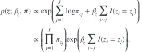
=1 . The Potts model in(11)then rereads ⎛ ⎝ ⎜ ⎜ ⎞ ⎠ ⎟ ⎟ ⎛ ⎝ ⎜ ⎜ ⎞ ⎠ ⎟ ⎟ ⎛ ⎝ ⎜ ⎜ ⎞ ⎠ ⎟ ⎟
∑
∑
∏
∑
z π p β π β I z z π β I z z ( ; , ) ∝ exp log + ( = ) ∝ exp ( = ) . z j J z z i j i j j J z z i j i j =1 ∼ =1 ∼ j j (12) DefineV( ; , ) = ∑z π βz j logπ +β∑ I z( = )z J z z i j i j=1 j ∼ , which is called the energy function, where thefirst and the second sum respectively represents thefirst and the second order potentials. In the finite state space case, such a representation is equivalent, via the Hammersley-Clifford theorem[4], to assume that the distribution in(11)is a Markov randomfield.
Using the stick breaking construction, we can then consider a countable infinite number of probabilities πkthat sum to 1, i.e.,
π
∑k=1 k= 1 ∞
. From this, we can define the same energy function V as before but consider it over an infinite countable set (homogeneous to the set of positive integers),
∑
∑
z π V( ; , ) =βz logπ +β I z( = )z j J z z i j i j =1 j ∼for zj∈ {1, 2, …}. Next, using the Gibbs representation
z z π
p( ) ∝ exp( ( ; , ))V βz , the Hammersley-Clifford theorem still holds if∑ exp( ( ; , )) < ∞z V z π βz . Our choice of π ensures this property.
Indeed, ⎛ ⎝ ⎜ ⎜ ⎞ ⎠ ⎟ ⎟ ⎛ ⎝ ⎜ ⎜ ⎞ ⎠ ⎟ ⎟
∑
∑ ∏
∑
∑ ∏
z π V β π β I z z β J J π β J J exp( ( ; , )) = exp ( = ) < exp( ( − 1)) < exp( ( − 1)) < ∞ z z z z j J z z i j i j z j J z z =1 ∼ =1 j jwhere J J( − 1) is the maximum number of neighbors among J sites. We also used that for all j= 1, …, ,J ∑zπz = ∑k=1πk= 1
∞
j j . It follows
that p( ; , )z π βz, in the infinite state space case, is still a valid probability distribution and is a Markovfield by the Hammersley-Clifford theorem. Note that such a generalization of the Potts model is possible because of the presence of the externalfield parameters πkthat satisfy∑k=1πk= 1
∞ . A Potts model with equal externalfield parameters cannot be as simply extended to an infinite countable state space. For a Potts model with no external field, such an extension is not possible because in the K-state case this Potts model is equivalent to πk= 1/Kfor all k where their sum does not
tend to 1 when K tends to infinity. In the stick breaking setting, we then considerπk( ) =τ τk∏l (1 − )τ k l =1 −1 and ⎛ ⎝ ⎜ ⎜ ⎞ ⎠ ⎟ ⎟ ⎛ ⎝ ⎜ ⎜ ⎞ ⎠ ⎟ ⎟
∏
∑
z τ τ p( ; , ) ∝βz π ( ) exp β I z( = ) .z j J z z i j i j =1 ∼ j (13) Such a construction is valid for any set of parameters τ= { }τk k∞=1 with each τk∈ [0, 1].(f) Stick lengths
Following (13) would leave us with an infinite number of parameters τkto estimate. The Bayesian point of view solves this
problem by assuming that all τk's are i.i.d. variables following the
same Be(1, ) distribution so that the number of parameters toα
estimate is now reduced to a single parameter α. The stick lengths are a priori assigned a beta distribution with parameters 1 and α,
i.e.,
p τ α(k ) ∼Be(1, ) forα k= 1, 2, …. (14) The scaling parameter α may have a significant effect on the growth of the number of parcels. Following Blei et al.[5], a gamma prior is placed over α with parameters s1 and s2, i.e., α∼ gamma(s , s )1 2 where α s, 1and s2will be estimated.
The extension of JPDE model to an infinite number of parcels therefore consists of augmenting the original JPDE formulation with additional variables{ }τk k∞=1and of considering the following hierarchical construc-tion that yields the NP-JPDE model
(i) p τ α(k ) ∼Be(1, ),α k= 1, 2, … (ii) ( * = ( ,Θk hk Σk)G0) ∼G0,k= 1, 2, …whereG0=5(0,σh2R) ⊗δνI (iii) p( | ; ) ∝ ( ∏z τ βz j π ( ))exp( ∑τ β I z( = ))z J z z i j i j =1 j ∼
(iv) hj zj∼ ( | *)phjΘzj, where p( | *) =hjΘk 5( ;h hj k,Σk)is a Gaussian dis-tribution whose parameters h Σk, k are associated with the k-th parcel.1
where Θ= { , , , ,Γ L θa β σz h2, ( )hk1≤ ≤k K, , }ν α . The probabilities τ
p( ) = ∏k=1p τ( )k
∞ and p( | )z τ are defined in steps (i) and (iii), respec-tively.
Fig. 1illustrates the hierarchical model of the NP-JPDE model.
1The other distributions de
fining the model remain the same as in the standard JPDE model. Note that in the extended version above we assume νk=νfor all k to define G0.
4. Variational expectation maximization algorithm
Different inference strategies can be used to estimate the missing variables A H Q z, , , and τ in addition to the parameters Θ from the posterior p( ,A H Q z τ Y, , , ;Θ) associated with(5). Due to the compu-tational complexity of MCMC methods, we here use a VEM algorithm to derive an approximation of the true posterior distribution
A H Q z τ Y p( , , , , ;Θ) of the form
∏
∏
A H Q z τ A H τ p( , , , , ;Θ) =p( )p ( ) p ( )Q p z p( ) ( ). ∼ ∼ ∼ ∼ ∼ ∼ A H j J Q j j J z j τ =1 j =1 j (15)In the variational distribution above, the approximations∏j p∼ ( )Q
J Q j =1 j and∏j p z∼( ) J z j
=1 j are sought in a form that factorizes over voxels (mean
field) to handle intractability due to the spatial neighborhood. Following Blei et al.[5], the infinite state space forzis dealt with by considering a truncation to a number K which consists of assuming that the variational distribution satisfies p k∼zj( ) = 0 for k>K and
τ p( ) = ∏ p τ( ) ∼ ∼ τ k K τ k =1 −1
k . This amounts to setting τk= 1 for k≥K or
p τ( ) = ( )δ τ
∼
τk k 1 k. It is worth noticing that in this case the Dirichlet process is still full and not truncated. Moreover, the truncation level is freely adjusted without being a part of the prior model specification[5].
The VEM approach requiresfive steps associated with five expecta-tions referred to as: VE-H, VE-A, VE-Q, VE-Z andVE − . The resultingτ
E-steps can be written as ⎛ ⎝ ⎜ ⎞ ⎠ ⎟ H H Y A z p p VE− :H ∼H ( ) ∝ exp E [log ( | , , ;Θ ] r p p r ( ) ( −1) ∼ ∼ A( −1) ( −1)r zr (16) ⎛ ⎝ ⎜ ⎞ ⎠ ⎟ A A Y H Q p p VE− :A ∼A ( ) ∝ exp E [log ( | , , ;Θ )] r p p r ( ) ( −1) ∼ ∼ H( ) ( −1)r Qr (17) ⎛ ⎝ ⎜ ⎞ ⎠ ⎟ Q Q Y A p p VE− :Q ∼Q ( ) ∝ exp E [log ( | , ;Θ )] r p r ( ) ( −1) ∼ A( )r (18) ⎛ ⎝ ⎜ ⎞ ⎠ ⎟ τ p τ pτ Y z VE− : ∼z ( ) ∝ exp E [log ( | , ;Θ )] r p r ( ) ( −1) ∼ z( )r (19) ⎛ ⎝ ⎜ ⎞ ⎠ ⎟ z z Y H τ p p VE− :Z ∼z ( ) ∝ exp E [log ( | , , ;Θ )] . r p p r ( ) ( −1) ∼ ∼ H( ) ( )r τr (20)
Compared to the standard JPDE model, the new steps are the VE-Z and
τ
VE− steps which are detailed below. To make the paper self-contained, more details about the other expectation steps are provided inAppendix A.
•
VE−τstep This step is straightforwardly driven from results on variational approximation in the exponential family. Given(3)and for k= 1, …,K− 1, ⎛ ⎝ ⎜ ⎜ ⎡ ⎣ ⎢ ⎤⎦⎥ ⎞ ⎠ ⎟ ⎟∑
τ p τ( ) ∝ ( )expp τ E log ( )π ∼ τ k k j J p p z =1 ∼ ∼ k zj τ⧹{ }k j (21) ⎛ ⎝ ⎜ ⎜ ⎞ ⎠ ⎟ ⎟∑ ∑
∑
p τ p l τ p k τ∝ ( )expk ∼( )log(1 − ) + ∼( )log( ) j J l k K z k j J z k =1 = +1 j =1 j (22) Be γ γ ∝ (k,1, k,2) (23) with
∑
∑ ∑
γk = 1 + p k∼( ) and γ =α+ p l∼( ). j J z k j J l k K z ,1 =1 ,2 =1 = +1 j j (24)•
VE-Z step This step is divided into J VE-Zjsteps. Since we assumep z( ) = 0 ∼
zj j for zj>K, we only need to compute the distributions for
zj≤K, ⎛ ⎝ ⎜ ⎜ ⎡ ⎣ ⎢ ⎤⎦⎥ ⎞ ⎠ ⎟ ⎟
∑
h τp z( ) ∝ exp E [log ( | )] + Ep z log ( ) +π β p z( )
∼ ∼ z j p j j p z z i j z j ∼ ∼ ∼ j Hj τ j i (25) where
∑
τ π τ τE [log ( )] = E [log ] +p k p k E [log(1 − )]. l k p l =1 −1 ∼ ∼ ∼ τ τk τl (26)
The expectations above can be computed using the fact that p∼τkis a beta distribution, i.e., Be γ(k,1,γk,2)defined by(24)
τ Ψ γ Ψ γ γ
E [log( )] =p∼τk k (k,1) − (k,1+ k,2) (27)
τ Ψ γ Ψ γ γ
E [log(1 − )] =p∼τk k (k,2) − (k,1+ k,2) (28) whereΨ(. )is the digamma function defined by
Ψ z d dz Γ z Γ z Γ z ( ) = log ( ) = ′( ) ( ). The termEp∼ [log ( | )]phjzj
Hj is computed as 5 h m h p z Σ Ep∼ [log ( | )] ∝j j ( H; k, k). Hj j (29)
where mHjis the mean of the voxel-dependent HRF obtained in the VE-H step (seeAppendix A(i)).
•
VM step The maximization step in this extended NP-JPDE isdifferent when compared to the one of the JPDE model in Chaari et al.[9]. As a consequence of the added hierarchical terms, it can be rewritten as
Fig. 1. Graphical model describing dependencies between observed and latent variables involved in the NP-JPDE generative model for a given region of interest with J voxels. Observed variables are shaded in grey. J and M refer to the voxel and stimulus levels, respectively.
Y A h L A Q μ v h z h Q β z τ τ p p p p p β p α Θ Γ Σ
= argmax{E [log ( | , ; , )] + E [log ( | ; , )]
+ E [log ( | ; { , } ]
+ E [log ( ; )] + E [log ( ; )] + E [log ( ; )]}.
r pArpHr pArpQr pHrpzr k k k K pQr pzrpτr z pτr Θ ( ) ( ) ( ) ( ) ( ) ( ) ( ) =1: ( ) ( ) ( ) ( ) ∼ ∼ ∼ ∼ ∼ ∼ ∼ ∼ ∼ ∼ (30) The two new maximization steps of the NP-JPDE model when compared to the JPDE one are associated with the parameters α and βz. Maximizing(30)with respect to α leads to
τ αr = argmaxE [log ( ; )]p α α p ( ) ∼ τ( )r (31)
where a gamma prior is placed over the scaling parameter α with parameters( , )s sl l1 2. The gamma distribution is conjugate to the stick lengths and the parametersls1andls2are given by
l l
∑
s =s +K− 1 and s =s − E [log(1 − )].τ k K p k 1 1 2 2 =1 −1 ∼ τk (32)After computing these parameters, we replace α in (24) with its expectationE [ ] =qα ll
s s 1 2.
Maximizing(30)with respect to βzleads to
z τ βz = argmaxE [log ( | ; )].p β r β p p z ( ) ∼ ∼ z z r τr ( ) ( ) (33) This step does not admit an explicit closed-form expression but can be solved numerically using gradient ascent schemes. This solution is computationally expensive. For this reason, the experiments con-sidered hereafter were conducted with afixed value of βzadjusted
using cross validation. 5. Validation
The NP-JPDE model was validated using synthetic and real data experiments via appropriate comparisons to assess its performance.2
These experiments are described in this section.
5.1. Synthetic fMRI time series
First, the proposed non-parametric Bayesian algorithm is compared with the strategy adopted in Albughdadi et al. [1]which consists of selecting the model that provides the highest free energy. In a second step, the performance of the NP-JPDE model is assessed for large grid size and number of parcels in the ROI under study. Thefinal part is dedicated to highlight the difference between the automatic hemody-namic brain parcellation provided by the NP-JPDE model and other parcellation techniques from the literature.
•
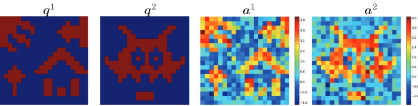
NP-JPDE model validation and comparison with other hemodynamic parcellation algorithms (JPDE model)To validate the NP-JPDE model, three different synthetic experi-ments referred to as Exps 1–3 were conducted. Different parcellation masks were used in each experiment to generate BOLD signal according to(4). Two experimental conditions (M=2) were consid-ered with 30 trials for each of them. The reference activation labels are shown inFig. 2(q1andq2). Using Pyhrf, the NRLs were drawn according to their prior distribution conditionally to the activation labelsQofFig. 2. Given these 20×20 binary labels, the NRLs were simulated as follows, for m= 0, 1:a qj| = 0 ∼5(0, 0.5)
m j m and 5 a qj| = 1 ∼ (3.2, 0.5) m j m
(Fig. 2(a1anda2). The onsets of these trials were randomly generated with a mean inter stimuli interval of 3 s and a variance of 5 s. The fMRI time series yj were then generated according to(4)usingΔ = 0.5t and TR=1 s. As a ground truth for the
parcellation, different HRFs groups were considered, each with
Kω=ω+ 1
parcels where ω∈ {1, …, 3}. The HRFs associated with these groups were selected from the ground truth HRFs( )hk k
K =1
ω
shown in Fig. 3. Reference parcellations for the three experiments are displayed inFig. 4. These reference parcellations were chosen with different cardinalities and overlap with activation areas in order to investigate the robustness of the NP-JPDE model to the total amount of evoked activity in each parcel. Indeed, from a statistical point of view, the estimation of parcels involving a large amount of activated voxels should be more accurate than the estimation of parcels overlapping only a few activated voxels. Importantly, to mimic a real scenario in all experiments, we set the percentage of the activated voxels to be approximately 53% of the total number of voxels (this percentage was calculated by performing a bitwise OR between the reference activation binary labels of the two experimental conditions Fig. 2). Table 1 reports for each experiment the percentage of activated voxels in each parcel of the ground truth. These synthetic fMRI time series were then processed by the JPDE and NP-JPDE models. Results obtained with the two models were compared especially in terms of model selection. When using the original JPDE, three competing models Kω=ω+ 1
where ω∈ {1, …, 3} were run and their corresponding free energy values were computed following the proposed model selection procedure in Albughdadi et al. [1]. As regards the NP-JPDE, it is worth noting that we do not need to specify any specific initialization. Hence, the latter was done ran-domly in contrast to the shown initializations for the original JPDE reported inFig. 4[bottom]. The NP-JPDE model only requires to set the maximum number of parcels K (truncation level) for the varia-tional approximation. This number was set to K=20 for the three experiments, while the Potts parameter βzwasfixed to 1.2 for the
spatial regularity of the parcellation.3The parameter βmfor
activa-tion classes which corresponds to the m-th experimental condiactiva-tion is estimated in the maximization step (as inAppendix A(v)). The prior values over the scaling parameter α of the DPMM were set to
l l
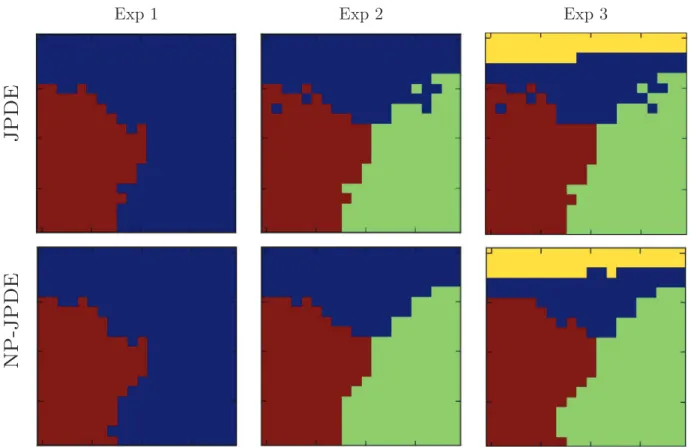
s1= 20,s2= 5to be estimated in the VEM algorithm. The estimated parcellations obtained by the two JPDE versions are shown inFig. 5. Thisfigure shows accurate parcellation estimates from a visual point of view. A comparison with the ground truth allows one to conclude that the proposed NP-JPDE algorithm recovers accurate parcels especially for activated parcels. Quantitative evaluation of the parcel-lation estimates is provided inTable 2 where the error rate with respect to the ground truth is given. First, one can notice the small error probabilities for both models in all experiments. Furthermore, the NP-JPDE outperforms the original JPDE seen in the error reported for experiments 2 and 3. This remark corroborates the better visual performance of the proposed NP-JPDE model. To investigate more deeply the robustness of the parcellation estimation using the NP-JPDE model, the confusion matrix for each of the three experiments was computed and shown inTables 3–5. We observed that the proposed NP-JPDE is highly accurate regarding the parcella-tion estimaparcella-tion step as the overlap between the reference and estimate for each parcel is larger than 95% in all experiments.
In order to further investigate the robustness of the proposed model,Table 6provides the mean square errors (MSEs) for the NRLs and activation labels associated with the JPDE and NP-JPDE models. These results corroborate the fact that the NP-JPDE model ensures precise estimation of the NRLs for both experimental conditions and outperforms the classical JPDE version. The construction of the parcellation for the NP-JPDE model has therefore very little impact on the NRL estimates and the detection task. Next, we investigated the accuracy of the estimation task by looking at the HRF estimates using the NP-JPDE model as reported inFig. 6. A comparison between the reference and estimated HRF shapes shows that the NP-JPDE model is
2These experiments were implemented in Python within the framework offered by the
Pyhrf software[36], see alsohttp://pyhrf.org. 3This value of β
able to recover precise hemodynamics profiles and they are close to the HRF estimates of the original JPDE version (shown in the same figure).
Last, we studied the convergence of the number of parcels over
iterations within the NP-JPDE. To this end, we present inFig. 7the parcellation estimate for Exp 2 along different iterations until con-vergence. Starting with a random initialization, thisfigure shows that after about 7 iterations all the main parcels are well established. Furthermore, for the same experiment,fifty runs of the VEM algorithm using different random initializations were performed and the sub-sequent box plot graph was drawn to investigate the sensitivity of the NP-JPDE model to this setting. Fig. 8shows the evolution of the number of parcels over iterations for thefifty runs. It appears first that
Fig. 2. Reference activation labels and NRLs for the two experimental conditions (grid size=20 × 20).
Fig. 3. Ground truth HRF shapes h k( ,k = 1, …,Kω with ω= {1, …, 3}) used for
generating synthetic fMRI time series.
Fig. 4. Ground truth parcellations used for the 3 experiments and corresponding initialization masks (only used for the original version of the JPDE approach) (grid size=20×20). Table 1
Percentage of activated voxels in each parcel of the ground truth parcellations for the three experiments. The parcels indexes are shown inFig. 4.
# Parcel Exp 1 Exp 2 Exp 3
1 66.7% 22.2% 19.5%
2 33.3% 44.5% 44.5%
3 – 33.3% 33.3%
all the parcels were present after thefirst few iterations. Second, this number decreased through the iterations. Finally, we investigated the computational load. For doing so, we computed the running time for the standard JPDE framework by accumulating all elapsed times required for assessing the free energy associated with each candidate model, as done in Albughdadi et al.[1]. Using a machine with 8 cores, each corresponding to anIntel® Xeon(R) CPU E3-1240 v3 chipset clocking at 3.40 GHz processor and 16 GB of RAM, the four investi-gated models in the classical JPDE framework run in about 35 mins whereas for the NP-JPDE model it takes less than 9 min. Thus, the computational cost of the NP-JPDE model is reduced when compared
Fig. 5. Parcellation estimates for the three experiments using the original JPDE and NP-JPDE (grid size=20×20).
Table 2
Error probabilities on the parcellation estimates using the original JPDE and the NP-JPDE algorithms.
Model Exp 1 Exp 2 Exp 3
NP-JPDE 1.5% 0.25% 1.5%
JPDE 1.5% 2.75% 3.25%
Table 3
Confusion matrix for Exp 1. (NP-JPDE model). RP and EP refer to the reference and the estimated parcellations, respectively.
RP
EP Parcel 1 Parcel 2
Parcel 1 1.0 0.046
Parcel 2 0.0 0.954
Table 4
Confusion matrix for Exp 2. (NP-JPDE model). RP and EP refer to the reference and the estimated parcellations, respectively.
RP
EP Parcel 1 Parcel 2 Parcel 3
Parcel 1 1.0 0.0 0.008
Parcel 2 0.0 1.0 0.0
Parcel 3 0.0 0.0 0.992
Table 5
Confusion matrix for Exp 3. (NP-JPDE model). RP and EP refer to the reference and the estimated parcellations, respectively.
RP
EP Parcel 1 Parcel 2 Parcel 3 Parcel 4
Parcel 1 1.0 0.013 0.0 0.0
Parcel 2 0.00 0.961 0.0 0.0
Parcel 3 0.0 0.0 1.0 0.023
Parcel 4 0.0 0.026 0.0 0.977
Table 6
MSEs of NRL estimates and activation labels for the JPDE and NP-JPDE models.
Exp 1 Exp 2 Exp 3
JPDE NP-JPDE JPDE NP-JPDE JPDE NP-JPDE
NRLs m=1 0.016 0.007 0.017 0.008 0.017 0.008
m=2 0.012 0.006 0.012 0.006 0.012 0.006
Labels m=1 0.003 0.004 0.011 0.003 0.011 0.003
to free energy calculations of many candidate models.
•
Case study: The NP-JPDE model for a large grid size andmore parcels
Exp 4 was conducted using synthetic BOLD fMRI time series for a grid size of 200×200 with 11 parcels. The generated synthetic data was tested using the NP-JPDE model with the same experimental
setup described inSection 5.1. The estimated parcellation using the NP-JPDE model is shown inFig. 9 along with the ground truth parcellation. The error probability of parcellation was 1.6%. As regards the HRF profiles of the estimated parcels, they are shown in Fig. 10along with their ground truths where we can see a good match between the estimates and references. Moreover, it is interesting to note that even the HRFs of parcel 5, 6 and 8, 11 have similar characteristics, the NP-JPDE model is still able to discrimi-nate them. The time to peak (TTP) and full width at half maximum (FWHM) values of the ground truth and estimated HRFs are
Fig. 6. HRF estimates for the three experiments using JPDE and NP-JPDE models.
Fig. 7. Parcellation estimates for Exp 2 using the NP-JPDE model along successive iterations (grid size=20×20).
Fig. 8. Boxplot forfifty different runs of Exp 2 using the NP-JPDE model showing the convergence of the parcellation up to 30 iterations. The convergence is achieved from iteration 16.
Fig. 9. Parcellation estimates obtained using the NP-JPDE model for a synthetic fMRI BOLD time series with 11 parcels (grid size=200×200).
summarized inTable 7. These results confirm that the NP-JPDE model is still reliable for larger number of parcels and grid size.
•
Comparison with other parcellation methodsFinally, we use the synthetic data of Exp 2 to compare the hemodynamic parcellation obtained using the NP-JPDE model with other parcellation approaches as the K-means and Ward's algo-rithms [35,38]. The parcellation results of these algorithms are shown inFig. 11. It is clear that both algorithms are not able to detect the three hemodynamic territories in the ground truth (Fig. 4[middle-top]). Moreover, the estimated parcellations are also affected by the activation labels of the two experimental conditions. This observation confirms that the standard parcellation techniques can be easily influenced by the BOLD signal level in the activated area.
5.2. Real data
Two experiments were conducted on real fMRI data to validate the proposed NP-JPDE model with two regions of interest (ROI) under consideration. Exp 7 and Exp 8 focused on the right motor and bilateral occipital ROIs, respectively. These ROIs are shown inFig. 12and were defined from the statistical results of a standard subject-level GLM analysis of fMRI data. More precisely, Student-t maps associated with the two contrasts of interest, namely (Left Click - Right Click) and (Visual stimuli - Auditory stimuli), were thresholded at
p=0.05, corrected for multiple comparisons according to the FWER
criterion, see Badillo et al.[3], Chaari et al.[10]for details. The fMRI data were collected using a gradient-echo EPI sequence (TE=30 ms/ TR=2.4 s/thickness=3 mm/FOV=192×192 mm2, matrix size: 96×96) at a 3 Tesla during a localizer experiment[32]. Sixty auditory, visual and motor stimuli were involved in the paradigm and defined in ten experimental conditions M( = 10) (see[3,10]for details). During this paradigm, N=128 scans were acquired. For both experiments, we considered the truncation level K=20, the parameter of the HMRF βz
was empirically set to 1.8 and the parameters of the gamma prior for
Fig. 10. HRF estimates obtained using the NP-JPDE model for a synthetic fMRI BOLD time series with 11 parcels (Exp 4).
Table 7
Computed TTP and FWHM for the ground truth and estimated HRFs of the parcels in Exp 4 where the identical values are in bold font.
HRF Ground truth Estimated
TTP FWHM TTP FWHM HRF 1 2.0 5.5 2.0 5.5 HRF 2 5.0 6.0 5.0 6.0 HRF 3 6.0 7.0 6.0 7.0 HRF 4 8.0 8.5 8.0 8.5 HRF 5 4.0 9.0 3.5 9.0 HRF 6 5.0 9.5 5.5 9.5 HRF 7 10.0 7.0 10.0 6.5 HRF 8 11.0 7.5 10.5 7.5 HRF 9 12.0 7.5 11.5 7.5 HRF 10 9.5 7.5 9.5 7.5 HRF 11 11.0 7.0 11.0 7.5
the scaling parameter α were set tols = 201 ,ls = 52 .4
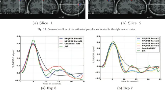
In Exp 5, two parcels were estimated in the right motor cortex. Different slices of the estimated parcellation are shown inFig. 13. The HRF shape estimates are shown inFig. 14(a) along with the canonical HRF and the HRF estimated with the JDE model. These HRF estimates have the same value of the time to peak (TTP) and the full width at half maximum (FWHM): TTP=4.8 s and FWHM=4.2 s. As regards the HRF obtained with JDE, the TTP and FWHM values are 4.8 s and 3.6 s, respectively. We notice that both models recover the same TTP whereas the JDE yields a slightly narrower HRF (lower FWHM). The Euclidean distances between the HRF estimates themselves and the canonical HRF are reported inTable 8indicate that the NP-JPDE model provides closer HRF estimates to the canonical one (average Euclidean distance
of 0.4) compared to the JDE model (average Euclidean distance of 0.43). In this sense, the NP-JPDE model provides more coherent results than the JDE one in terms of closeness of the HRF estimates to the canonical shape in the motor cortex as it has already been shown in the literature [3]. As regards the NRL estimates, the focus of the experiment is on the left and right click visual and auditory experi-mental conditions which are expected to elicit evoked activity in the right motor cortex. Taking the left and right auditory experimental conditions as an example,Fig. 15shows the NRL estimates using the NP-JPDE and JDE models (with respect to the left and right auditory experimental conditions) and the computed contrast (auditory left click-auditory right click). These results confirm the coherence between the NRL estimates obtained with the JDE and NP-JPDE models, especially in terms of maximum activation location and amplitude values.
The NP-JPDE was also run for Exp 6 on the bilateral occipital cortex. Four parcels were detected as shown inFig. 16. The corre-sponding HRF shape estimates for these parcels are shown in Fig. 14(b). These HRF estimates are displayed along with the canonical HRF and the one estimated using the JDE model. The computed TTP for the HRF profiles of parcels 1, 2 and 4 is TTP=5.4 s, while for parcel 3 we have TTP=6.0 s. The FWHM was also computed and is equal to 4.2 s for parcels 1 and 4, and to 4.8 s for parcels 2 and 3. As regards the HRF estimated using the JDE model, we have TTP=5.4 s and FWHM=4.2 s. Moreover, Table 9 reports the computed Euclidean
Fig. 12. Anatomical localization of brain regions. On top, the ROI is located in the right motor cortex and consists of a single connected component. At the bottom, the ROI is located in the primary visual cortex and made up of two connected components, one in each hemisphere.
Fig. 13. Consecutive slices of the estimated parcellation located in the right motor cortex.
Fig. 14. HRF shape estimates using the NP-JPDE and JDE models in the right motor cortex (a) and the bilateral occipital cortex (b) along with the canonical HRF.
Table 8
Euclidean distance between the HRF estimates in the right motor cortex and the canonical HRF. Distance between the individual NP-JPDE HRF estimates are also provided.
HRF 1 HRF 2 JDE
Canonical HRF 0.37 0.43 0.43
HRF 2 0.30 – –
distances between the different HRF estimates and the canonical HRF. It also reports the same distance between the individual NP-JPDE HRF estimates. The reported distances indicate that the NP-JPDE model provides closer HRF estimates to the canonical shape with average Euclidean distance of 0.42. More interestingly, it is clear that the NP-JPDE model is able to discriminate between parcels that have very close HRFs in terms of Euclidean distance, namely those of parcels 1 and 2. Indeed, these two parcels have similar TTPs, but different FWHM values. They are therefore detected as different parcels by the NP-JPDE model.
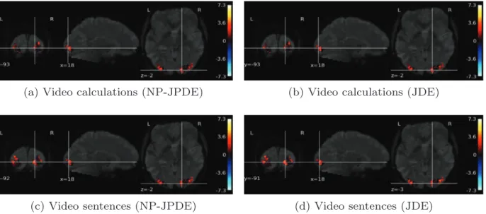
Fig. 17 shows the NRL estimates for some of the experimental conditions which are supposed to induce evoked activity in the bilateral occipital cortex (namely, video calculations and video sentences). The obtained NRL estimates with the NP-JPDE and the JDE are similar in terms of amplitude values and the location of the highest activation. 6. Discussion and conclusion
In this paper, we proposed a new approach to estimate the number of hemodynamic parcels in fMRI data analysis where model selection was formulated as a clustering issue. This approach is based on a
Dirichlet process mixture model combined with a hidden Markov randomfield. A direct generalization of the Potts model that uses a stick breaking representation allows for the representation of an infinite number of states. The proposed non-parametric HMRF frame-work allows an automatic estimation of number of parcels from the fMRI data and adds spatial constraints on the connexity of the estimated parcels. The JPDE model, proposed in Chaari et al.[11,9], was extended using this non-parametric Bayesian HMRF yielding the so called NP-JPDE model. The NP-JPDE relies on the VEM as an inference strategy as in the JPDE model but with two new expectations
Fig. 15. NRL estimates for the auditory left and right click experimental conditions and their computed contrast (left click-right click) using NP-JPDE and JDE models.
Fig. 16. Consecutive slices of the estimated parcellation located in the occipital cortex. Table 9
Euclidean distance between the HRF estimates in the bilateral occipital cortex and the canonical HRF. Dinstance between the individual NP-JPDE HRF estimates are also provided. HRF 1 HRF 2 HRF 3 HRF 4 JDE Canonical HRF 0.42 0.41 0.43 0.41 0.47 HRF 2 0.06 – 0.22 0.20 – HRF 3 0.17 – – 0.35 – HRF 4 0.23 – – – –
steps (namely, VE-Z andVE−τ steps) while the others remain the same as in the classical JPDE model. Moreover, two new maximization steps result from the added hierarchical levels (VM-α and VM-βz).
Synthetic and real data experiments were used to validate the proposed approach. Using synthetic data experiments, the proposed NP-JPDE model provided more accurate parcellation estimates when compared to the JPDE model with model selection[1]. Moreover, the HRF estimates and activation detection results obtained using both models were consistent. We also investigated the performance of the NP-JPDE in terms of convergence speed and computational time, and we showed again its superiority over its ancestor. On real fMRI data, we used two ROIs to validate the proposed approach, the right motor cortex and the bilateral occipital area embodying the primary visual
cortices. In the right motor cortex, two different parcels were estimated with HRF estimates close to the canonical HRF. These results came consistent with the HRF estimate of the JDE model and with the conclusion in Badillo et al.[3]. In the bilateral occipital cortex, the left and the right parcels showed similar hemodynamic territories. The HRF estimates with the NP-JPDE were close to the canonical HRF especially in terms of TTP and they were better recovered than using the JDE model. For both experiments, the NRL estimates using the JDE and NP-JPDE models were coherent. Future work will focus on extending the NP-JPDE model for multi-subject studies to derive a meaningful group-level parcellation and HRF estimates in a non-parametric framework.
Appendix A. Other VEM steps
(i) VE-H step: Using(16)and standard algebra,p∼H( )r
j is shown to be a Gaussian distribution, i.e.,p ∼5 m( ,Σ )
∼ H r H r H r ( ) ( ) ( ) j j j , whereΣH = (V +V) r j j ( ) 1 2−1 j and mH =Σ (m +m ) r H r j j ( ) ( ) 1 2
j j are defined for voxel j= {1, …, } withJ
∑
∑
∑
Vj= υ ′X Γ X ′+S∼Γ S V∼, = p k∼( ) Σ ,m =∼SΓ ( −y Pℓ ), m = Σ p k∼( ) h m m A A r m j r m j j r j j k K z r k r j j j r j j r j k K k r z r k r 1 , ′ ( −1) ( −1) t ( −1) 2 =1 ( −1) ( −1)−1 1 ( −1) ( −1) 2 =1 ( −1)−1 ( −1) ( −1) jmjm j j (A.1) where S∼j= ∑m m X M A r m =1 ( −1) j m . Note that mA( −1)r jm , υA A ′ r ( −1)jmjm denote the m and( , ′)m m entries of mA
r ( −1) j and ΣA r ( −1) j , respectively.
(ii) VE-A step: Standard algebra is used to identify a Gaussian distribution in(17), (i.e.,p∼A ∼5 m( ,Σ ) r A r A r ( ) ( ) ( ) j j j , where ⎛ ⎝ ⎜⎜ ⎞ ⎠ ⎟⎟ ⎛ ⎝ ⎜⎜ ⎛⎝⎜ ⎞ ⎠ ⎟ ⎞ ⎠ ⎟⎟
∑
H m∑
μ G y P ΣA = Δ + ͠ , =Σ Δ + ͠Γ − ℓ . r i I ij j A r A r i I ij i r j r j j r ( ) =1 −1 ( ) ( ) =1 ( −1) ( −1) ( −1) j j j (A.2) Denote as, μi = [μ , …,μ ] r i r iM r ( −1) 1 ( −1) ( −1) t and G͠ = E [ ]G p ∼H( )r where G= [ |…| ]g1 gM and gm=X hm j. The m-th column of G͠ is denoted as
5 g =X m ∈ ∼ m m H r N ( ) j . Then, ⎡ ⎣ ⎢p i v ⎤⎦⎥ Δij= diagM ∼Q ( )/ r im r ( −1) ( −1) jm and H͠j= Ep [GΓj G] r t ( −1) ∼
Hj( )r is an M×Mmatrix whose( , ′)m m element
⎛ ⎝ ⎜ ⎞ ⎠ ⎟ ⎛ ⎝ ⎜ ⎞ ⎠ ⎟ g Γ g g Γ g Γ cov g g g Γ g Γ X Σ X E [ ′] = E [ ] E [ ′] + trace ( , ′) =∼ ∼′+ trace ′ . p m j r m p m j r p m j r p m m m j r m j r m H r m ( −1) ( −1) ( −1) ( −1) ( −1) ( ) t ∼ ∼ ∼ ∼ Hj( )r Hj( )r Hj( )r Hj( )r j (A.3)
(iii) VE-Q step: A product approximation is assumed such thatp∼Q( ) = ∏Q j p∼ ( )q
J Q j =1 j withp ( ) = ∏q p (q ) ∼ ∼ Q j m M Q j m =1
j jm . This step includes M×J
sub-steps. Using(18), for m= 1, …,Mand j= 1, …, , the following result is obtainedJ
⎛ ⎝ ⎜ ⎜ ⎡ ⎣ ⎢ ⎢ ⎛ ⎝ ⎜ ⎞ ⎠ ⎟ ⎤ ⎦ ⎥ ⎥ ⎞ ⎠ ⎟ ⎟ Y A q q p (q ) ∝ exp E logp q , , , ;Θ ∼ q r j m p p p j m j m m r ( ) ⧹ ⧹ ( −1) ∼ ∼ ∼ j m A r qm r q jm r ( ) ⧹ ( ) ⧹ ( ) (A.4)