Cost goals for a residential photovoltaicthermal liquid collector system set in three northern locations

COST GOALS FOR A RESIDENTIAL

PHOTOVOLTAIC/THERMAL LIQUID COLLECTOR SYSTEM SET IN THREE NORTHERN LOCATIONS

Thomas L. Dinwoodie John P. Kavanaugh

MIT Energy Laboratory Report No. MIT-EL 80-028 October 1980

ABSTRACT

This study compares the allowable costs for a residential PV/T liquid collector system with those of both PV-only and side-by-side PV and thermal collector systems. Four types of conventional energy systems provide backup: all oil, all gas, all electric resistance, and electric resistance hot water with space heating by parallel heat pump. Electric space cooling is modeled, and the electric utility serves as backup for

all electrical needs.

The analysis is separated into two parts. The first is a base case study using conservative market and financial parameters for comparing

PV/T economics in three northern locations: Boston, Madison, and Omaha. All parameter estimates are for a privately purch.-sed residence, newly constructed in 1986. Three measures are used for establishing allowable costs, including system breakeven capital cost, al.owable levelized annual costs, and an allowable combined collector cost when compared directly with a side-by-side collector system. In the second portion of this study we examine the sensitivity of PV/T economics to pertinent physical, market, and financial variables. Here also we estimate the difference in economic outlook for PV/T in retrofit applications.

The results indicate that, for those northern locations modeled, the allowable cost for a combined collector system is roughly

$10-$30/m2 less than that of separate (side-by-side) collector systems, at total array areas between 40-80 m . Below this range, allowable costs diverge, benefiting optimally sized separate collector

systems. All systems look best when operating against all-electric homes. Retrofit applications appear favorable over newly designed homes, although here there is need to assess alternative retrofit options such as conservation.

iii

ACKNOWLEDGMENTS

Many thanks to Barbara Grossman, P. Raghuraman, and Miles C. Russell at M.I.T. Lincoln Laboratory for providing us with the collector system models used in this analysis.

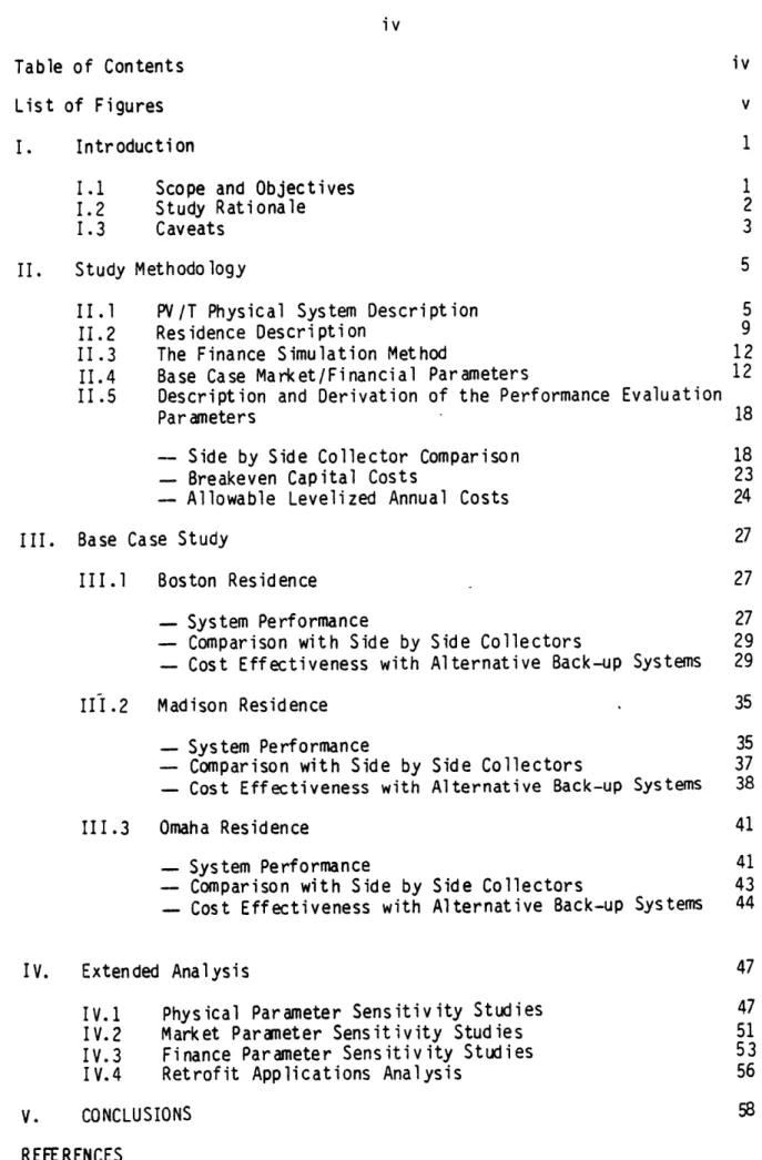
Table of Contents iv

List of Figures v

I. Introduction 1

I.1 Scope and Objectives 1

1.2 Study Rationale 2

1.3 Caveats 3

II. Study Methodology 5

II.1 PV/T Physical System Description 5

11.2 Residence Description 9

11.3 The Finance Simulation Method 12

11.4 Base Case Market/Financial Parameters 12 11.5 Description and Derivation of the Performance Evaluation

Parameters 18

-- Side by Side Collector Comparison 18

- Breakeven Capital Costs 23

-- Allowable Levelized Annual Costs 24

III. Base Case Study 27

III.1 Boston Residence 27

- System Performance 27

-- Comparison with Side by Side Collectors 29 - Cost Effectiveness with Alternative Back-up Systems 29

111.2 Madison Residence 35

- System Performance 35

- Comparison with Side by Side Collectors 37 - Cost Effectiveness with Alternative Back-up Systems 38

111.3 Omaha Residence 41

- System Performance 41

- Comparison with Side by Side Collectors 43

- Cost Effectiveness with Alternative Back-up Systems 44

IV. Extended Analysis 47

IV.1 Physical Parameter Sensitivity Studies 47

IV.2 Market Parameter Sensitivity Studies 51

IV.3 Finance Parameter Sensitivity Studies 53

IV.4 Retrofit Applications Analysis 56

V. CONCLUSIONS 58

V

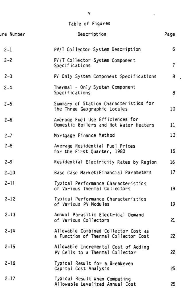
Table of Figures

Figure Number Description Page

2-1 PV/T Collector System Description 6

2-2 PV/T Collector System Component

Specifications 7

2-3 PV Only System Component Specifications 8 2-4 Thermal - Only System Component

Specifications 8

2-5 Summary of Station Characteristics for

the Three Geographic Locales 10 2-6 Average Fuel Use Efficiences for

Domestic Boilers and Hot Water Heaters 11

2-7 Mortgage Finance Method 13

2-8 Average Residential Fuel Prices

for the First Quarter, 1980 15 2-9 Residential Electricity Rates by Region 16 2-10 Base Case Market/Financial Parameters 17 2-11 Typical Performance Characteristics

of Various Thermal Collectors 19 2-12 Typical Performance Characteristics

of Various PV Modules 19

2-13 Annual Parasitic Electrical Demand

of Various Collectors 21

2-14 Allowable Combined Collector Cost as

a Function of Thermal Collector Cost 22 2-15 Allowable Incremental Cost of Adding

PV Cells to a Thermal Collector 22 2-16 _{Typical Result for a Breakeven}

Capital Cost Analysis 25

2-17 Typical Result When Computing

Table of Figures (continued)

Figure Number Description

Boston 2-18 2-19 2-20 2-21 2-22 2-23 2-24 2-25 2-26 2-27 2-28

Collector Thermal Performance Characteristics

Collector System Electrical Performance Characteristics

Collector System Parasitic Electrical Demand

Allowable Combined Collector Costs Allowable Solar Cell Cost

Combined Collector BECC for Each Backup Type

System BECC Comparison for Backup

System BECC Comparison for Backup

System BECC Comparison for Resistance Backup

Oil as

Gas as Electric

System BECC Comparison for Heat Pump as Backup

Allowable Levelized Annual Cost the Combined Collector System

for Madi son

Collector Thermal Performance Characterist ics

Collector System Electrical Performance Characteristics

Collector System Parasitic Electrical Demand

Allowable Combined Collector Costs Allowable Solar Cell Cost

Page 2-29 2-30 2-31 2-32 2-33

vii

Table of Figures (continued) Figure Number 2-34 2-35 2-36 2-37 2-38 2-39 Omaha 2-40 2-41 2-42 2-43 2-44 2-45 2-46 2-47 2-48 2-49 2-50 Description

Combined Collector BECC for Each Backup Type

System BECC Comparison for Oil a Backup

System BECC Comparison for Gas a Backup

System BECC Compari Resistance Backup System BECC Compari Backup

s

s

son for Electric son for Heat Pump as Allowable Levelized Annual Cost

the Combined Collector System

Collector Thermal Performance Characteristics

for

Collector System Electrical Performance Characteristics

Collector System Parasitic Electrical

Demand

Allowable Combined Collector Costs Allowable Solar Cell Cost

Combined Collector BECC for Each Backup Type

System BECC Comparison for Oil as Backup

System BECC Comparison for

Backup

Gas as

System BECC Comparison for Electric Resistance Backup

System BECC Comparison for Backup

Heat Pump as Allowable Levelized Annual Cost for the Combined Collector System

Page

Figure Number

viii

Table of Figures (continued) Description

Sensitivity to Cell Reference Efficiency Sensitivity to Thermal Storage

Volume

Sensitivity to Gas Hot Water Heater AFUE 2-51 2-52 2-53 2-54 2-55 2-56 2-57 2-58 2-59 2-60 2-61 2-62 2-63 2-64 0 0 0 0 tE 0 0 o

il Hot Water Heater AFUE Gas Boiler AFUE

Oil Boiler AFUE

Annual Price Escalation

s

Inflation

Time of Day Electric Homeowner Discount Rate Marginal Tax Bracket Mortgage Interest Rates Down Payment on the Sensitivty to Sensitivity t Sensitivity t Sensitivity t in Utility Ra Sensitivity t Sensitivity t Utility Rates Sensitivity t Sensitivity t Sensitivity t Sensitivity t Mortgage Sensitivity t Page

I. INTRODUCTION

1.1 Scope and Objectives

The specific focus of this study is to establish the cost goals required to make residential photovoltaic/thermal collector systems economically competetive with conventional and other non-conventional energy systems. Combined photovoltaic/thermal collectors, hereafter

referred to as PV/T or combined collectors, are compared with separate PV and thermal collector systems set side by side, and with PV alone. Each system is evaluated against four alternative means for satisfying the thermal portion of the residence load: all oil, all gas, all electric resistance, and electric resistance hot water with space heating by parallel heat pump. In each case an electric vapor compression unit was modeled for summer space cooling.

This study develops a base case set of market and financial parameters with which to simulate the cash flows for a PV/T investment starting in 1986 in each of three northern locations: Boston, Madison, and Omaha. The base case analysis includes a newly constructed residence equipped with boiler and heater units having efficiencies anticipated for

1986. The PV/T collector is of a flat-plate, liquid cooled design. An optimally sized collector system is then chosen for Boston where

sensitivity studies are performed to selected physical, market, and financial parameters. In this extended analysis, a retrofit application

is characterized and compared with the results for a newly constructed home.

1.2 Study Rationale

Combining the functions of solar photovoltaic and thermal collectors into a single module design is conceptually attractive for many reasons. First, the cost of a combined collector module should be markedly less than for separate collectors when added, since many of the

collector components, e.g. glazing, substrate materials, support structures, shipping and installation costs, etc., are common. Also, combining the two functions strives to maximize the energy output over

the often limiting variable of rooftop area.

Although such a combination has the potential to displace significantly more conventional fuel as does an equivalent area of separate collectors, the latter is not necessarily equivalent to the objective of an economically rational invester. For this reason, recent studies have either challenged the Department of Energy's impetus in PV/T development (see Hoover, 9) or have severely qualified the realm of application (See Russell, 11). Specific problems identified as limiting the viability of PV/T systems include:

o deleterious interactive effects of combining the functions of the two collectors. Thermal collectors are designed to absorb and transport maximum quantities of heat with large discrepancies in seasonal demand. Photovoltaic output, on the other hand, is inversely correlated with temperature, and utilizable

year-round. For this reason, combined collectors are generally less efficient and have larger parasitic electrical demands for heat rejection in summer months1

1_{Hoover (9) reports that, in a southern location, roughly three}

quarters of the combined collector area is required by PV-only for an equivalent electrical output.

o the optimal size of the two collectors are usually different. Photovoltaic systems, especially when supported by high rates for utility buy back, are optimally sized for much larger areas than are required for thermal output. Northern locations, with larger proportional thermal loads, are expected to improve PV/T worth for this reason.

Furthermore, Russell (11) has reported that, of series and parallel heat pump options for auxiliary thermal energy, parallel systems prove more cost effective. He also points out that, excepting breakthroughs in

storage technology costs, on-site electrical storage leads to sub-optimal designs, Dinwoodie (8) and Caskey (6) offer detailed analysis to support this latter point.

All of the above were considered when formulating the objective, scope, and system description of this study.

1.3 Caveats

We wish to stress from the start the limitations inherent to this analysis. To start, our results derive from the use of a model

describing one liquid-cooled PV/T collector design. The extended analysis portion examines the impact of variations in single physical parameters such as electrical efficiency, thermal emissivity, and storage tank volume, however the basic system configuration is left unchanged. Our results, therefore, apply only to the collector system as described in the next section. Secondly, the individual components of the

collector system, such as pumps, storage tank, heat exchangers, and so forth, have been sized with engineering optimizing

4

objectives, and not according to any form of operational cost

minimization formula. The latter objective would obviously lead to improved system worth.

With regards to the base case economic analysis, it was debated whether to estimate required cost goals based upon the unsubsidized merit of system worth, or to assume market conditions for 1986 as an

investor would see them. This would include, in all likelihood, some form of investment tax credit. The decision was to not model the tax credit. Since we are using prices for electricity, gas, and oil at expected deregulated prices beginning in 1986, the figures in the base case analysis represent costs which must be met in order to be

competitive and unsubsidized prices. Any reasonable value for investment tax credit would be reduced from its current (1980) offering of 40

percent or $4,000 (maximum). Solar tax credits tend to come in solar packages with maximum credits applicable to the sum of solar investment options. Thus the "marginal" credit to a PV/T or some combination of PV

and T would be something less than the maximum, given credits for passive design, a solar greenhouse, or other investor options. Of all things one may be sure of, the tax credits scenario for 1986 will be unlike what we see now. A sensitivity study to this important parameter is conducted in the extended analysis.

The final caveat to be mentioned here regards the use of residential loads which are established without consideration of the impact of other technologies, especially load management, upon the load profile. In an analysis of the impact of time of day rates upon PV/T worth, this fact may be important.

II. STUDY METHODOLOGY

II.1 PV/T Physical System Description

The PV/T collector system evaluated here is depicted in

Figure 2-1. Since this system is assumed to run parallel to each backup system considered, there is little complication in defining precisely those components included when establishing allowable initial costs.

These components include:

o PV/T solar collector

o thermal storage tank

o pre-heat storage tank

o all pumps

o heat rejection equipment

o assembly

o all distributor and manufacturer markups

o installation costs

o warranty costs

These "initial" costs are included in the breakeven capital cost figure, as calculated in section 11.5. The allowable levelized annual costs figure includes, in addition, all annual costs as follows:

o annual insurance o operation

o maintenance

The performance models describing the operation of the PV/T collectors, in addition to the PV and thermal-only collectors, were

developed by Raghuranan at Lincoln Laboratory. System integration

utilizing TRNSYS components was accomplisyhed by Russell, also at Lincoln Laboratory. Implementation of these models on the Optional Energy

Systems Simulator2 _{(OESYS) was carried out by the authors.}

Pertinent parameters describing system components are presented in Figure 2-2. Characteristics of the separate PV and thermal collectors are described in Figures 2-3 and 2-4, respectively.

I! " -- Controller--' Controller

Heat Rejection

Figure 2-1

Figure 2-2

PV/T Collector System Specifications Collector Characteristics:

FLAT PLATE

non-concentrating

liquid-cooled

single-glazed laminar tube flow

cell packing factor (total cell area/gross coll. area)

cell envelope area/gross coll. area

tilt angle (deg)

gap cell thickness (cm) potant thickness (cm)

Outer dia. of tube (cm)

Absorber plate thickness (cm) inner dia. of tube (cm)

potant conductivity (Wcm-1 °C-l)

absorber plate conductivity (Wcm-_{l *C}- 1

)

cell emissivity

cell IR absorptivity

glass emissivity

cell visible absorptivity

glass transmissivity potant transmissivity

absorber visible absorptivity

cell reference efficiency

cell efficiency temperature coefficient (*k-l)

cell efficiency reference temperature (oC)

specific heat of liquid (Joules kg- OC'')

length of cell envelope area (cm)

number of tubes in collector

thermal conductivity of liquid (Wcm-1 OC-1)

Storage Tank Characteristics

storage mass/collector area (kg/m2)

tank height 9m0

specific heat (kJ/kg - °C)

fluid density (kg/m)

heat loss coefficient (kJ/hr-m2 - oC)

.90 .9 latitude + 50 1.0 .05 1.6 .08 1.27 .012 2.0 .10 .10 .86 .89 .92 .85 .95 .135 .0045 28. 4186. 231. 7. .0059 50. 2. 4.186 1000. 1.5

Figure 2-3

PV-Only System Component Specifications

Glass thickness (cm) encapsulant thickness

outermost substrate thickness (cm) conductivity of glass (w/cm*C) conductivity of encapsulent (w/cm°C) conductivity of substrate (W/cmOC)

r, product of cell

TI product between cells

emissivity of glass

emissivity of back surface

packing factor (total cell area/gross cell area IR absorptivity of glass

IR absorptivity of back surface visible absaorptivity of roof

IR absorptivity of roof emissivity of roof

reference cell efficiency Eff. charge coefficient

reference temperature for ref cell efficiency (OC)

mounting angle from horizontal

.32 .15 .10 .0105 .00173 .01 .8 .75 .88 .9 .90 .99 .9 .6 .903 .903 .135 .0045 28. latitude + 5' Figure 2-4

Thermal-Only System Component Specifications collector efficiency factor

fluid thermal capacitance (kg/kg OC)

collector plate absorptance

number of glass covers collector plate emittance

loss coefficient for bottom and edge losses collector tilt angle (degrees)

transmittance .95 3.35 .10 1.06 latitude + 5o .9

11.2 Residence Description

The residence energy loads are divided into stochastic electrical and thermal (weather-dependent) loads. The stochastic load profile is a probabilistic description of household electrical appliance demand

obtained from the Residential Electric Appliance Simulator (REAS).3

The weather dependent loads were obtained from a General Electric model of a detached, northern climate, two-level single family house (See

Scollon. 12). _{The weather data included a typical meteorological year in} each location, and the'solar technologies were modeled using hour by hour matching for the same weather year. A summary of station characteristics for each of the three loactions are presented in Figure 2-5.

Thermal energy demands for space heating and hot water were satisfied by several conventional sources while supplemented by the PV/T collector output. THe conventional backup alternatives modeled in this analysis include:

o _{gas space heating, vapor compression cooling, gas hot water}

heating

o _{oil heating, vapor compression cooling, oil hot water heating} o electric resistance heating, vapor compression cooling, electric

hot water heating

o _{parallel connected heat pump for space heating and cooling,}

electric resistance hot water heating.

3

Developed at the M.I.T. Energy Laboratory by William A. Burns and described in (5).

I 31WullA 13W'1OS NI 03ION SV 0 OOI3J 016-iV61 NO 03SVG 4 'eC I t 16!; 6 '60!; 4 'ZZV 0*9c,1 o'zosl 0 *v1611 O 1906cr 0 '9396! 0 b68sci O !;6IOL G 11!; I VVt9 8 16V0I VECC Mt8!S 990 1Z !15 ZT 9'Z481 t I 8!;!;1 !; 'ZU1 1 '7-60 Olt 7099 66 01 4 91 9011 4.C 1 z *C6z V 'In. 6' 09 01*0!; 9 1 fi !; .sz 16C 0'61 SC9 z 109 s* *0!; 6 l8e I110Z; 1 '91 Elr1 it 6r. c *!;s * I IL 0 19 1 Vi* sA3'i0nV zw./rx zid/ruS

ONOIOIWN NVIOS A 1IWO NV3W 3jw3Hds1IaN '1v±ca

ONY1000 ONI.LV3H A'1HINOW UflUINIW WrIWZXVW H.LNOW

A 030 !;9 asV6e AIM1V A-1ic

OsAti0 33V030 'WWWM

o(i 030) 3Wfl±WU3dW31 1VW)5ON

tot IN0I±VA313 M11096 130ami0Noi NZu1* t3aruiivif 8166 si

31 : 31tols VHW0 HidON :NOZ.LVJS

I BWMlOA iaww1s ni 03±oN sw #

0 *Cz:c I *t6bz C'Z4V I *Soc I 'SIZ S* 6C1 0 '7*6* 1 O'c"Te6 0'0827 0 *31.6 OISZ;16 0 1 6*8!; 610611 6 on8 6 '016 1 '8041 * '*361 Z'Cfp41 * '86c1 0 '*08 13GWflN NOI.W±S *******"I I GOINU. OL6T16l NO 03StlG 09V 0 0 9 Z1 96 at 0 0 0 0 606 *L* C41 63-16.10 6L0 I zrw 1 06V I 6 It*r 6 '6!; 1 *01 0 '9!; C Is* z *03 C '0z 819T 0 *I *3 Ca 6e!; 9 1 V1 9 1)T VIC8 0'!;!; a 16Z 6 *09 0108 0 *9s * 6c r,16 v Iroz NNV 33a AON 130 d3S vnw 9A#W Nw'

sA3,iaNri z14/P)I u±j/ls

0H0I±V1CVdS W-0S A'lW NV3W~ OIUBH'4SIW3H -W.01

DNI1003 ONJIVSH AIHINOW

a 030. 29 MoeS *SA*8a 33WO3a 'IWW0N

WnfWINIW WfM.IXWIHLNO4 Allitt Alive

*(A 030) 3WUM1VH34d1 'IWbWON

z : N0I±tfA3-G M0Z68 330floINol Nsocv :30fLLIVI 658* *I36WN NOZIVIS

7 3WnFiOA 13:410S 41I 03.LON SW 0 0III3 0661-1*61 NO O3SV 9 1'6.6 C '601 V*9C 9'6; 0 ' 65 0'4C!;Z1 0 1 WQVO 0 '560'T 0'04891 0 '9t 02 1 n *V!; IT 0 '96F!; 6 1 z0r I '41S8 916049 8'24t3 199 0 0 0 19 C0z 09Z '411 0 0 0 U~6 94 0 U6tp 01 VI C 'St 0' 09 9 *sr. 91st I' l0e V '65 a let 94'92 6 '53 1 '09 reI 'C 8'* ra *zC C *64 9'94 1 '69 NNVt :330 AOt4 ±30 CGS Im Nnr AWU 13A

SABIONVI U/I'J/r cl/l±is

ONC'±VIMA Nv'1os A'111i Nv3I4

31j3id.1W3H '1V±0±

t3NI')O3 ONI±V3H AJN±NOUW Wi)WINIW WM1IXtOW H±LNOW

j Ca'] 59 BSVB A1V0F A,1IVO1

*sAtoo 33*1030 IWU*ON

*(A 030) 3uiVSS3i -WWWIO

S :14011VA313 t Z016 z30l'l±I01 NZZIt :30fl11±IJ1 104V6 :V38WAN NOJIVIS

vw& :31viS NOiSC'8 :N0I±W±S

S:)LSL.JBJ)RLP4 UOL;4S 40

i('ipwwfl

S-Z a.fl6LI

000"0* 4*6

im S31WIS NOSIOVW Wolivis

11

The boiler and heater efficiencies used in this analysis were derived from telephone conversations and literature research directed at unit efficiencies likely available for 1986 installation. These

efficiencies, in terms of overall average fuel use, are depicted in Figure 2-6. Sensitivity runs were performed on these parameters in the extended analysis.

Figure 2-6

Average Fuel Use Efficiencies for

Domestic Boilers and Hot Water Heaters 1986 Technology

Boilers Average Fuel

TYPE Use Efficiency Efficiency Range

OIL* 81% 70-90% GAS** 69% 60-80% Electric Resistance 100% Hot Water OIL 60% 45-65% GAS 60% 50-70% Electric 86% 80-90%

*taken from the upper range of currently available efficiencies as listed in (13).

**telephone conversation with Charles Steats, Bradford Wright Corp. 7/29/80 these numbers were confirmed as reasonable by others in the field.

12

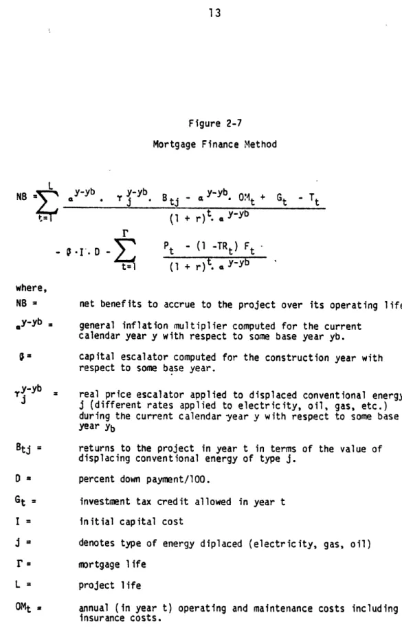
11.3 The Finance Simulation Method

Finance modeling was carried out on the Optional Energy Systems Simulator (OESYS)4 _{using a cash flow analysis of a standard}

homeowner mortgage. The method used is depicted in Figure 2-7. Here, we compute the system breakeven capital cost by determining that initial cost, I, where the net benefits just equal zero. Simulating annual cash flows differs from closed form solutions in its accountability of time varying inflation, fuel escalation, and tax rates, in the treatment of

investment tax credits, and in determining tax benefits due to

time-varying interest charges. Comparison and assessment of the various homeowner finance models currently being applied to photovoltaic

investments is discussed by Cox (3).

11.4 Base Case Market/Financial Parameters

Those parameters which are independent of the solar investment but which directly impact the prospects for that investment are listed here as market parameters. These include fuel and electricity prices for backup service, time-varying escalation rates applied to these prices, the general inflation rate, and others. The values assumed for these parameters are listed in Figures 2-8 through 2-10.

Figure 2-10 also presents a conservative set of base case parameters effecting project finance. The zero value assumed for an investment tax credit in 1986 allows an unsibsidized allowable cost to be computed. A discussion of this is found in section 1.3. Figure 2-10 also presents system annual costs used in the breakeven capital cost analysis. The breakeven capital cost figure represents the initial

allowable system cost only.

4

Developed by T.L. Dinwoodie at the MIT Energy Laboratory.

---13

Figure 2-7 Mortgage Finance Method

NB L y-yb -yb. tj .y-yb. Ot + Gt .Tt

(1 + r)t. * y-yb

r

- -t - (1 -TRt) Ft

t= ( + r). yyb

where,

NB = net benefits to accrue to the project over its operating life

Gy-yb = general inflation multiplier computed for the current calendar year y with respect to some base year yb.

r= capital escalator computed for the construction year with

respect to some base year.

Ty-yb real price escalator applied to displaced conventional energy j (different rates applied to electricity, oil, gas, etc.) during the current calendar -year y with respect to some base year yb

Btj = _{returns to the project in year t in terms of the value of}

displacing conventional energy of type j.

D = percent down payment/100.

Gt = _{investment tax credit allowed in year t}

I = initial capital cost

j = _{denotes type of energy diplaced (electricity, gas, oil)} I = mortgage life

L = project life

OMt = annual (in year t) operating and maintenance costs including insurance costs.

14

Figure 2-7 (cont'd)

r = homeowners discount rate

t = project year

Tt = sum of taxes in year t

TRt = homeowner's tax rate in year t

Ft = mortgage interest charge in year t computed as Ft = A - Pt, where;

A = annual mortgage payment, given by

A = I . (1 - D) . (i/[l - 1/(1 + i))N])

i = annual mortgage rate

Pt = payment required on the balance of principle in year t, from

Pt i . BALt, where

Figure 2-8

Average Residential Fuel Prices for the First Quarter, 1980

Heatinq l .ra QaAl

(cenH tper a on) (do as e all ion)

BTU's

1980 1986# 1980 1986+

Price Adjusted Price Adjusted

Price Price

(1980 $) (1980 ;)

NEW ENGLAND 96.7 116.04 4.92 8.12

(Boston)

EAST NORTH CENTRAL 93.5 112.20 3.16 6.32

(Madison)

WEST NORTH CENTRAL 93.6 112.20 2.79 5.58

(Omaha)

+ The 1986 price is the 1980 price adjus.ted for deregulation. For oil

this is given by a 20% increase over the 1980 price. For natural gas,

this is given by either price doubling or the cost of gas at an

equivalent BTU content of oil at the adjusted price, whichever is

minimum. Estimates for deregulation of gas prices suggest these prices will double, but it is unlikely that they will exceed the cost of deregulated oil on an equivalent energy content basis.

* Source: Energy Data Report DOE/EIA - 0013(80/03)

Figure 2-9

Base Case

Residential Electricity Rates by Region* (Based on Average 600 kwh/month Usage)

Boston Fixed Charge per kwh/charge fuel adjustment $1.17/month 3.954/kwh 3.905s/kwh 7.86e/kwh Madison Fixed charge per kwh/charge fuel adjustment $2.50/month 4.14/kwh $ .52C/kwh 4.66/kwh Omaha Fixed charge per kwh/charge fuel adjustment $3.95/month 3.64e/kwh .208t/kwh $3.85/kwh

* Source: Correspondence with the electric

Figure 2-10

Base Case Market/Financial Parameters and Annualized Costs

Market Parameters

Escalation in Home Heating Oil Prices (real)

Escalation in Gas Prices (real)

Escalation in Electricity Prices (real) General Inflation Rate

Utility Buyback Rate

Finance Parameters

System Installation Date

System Lifetime

Homeowner Discount Rate (real) Homeowner Tax Rate

Mortgage interest rate (real)

Down payment

Investment tax credit Property taxes 2%/year 2%/year 1%/year 12% in 1980, declining linearly to 6% in 1986, 6%/year thereafter .80 1986 . 20 years 5% 35% 3% 10% 0 0

Cleaning and Inspection

Annualized Costs (Annual Cost) PV-only system* PV + T side by side# Combined Collector# Maintenance PV-only System PV + T Side by Sidg#+ Combined Collector; $25 + $1.00/m2 $25 + $1.00/m2 $25 + $1.00/m2

(Present value at 5% discounting)

$13.00/m2 $13/m2PV + $62 + 5.00/m2T

$62 + $18/m2

Insurance (Annual Cost)

All systems $30 for first 5K of system cost; $2/lk each additional Ik

* See Cox (7).

# Obtained from telephone conversations with solar-thermal Installers. Most influential was Lou Boyd, Solar Solutions, Inc., Natick, MA.

Maintenance costs were broken down into annual checkup and expected (1986) component failure probabilities coupled with the probability of the cost of repair.

18

11.5 Description and Derivation of the Performance Evaluation Parameters

Three figures of merit are utilized in this analysis, each of which assesses an allowable system cost. These include an allowable

combined collector cost for comparison with side by side collectors, a

breakeven capital cost, and an allowable levelized annual cost. They are taken in order here.

Side by Side Collector Comparison

This analysis follows directly from a study conducted by Hoover(9) addressing those conditions under which a flat plate PV/T

collector can compete with separate photovoltaic and thermal collectors. This method determines the allowable combined collector cost given

1) the cost of PV and thermal collectors, and 2) the separate PV and thermal array areas required to produce electrical and thermal output equivalent to the combined collector. Derivation of allowable combined

collector cost is given by the following example

The thermal performances of a combined collector and two thermal collectors are shown in Figure 2-11. This figure suggests that 13 m2

of a thermal collector with 10 percent infrared emittance, the same emittance modeled for the combined collector, yields a solar fraction equivalent to 40 m2 _{of combined collectors. Emissivities}

characteristic of non-selective surface thermal collectors are around 80 percent, which requires roughly 26 m2 _{for equivalent output.}

Figure 2-12 presents the electrical output characteristics of ohotovoltaics-only verses that of a combined collector. Output from the latter has been reduced by the parasitic electrical requirements of the collector pump and of the heat rejection unit.

ION OF TOTAL HOT WATER ANO HERTING LORD MET BY SOLAR

O THERMAL COLLECTOR = . 10

0 THERMAL COLLECTOR * = .80 Q COMBINED COLLECTOR

TOTAL COLLECTOR AREA (M2)

Figure 2-12

TOTRL COLLECTOR SYSTEM ELECTRICAL

OUTPUT (RANNUAL) O PV ONLY O COMBINED COLLECTOR Figure 2-11 FRRCT SPRCE 0 0 z c U. cccx -, (n 8 In a Y N a LLI LJ 0 0

20

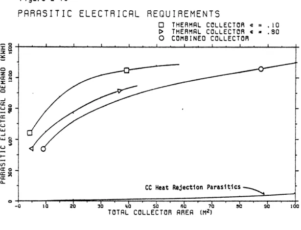
Figure 2-13 next illustrates the parasitic electrical demand placed by the various collectors. The difference in parasitic demand between 40

m2 _{of combined collector and an "equivalent" area of thermal}

collector (e = .80 at 26 m2_{) is 1000 kwh. Adding this to the}

combined collector output of Figure 2-12 is necessary in order to compare directly with the net output of an equivalent side by side PV and thermal system. (Equivalently, this difference in parasitic demand is subtracted from the gross output of a PV-only system to reflect that energy which went toward satisfying the parasitic demand of an accompanying thermal system.)

Thus, if we add 1000 kWh to the net annual electrical output of the combined collector (on Figure 2-12), we find that the equivalent PV-only is roughly 27 m2. Assuming a cost for both a photovoltaic

module and thermal collector allows computation of the maximum allowable combined collector cost by the following relationship:

A A

AC

_-ccA-

_CpT

CC

CC

where

ACCC = allowable cost for the combined collector, $/m2

ApV . equivalent PV collector area, m2 ACC = combined collector area, m2

ATC = equivalent thermal collector area, m2

CPV = PV module cost, $/m2

= Thermal collector cost, $/m2

Figure 2-13 PRRRSITIC ELECTRICRL IE: Z8 CcNX _~j Cr U O LJ Cr0 ccI 0J I--U, 0co 0C REQUIREMENTS 0 THERMRL COLLECTOR a = .10 > THERMAL COLLECTOR .80 O COMBINED COLLECTOR

For our example, we fix the PV cost at $70/m 2 and, in

Figure 2-14, plot the allowable combined collector cost as a function of thermal collector cost. We see that for a selective surface thermal collector cost of $100/m 2 _{and PV module at}

$70/m 2, the allowable cost for the combined collector is $90/m 2. By assuming that the thermal collector portion of the combined collector costs the same to manufacture as a separate thermal-only system, we can determine the

allowable incremental cost for adding PV cells to the thermal collector. This is accomplished in Figure 2-15 by subtracting a line of slope 1 from the lines of Figure 2-14. For thermal collector costs above $160/m 2

we could not afford to pay anything for the addition of PV cells. The latter methodology, leading to Figures 2-14 and 2-15, are taken directly from Hoover's analysis and utilized in this report when comparing PV/T with side by side collectors. It is important to note the

Figure 2-14

RLLOWRBLE COMPARING

COMB

SIDE

MODULE COST S= .80 S= .10 Figure 2-15 INCREMENTRL FOR COMBINED 0 lo ,, c: 3= CL 9-, C 0T 03 -J~ RLLOWABLE PV COST COLLECTOR PV MODULE COST AT s70/M2 0 4 - .80 0 4 = .10 AT $70/M2 o o N X: 1-= V), 0 L_)

Li

23

shortcomings of this method, many of which are outlined by Hoover (9). First, this technique holds that the proportional electrical vs: thermal output of a combined collector is maintained by side by side collectors.

In fact, the optimum relative areas of separate PV and thermal collectors may be quite different from the "equivalent" areas, and hence the

separate collector system may prove significantly more attractive than the computed "allowable" PV/T costs suggests. We attempt to resolve this problem by including varying PV and thermal collector area ratios when comparing side by side with combined collectors in the breakeven cost analysis.

Furthermore, this analysis does not consider the cost of a heat rejection unit required by the combined collector system, and the size of the thermal system components, especially collector punps, piping, and the storage tank, would be less than for the combined collector system. These costs may or may not be offset by the reduced cost of installation of a single collector system.

Breakeven Capital Cost

The method used to compute the collector system breakeven capital cost was presented in Section 11.3. Figure 2-16 illustrates how this quantity is depicted in this analysis. Since our base case analysis uses a 5 percent homeowner discount rate, multiplication of all figures shown by .0802, the capital recovery factor for a 20-year life at 5 percent, yields an equivalent allowable'levelized annual cost under the given

financing conditions.

To arrive at the familiar $/Wp, the vertical axis can be divided by the overall array efficiency times 1000 W/m2 standard peak

24

times the array packing factor times the front panel reflectance. For our base case analysis, this figure is .014, so that the total divisor is 104.

Allowable Levelized Annual Cost

This figure is arrived at as a function of collector area but independent of all financial parameters excepting the investors discount rate and the rate of inflation. It is calculated as the equivalent

annual payment which results from applying a capital recovery factor to the sun of discounted yearly payments. The conventional manner for computing capital recovery factor is given by

CRF = r'(1 + r')

(1 + r') N

1

In order to arrive at a capital recovery factor in constant (base year) dollars, as opposed to current year (nominal) dollars, we calculate the discount rate r' to be the real (or inflation adjusted) discount rate, defined as

r' = l+r 1

where g is the general inflation rate.

Estimation of this relationship is depicted in Figure 2-17. Curve A is the levelized annual cost to the homeowner of satisfying all residence energy demand by conventional means, in this case, all oil. It is the levelized annual cost of all heating oil and electricity as billed by the utility. Curve B is the same levelized annual cost as presented by utility bills, but with a solar system supplementing. The difference between these two _{curves, Curve C, is that levelized annual cost which a} homeowner may be willing to pay for that solar system. Since the

Figure 2-16 SYSTEM BREAK OF ALTERNRTI BACKUP: GAS o o a IuJ EVEN CAPITAL VE COLLECTOR COL 0_0] COSTS COMPARISON SYSTEMS LECTOR SYSTEM: PV ALONE PV*T (75/25) PV+T (50/50) Figure 2-17

ALLOWABLE LEVELIZED ANNUAL COST ANALYSIS

BACKUP PROVIDED BY:

O ELECTRIC RESISTANCE 0 HEAT PUMP 5% Discounting 0 OIL A GAS. 0 0 'I -J

26

homeowner is assumed to pay monthly energy bills out of hand (not by borrowing), only his/her rate of discount of future cash payments enters

into the investment decision. However, computation of the solar system levelized annual cost, for comparison with this allowable costs figure, must account for the effects of borrowing.

There is an important distinction to be made between the system breakeven capital cost and the allowable levelized energy cost as

presented here. First, those costs which these figures take account of differ, as described in section II.1. The system BECC only accounts for all first-year costs, not annual costs. Second, the system BECC takes into account financing, and for the base case financial parameters

assumed, this figure yields a higher levelized annual cost than the ALAC method. There are two reasons for this. First, setting the discount rate higher than the mortgage interest rate results in having acquired a

loan with a positive net value to the borrower. Second, the tax effects of borrowing improve system worth by offering deductions on the interest

payments. If, in the system BECC formulation, the tax rate is set to zero and the discount and interest rates set equal, application of the capital recovery factor to the total system BECC should result in the

ALAC computed by the alternative method. Since in our formulation of the 8ECC we subtract out all annual (0 and M plus insurance) payments, our levelized annual cost computed from the BECC is lower than the ALAC by just the equivalent levelized annual 0 and M costs assumed. This has provided an important check on our results.

The allowable LAC curve represents costs below which the

levelized annual costs must lie, however they may be financed. This is the attractive feature of the ALAC formulation. One is free to choose

his or her own finance parameters (down payment, tax credit, interest rate, etc.), remaining consistent only with the discount rate and utility price escalation rates assumed.

III. BASE CASE STUDY III.1 Boston Residence

Typical annual meteorological conditions were depicted for Boston in Figure 2-5. These conditions translate into the following annual

house loads:

Space Heating: 33.285 MBtu's Space Cooling: 4.012 MBtu's Hot Water Heating: 16.776 MBtu's

In addition, the residence had a non-weather-related stochastic electricl load which summed to 5886 kWh for the year. This latter figure does not include the parasitic electrical demand of the solar collector system.

System Performance

Figure 2-18 compares collector system thermal performance characteristics. The vertical axis is the fraction of solar system supplied hot water and space heating load over the total house space heating and hot water load. Figure 2-19 presents the electrical output characteritics of both a PV-only and PV/T collector system. The PV/T system output is shown reduced by its parasitic electrical requirement. Parasitic electrical requirements for both thermal and combined collector systems are plotted as a function of collector area in Figure 2-20.

The various economic figures of merit utilized in performance evaluation were described in section II.5. They are examined here in

TOTRL HOT WATER RNO

NG LORD MET BY SOLAR

o THERMPL COLLECTOR c

O THERMAL COLLECTOR = < COMBINED COLLECTOR

TOTAL COLLECTOR AREA (M2)

Figure 2-19 TOTAL COLLECTOR OUTPUT (ANNUAL) SYSTEM ELECTRICAL BOSTON 0 PV ONLY 0 COMBINED COLLECTOR Figure 2-18 FRRCT SPACE ION OF HEATI BOSTON .10_.80 z U cc U-c. cr 0 U, iv 0 U, c I-I--_r cc 0 W 0 o 0-0 a

29

Figure 2-20

PARASITIC ELECTRICAL REQUIREMENTS

0 THERMAL COLLECTOR 4 = .10

BOSTON > THERMAL COLLECTOR 4 = .80

O COMBINED COLLECTOR

4cx

g-CC Heat Rejection Parasitics

-o 10 20 30 (o 5so O 70 36 90 O

TOTAL COLLECTOR ARER (M2)

Side-by-Side Co l lector Comparison

Allowable combined collector costs, as defined in section II.5,

are shown plotted in Figure 2-21. Figure 2-22 depicts the incremental

allowable combined collector cost. We find that we could afford to pay

zero dollars for inclusion of the solar cells if the thermal collector costs were greater than $80/m 2 , when comparing with side-by-side

systems having selective surface absorbers. Since flat-plat selective

surface collector costs range typically from $80-$150/m2 , this

analysis does not appear to favor combined collector systems for Boston.

Cost Effectiveness with Alternative Backup Systems

The combined photovoltaic/thermal collector system is modeled in

tandem with each of the four types of conventional backup systems and a

30

through 2-28 allow comparison of PV/T with PV-only and side-by-side collector systems, again for each backup type. Careful attention should be paid to the vertical axis divisions, as these change on each graph. Breakeven costs are nearly identical when modeling oil and gas backup systems since the cost of these fuels was set equal on a Btu-equivalent

basis (see Figure 2-8). This is not found to be true for the Madison and Omaha runs, where gas prices tend to be lower. The high electric rates

in Boston (double those of the other two cities) prove PV-only systems twice as attractive as in the other cities, and cause all collector systems to be most attractive when electric resistance is the only means of space heating available. These plots clearly portray that the thermal collection portion is optimally sized to an area smaller than the optimal electrical portion.

The system breakeven costs curve for the combined collector

system is always below that of at least one of the side-by-side collector systems for the range of total collector areas modeled. Thus, one would always be able to pay some additional amount over the PV/T allowable cost in order to receive the energy benefits of some side-by-side

configuration. On the other hand, if the savings in assembly and

installation costs for the combined collector are significant, they may override the effects of poorer operational performance. The best

opportunity for this is in the 40-80 m2 _{range for the PV/T system.}

Finally, Figure 2-28 portrays the allowable collector costs, again as defined in section 11.5. The levelized annual costs of heating by oil, gas, or heat pump are remarkably close.

Figure 2-21

RLLOWRBLE COMPRARING

BOSTON

COMBINED COLLECTOR COST WHEN

SIDE BY SIDE PV RNO T COLLECTORS PV MODULE COST AT s70/M2

0 = .80

0 4 = .10

Figure 2-22

INCREMENTRL ALLOWABLE PV COST FOR COMBINED COLLECTOR

PV MODULE COST AT s70/Mz 0 I - .80 0 4 " .10 0 Xo I-N 0 -cc cr BOSTON a t in C. oU 0 -J -J

Figure 2-23

PV/T SYSTEM BREAKEVEN CAPITAL COSTS BACKUP PROVIDED BY: O ELECTRIC RESISTANCE

BOSTON _{O HEAT PUMP}

> GAS

S , i

1 ' 2z 30' u 50 50 70

PV/T TOTAL COLLECTOR AREA (M2)

s0 90

Figure 2-24

3TEM BREAKEVEN CAPITAL COSTS COMI RLTERNRTIVE COLLECTOR SYSTEMS

COLLECTOR SYSTEM: BOSTON 0 PV ALONE O PV+T 175/25) BACKUP: OIL A PV+T (50/50) PARISON L.J 0 ZI-U,>... N rj 0 0~

SYO

OF

--Figure 2-25

SYSTEM BREAKEVEN CAPITAL COSTS COMPARISON OF ALTERNRTIVE COLLECTOR SYSTEMS

COLLECTOR SYSTEM:

BOSTON 0 PV ALONE

O PV+T (75/25) BACKUP: GAS A PV+T (50/50)

SI I . ,O0 COMBINED COLLECT,OR

Figure 2-26

SYSTEM BREAKEVEN CAPI

OF ALTERNATIVE COLLEC

BOSTON

TAL COSTS COMPARISON TOR SYSTEMS COLLECTOR SYSTEM: O PV ALONE [ PV+T (75/25) BACKUP: ELECTRIC A PV+T (50/50) .0 COMBINED COLLECT.OR o o S O C.-,O uU, >.-0 N N 0 0O 0 ry U, C--r LU (,_(nr fy v 0

Figure 2-27

SYSTEM BRE

OF RLTERNR

RLLOWABLE

LEVELIZED

RNNUAL COST RNRLYSIS BACKUP PROVIDED BT: O ELECTRIC RESISTANCE Ol HEAT PUMP O OIL o oo U.J ?° LU (n )-0 UN N (.f' 0 0 0.,, a

111.2 Madison Residence

Figures 2-29 through 2-39 present results analogous to Figures 2-18 through 2-28 for the Boston residence. Discussion of these graphs will not be repeated here, but will be dealt with in the conclusions of section V. Again, pay careful attention to the vertical axis divisions of Figures 2-35 through 2-38. The Madison residence thermal loads are

summarized as follows:

Space Heating: Space Cooling: Hot Water Heating:

44.562 MBtu's

3.683 MBtu's 16.776 MBtu's

Figure 2-29

FRRCTION OF TOTRL MOT WARTER RNO SPRCE HERTING LORO MET BY SOLRR

C THERMAL COLLECTOR 4 = .10

MADISON 0 THERMAL COLLECTOR <( .80

4 COMBINED COLLECTOR z C a: a:Vc Cr I4

Figure 2-30 TOTAL COLLECTOR OUTPUT

ARNNUAL)

TOTAL COLLECTOR AREA 70 (M2) Figure 2-31 PARRSITIC MAOISON cr-z8 cr =_c LU -J 0 C, Q: 0 0c 0,

ELECTRICAL

REQUIREMENTS

TOTAL COLLECTOR AARER (M)

a- I-0 a: 0 _a ab Ib 00 90

Figure 2-32

ALLOWABLE

SIDE

INEO COLLECTOR C

COLLECTOR

Figure 2-34

PV/T SYSTEM BRERKEVEN CRPITRL COSTS

BACKUP PROVIDEO BY:

0 ELECTRIC RESISTANCE

MROISON O HEAT PUMP

A GRS I . I I , 0 OIL ,o C- U-0 Io-C 0, Iv-0 NoF 0e 0 0o 0-Figure 2-35

SYSTEM BRERKEVE

OF ALTERNRTIVE

N CRPITRL COSTS COMPARISON

COLLECTOR SYSTEMS COLLECTOR SYSTEM: O PV ALONE O PV+T (75/25) A PV+T (50/50) .0 COMBINEO COLLECTOR b ' 20 3 0tc so b ' sso 7 b d

Figure 2-36

SYSTEM BREAKEVEN CAPI

OF ALTERNRTIVE COLLEC MAOI3ON BACKUP: GAS TRL COSTS COMPARISON TOR SYSTEMS COLLECTOR SYSTEM: 0 PV ALONE O PV+T (75/25) A PV T (50/50) .0 COMBINED COLLECTOR

TOTAL COLLECTOR AREA (M2)

Figure 2-37

SYSTEM BREAKEVEN CAPITAL COSTS COMPARISON OF ALTERNATIVE COLLECTOR SYSTEMS

COLLECTOR SYSTEM: MAOI30N 0 PV ALONE 0 PV+T (75/25) BACKUP: ELECTRIC A PV+T (50/50) , I . I. . . ,0 COMBINEO COLLECTOR o o .J cnC_N C-) C). LiJ0 C 0 0o 0 o 0 ,, C-.) AJ8 ,r ,, C/) 0. v1

Figure 2-38

SYSTEM BRERKEVEN CAPITRL COSTS COMPRRISON

OF RLTERNRTIVE COLLECTOR SYSTEMS

COLLECTOR SYSTEM:

MADISON 0 PV ALONE

O PV+T (75/25) BACKUP: HEAT PUMP 4 ELECTRICA PV+T (50/50)

S0 COMBINED COLLECTOR

Figure 2-39

RLLOWRBLE

LEVELIZEO

MAOISON

5% Discounting

RNNURL COST RNRLYSIS BACKUP PROVIDED BY:

O ELECTRIC RESISTANCE

O HEAT PUMP O OIL

PV/T TOTAL COLLECTOR AREA (Mz)

UJ.J0_m X,

U0

(0)

41

111.3 Omaha Residence

Figures 2-40 through 2-50 present the same results for the Omaha residence. Again, discussion of these graphs will not be repeated here, but will be dealt with in the conclusions of section V. Again, pay special attention to the vertical axis divisions of Figures 2-46 through 2-49. The Omaha residence thermal loads are summarized as follows:

Space Heating: 33.061 MBtu's Space Cooling: 10.521 MBtu's Hot Water Heating: 16.776 MBtu's

Figure 2-40

FRACTION OF TOTAL HOT WATER ANO SPACE HEATING LORAO MET BY SOLAR

0 THERMAL COLLECTOR 4 = .10

OMAHA 0 THERMAL COLLECTOR = .80

O COMBINEO COLLECTOR C.V U-c -j U, b b a b u L COLLECTOR M

TOTAL COLLECTOR ARER (M2)

Figure 2-41 TOTRL COLLECTOR OUTPUT (ANNURL) SYSTEM ELECTRICRL 0 PV ONLY 0 COMBINED COLLECTOR PRRRSITIC COMHA 0 a: C: .a. W cr_W -j 0 w Cr cc cra ELECTRICAL REQUIREMENTS O THERMAL COLLECTOR v = .10 0 THERMAL COLLECTOR 4 = .80 O COMBINED COLLECTOR

TOTAL COLLECTOR AREA

OMAMA 0 0 o C, 'I, o 10 z 0 0 >0 C. Figure 2-42 (M2)

Figure 2-43 ALLOWABLE COMPARING OMAHAI 0 N fy -cr. 0 "I {3 .3 .Jr

COMBINED COLLECTOR COST WHEN

SIDE BY SIDE PV AND T COLLECTORS PV MODULE COST iT $70/M2 0 = .80 c = .10 Figure 2-44

INCREMENTRL

FOR COMBINED

ALLOWABLE PV

COLLECTOR

Figure 2-45

PV/T SYSTEM BRERKEVEN

CRPITAL COSTS

BRCKUP PROVIOED BYt

* ELECTRIC RESISTANCE

0 HEAT PUMP

A GAS

PV/T TOTRL COLLECTOR AREA (MZ)

Figure 2-46

SYSTEM BRERKEVEN CRPITRL COSTS COMPRRISON

OF RLTERNRTIVE COLLECTOR SYSTEMS

COLLECTOR SYSTEM: OMAMHA PV ALONE U PV+T (75/25) BRCKUP:. OIL A PV+T (50/50) Si I COMQINE COLLECTOR lb zb %ot ' b b 7b

TOTAL COLLECTOR AREA (M2) S0 o9 100

r. d o o C U, 0 I-N.o L(.J0 U., U, W0 ar -II I I I I I I 1,

45.

Figure 2-47

SYSTEM BRERKEVEN CRPITRL COSTS COMPARISON OF ALTERNRTIVE COLLECTOR SYSTEMS

COLLECTOR SYSTEM: OMAHA * PV ALONE PV+T (75/25) BACKUP: GAS A PV+T (S0/50) I .9 COMBINED COLLECTOR Figure 2-48

SYSTEM BRERKEVEN CAPITRL COSTS COMPARISON OF RLTERNRTIVE COLLECTOR SYSTEMS

COLLECTOR SYSTEM:

OMAHA * PV ALONE

U PV+T (75/25)

BACKUP: ELECTRIC A PV*T (50/50)

I , .0 COMBINEO COLLECT.OR

TOTAL COLLECTOR AREA

h cr U Lo to 0, C 0 4W coc (n >-o P (M2)

Figure 2-49

SYSTEM BRERKEVEN CAPITAL COSTS COMPARISON ,F ALTERNATIVE COLLECTOR SYSTEMS

COLLECTOR SYSTEM:

OMAHA * PV ALONE

U PV+T (75/25) BACKUP: HEAT PUMP A ELECTRICA PV+T (50/50)

. . . . . ,0 COMBINED COLLECTOR Figure 2-50

ALLOWABLE .LEVE

ELIZED ANNURL COST RNALYSIS

BACKUP PROVIDED BY:

O ELECTRIC RESISTANCE

O HEAT PUMP O OIL

A rC

10 20 30 40o 5 70

PV/T TOTAL COLLECTOR AREA (Ma)

L J₀ 0 P--(n LU I .%- ca U,

1

LAC w/o solar

Combined Collector System

IV. EXTENDED ANALYSIS

In this extended analysis we examine the impact upon combined collector economics of numerous uncertain parameters. Although we

perform this study by modeling a combined collector, the results are readily applicable to an investment in any one of the discussed solar options. This is at least true in terms of the relative impact of changes in specific market and financial parameters.

Unless otherwise stated, the collector system is sized at

40 m2 and all heating is provided by gas. Space cooling is by an electrical vapor compression appliance.

IV.1 Physical Parameter Sensitivity Studies

Figures 2-51 through 2-56 present the results of this analysis. As expected, cell reference efficiency has a large impact on system

worth, asdoes the thermal storage tank volume. The lower ranges of efficiency used for the heater and boiler units would be

typical of current units, and hence of retrofit backup systems for 1986. These lower efficiencies were modeled for the retrofit analysis of

48

Figure 2-51

SENSITIVITY TO COLLECTOR ELECTRICAL EFFICIENCY

PV/T COLLECTOR SYSTEM

BOSTON

ARRAY SIZE: 40 M2

I I I I I ~

7 I 8 10 1 " 1 IS' 4

PV/T CELL REFERENCE EFFICIENCY (~,

Figure 2-52 T 19 PV/T COLLECT BOSTON ARRAY SIZE: I ! t

TO THERMAL STORAGE

THERMAL STORAGE CAPACITY U U 0 , a co Lo-I-, c-0

SENSITIVITY

VOLUME

-

--

---

-

-

-

.1 1

IIIII III III I I I I ... ... ... .. ... . . ...

r

Figure 2-53 SENSITIVITY AVERAGE FUEL PV/T COLLECTO BOSTON ARRAY SIZE: 4C I , ,

TO HOT WATER HERTER USE EFFICIENCY

R SYSTEM

GAS SYSTEM 0 M2

sb ' .s ' .s . s s ' .s6 .s .s .s ' .7b

AVERAGE FUEL USE EFFECIENCY

Figure 2-54

SENSITIVITY TO HOT WATER HEATER AVERAGE FUEL USE EFFICIENCY

PV/T COLLECTOR SYSTEM

BOSTON OIL SYSTEM

ARRAY SIZE: 40 M2 ccoi N C-) rAJ I-0" 0, Q. %O a-0u L.J0 r%.N I-V~) C, a-o LQj _ ___ __ I I

Figure 2-55

SENSITIVITY 1

RVERAGE FUEL

rO DOMESTIC BOILER

USE EFFICIENCY

AVERAGE FUEL USE EFFECIENCY

Figure 2-56

SENSITIVITY

AVERAGE FUEL

TO OOMESTIC BOILER

USE EFFICIENCY

.86 .88 .90 4 ,. 0 U-1 (.J a0 -o8 N I-C,, 0 ,-.. N .. U m U-(m._IoN. i . I . ! ! . t ! | -~ I I

51 IV.2 Market Parameter Sensitivity Studies

The impact upon system worth of changes in specific

non-finance-related economic parameters is illustrated in Figures 2-57 through 2-59. The effect of increasing inflation, as shown in Figure 2-58, is to increase system worth. The reason for this is that future

(constant dollar) mortgage payments are discounted at a higher (nominal) rate, whereas the effect of inflation upon the benefit stream cancels

itself, i.e., nominal discounting of inflating prices. In Figure 2-59, the time of day rates were computed by holding the utility's operating revenues constant, and adjusting both the peak and base period price for electricity. These rates are not the result of any consistent

methodology for rate-setting.

Figure 2-57

RNNUAL PRICE ESCALRTION IN UTILTIY RATES

PV/T COLLECTOR SYSTEM LEGENO:

BOSTON OIL U GAS ARRAY SIZE: 40 M2 A ELECTRICITY Electric Heat Resistance Pump LUJ_CJ LU

Figure 2-58

SENSITIVITY TO THE

RATE OF INFLATION

TO PEAK

IN TIME

TO BASE PRICE

OF DRY ELECTRIC RATES

PEAK PERIOD:

* 1 P.M. - 3 P.M.

PERK/BASE PRICE RATIO

0 7' c No N U (0 w U, 0 0, cN

SENSIT

DIFFER

IV.3 Finance Parameter Sensitivty Studies

The impact of specific changes in finance parameters is depicted in Figures 2-60 through 2-64. Again, there are no surprises in terms of trends. In Figure 2-60, system worth declines as future benefits are discounted by the homeowner at higher rates. The higher tax brackets

offer the investor large claims against mortgage interest charge losses, providing tax liability exists (as assumed in Figure 2-61). In terms of relative impact, the investment tax credit offers the most substantal boost to solar system economics.

Figure 2-60

SENSITIVITY TO HOMEOWNER DISCOUNT RATE

PV/T COLLECTOR SYSTEM BOSTON ARRAY SIZE: 40 M2 Ci 0- I-C-,,