Work in Progress: Detecting Triangle Inequality
Violations in Internet Coordinate Systems by
Supervised Learning
Yongjun Liao1⋆
, Mohamed Ali Kaafar2
, Bamba Gueye1 , Fran¸cois Cantin1 , Pierre Geurts3 , Guy Leduc1 1
Research Unit in Networking (RUN), University of Li`ege, Belgium {liao,gueye,cantin,leduc}@run.montefiore.ulg.ac.be
2
INRIA, France [email protected]
3
Systems and Modeling, University of Li`ege, Belgium [email protected]
Abstract. Internet Coordinates Systems (ICS) are used to predict In-ternet distances with limited measurements. However the precision of an ICS is degraded by the presence of Triangle Inequality Violations (TIVs). Simple methods have been proposed to detect TIVs, based e.g. on the empirical observation that a TIV is more likely when the distance is underestimated by the coordinates. In this paper, we apply supervised machine learning techniques to try and derive more powerful criteria to detect TIVs. We first show that (ensembles of) Decision Trees (DTs) learnt on our datasets are very good models for this problem. More-over, our approach brings out a discriminative variable (called OREE), which combines the classical estimation error with the variance of the es-timated distance. This variable alone is as good as an ensemble of DTs, and provides a much simpler criterion. If every node of the ICS sorts its neighbours according to OREE, we show that cutting these lists after a given number of neighbours, or when OREE crosses a given threshold value, achieves very good performance to detect TIVs.
Keywords: Internet Coordinate System, Triangle Inequality Violation, Supervised Learning, Decision Trees
1
Introduction
Internet Coordinate Systems (ICS) have been widely used in large-scale network applications such as peer-to-peer file sharing [1], dynamic server selection [2] and overlay multicast [3]. The success roots in the embedding of Internet nodes into a metric space or a coordinate system. When the coordinates of the nodes
⋆This work has been partially supported by the EU under projects FP7-Fire ECODE
and FP6-FET ANA. M.A. Kaafar was also partly supported by the University of Li`ege. F. Cantin is a Research Fellow of the Belgian Fund for Research in Industry and Agriculture (FRIA). P. Geurts is a Research associate of the FRS-F.N.R.S. (Belgium).
are computed, the prediction of the distances (delays) between two nodes is a straightforward application of a distance function where no explicit communica-tion between them is required. This significantly reduces the overhead of active probing and largely improves the efficiency of the network.
Most ICS algorithms collect, at each node, a small number of distance mea-surements and optimize the differences between the distances computed from the estimated coordinates of the nodes and the measured distances [4–6]. As a result, all nodes fall into a metric space where the triangle inequality holds. However, in reality, the triangle inequality is often violated due to the Internet’s structure and routing policies. In [7–10], it has been shown that the violations of triangle inequality (TIVs) in the Internet delay space are not rare and that their impacts on ICS are not negligible. Indeed, a TIV indicates the existence of a shorter path from the source node to the destination node via an intermediate node than a direct path.
The importance of building TIV-aware systems has been addressed in e.g. [9– 11]. In [11], by observing that TIV edges are often underestimated to some degree, a TIV alert mechanism was incorporated into ICS’s neighbor selection procedure, which improved the precision of distance prediction. In our previous works [9, 10], we confirmed the significance of the impact of TIVs on ICS and proposed a different mechanism based on the observation that the variance of TIV edges is often smaller than that of non-TIV edges. A comparative study showed that the two mechanisms performed inconsistently on different networks: sometimes ours is better, sometimes the mechanism in [11] is better. This makes us wonder if there exists more discriminative and more consistent variables for TIV detection.
This paper introduces a systematic approach to detecting TIVs in ICS. Unlike previous heuristics-based work, we look for discriminative variables by using supervised learning methods, the use of which has become a trend in the field of networking [12, 13]. In particular, we collect training data from popular ICS algorithms such as Vivaldi [5] and extract as many variables of different kinds as possible. A classical supervised learning method, namely decision tree, is then applied. A discriminative variable (called OREE) is found that outperforms other competing variables consistently. The learned OREE has a clear physical meaning that explains its discriminativeness. Due to the diverse characteristics of the TIV distributions, the decision trees learned on different networks have large variations. We then design a simple distributed algorithm for TIV detection based on OREE. Our detection algorithm is tested on different networks and convincing results are achieved.
The rest of the paper is structured as follows. Section 2 analyzes the char-acteristics of TIVs in Internet delay space. Section 3 introduces the supervised learning of OREE, the discriminative variable, for TIV detection, including the collection of training data, the building of decision trees and some experiments and observations. Section 4 presents a distributed detection algorithm based on OREE. Section 5 concludes our approach and discusses future work.
2
TIVs in Delay Space
Let A, B and C be three nodes that form a triangle. Denote d(X, Y ) the distance or delay between X and Y . Without loss of generality, d(A, B) is the largest edge in the triangle. Then, we claim that the triangle inequality is violated if d(A, B) > d(B, C) + d(A, C), in short, TIV. In case of TIV, the largest edge d(A, B) is referred to as the TIV base. Two criteria are defined to model the severity of TIVs:
absolute severity: Ga = d(A, B) − (d(A, C) + d(C, B)),
relative severity: Gr=
d(A, B) − (d(A, C) + d(C, B))
d(A, B) .
These criteria also reflect the possible gains one could achieve by detecting TIVs. For instance, Ga = 10ms suggests that, instead of the direct path from
A to B, taking a path via C could possibly be 10ms faster. Therefore, larger (positive) Gaand Grmean not only more severe violation but also more possible
gains and hence, are more interesting. In this paper, we focus on TIVs that satisfy both Ga >10ms and Gr>0.1 and consider the others as non-TIV.
It is expected that the distribution of TIV characteristics vary in different networks. We verify it by analyzing two network data sets, P2psim of 1740 nodes [14] and Meridian of 2500 nodes [15]. To this end, the whole range of the delay space is divided into equal bins of 5ms and the TIV bases that fall into each bin are counted and normalized. Figure 1 shows the resulting histograms of delays both for TIVs and non-TIVs in P2psim and Meridian respectively. The distributions are quite different. In Meridian, it is sharply peaked while it is much more spread in P2psim. This large difference could potentially mean that it would be difficult to learn a general model for TIV detection that works well over different networks. Our experiments in the next section will try to answer that question. 0 100 200 300 400 500 0 0.005 0.01 0.015 0.02 0.025 Delay (ms) Density TIV bases NonTIV bases (a) P2psim 0 100 200 300 400 500 0 0.01 0.02 0.03 0.04 0.05 0.06 0.07 Delay (ms) Density TIV bases NonTIV bases (b) Meridian
Fig. 1.TIV and non-TIV distributions in P2psim and Meridian. 42% of the edges in P2psim and 83% in Meridian are TIV bases.
3
Finding Discriminative Variables for TIV Detection
Our objective is to find variables that are consistently discriminative for TIV detections regardless of the networks. Supervised learning methods are promising techniques that allow us to achieve this goal.
Generally speaking, supervised learning methods take N input/output pairs, < x1, y1>, < x2, y2>, ..., < xN, yN >, where xi is the vector of the input
vari-ables and yi is its output value or label, and try to reveal the relationships
be-tween the inputs and the outputs. In other words, the goal of supervised learning is to learn a function f (x) from a set of training data that predicts, at best, the output y for any new unseen input x.
This section details the use of a particular supervised learning method, namely decision tree, in finding discriminative variables for TIV detection.
3.1 Collection of Training Data
In this paper, we focus on a classical ICS algorithm, Vivaldi [5], which approx-imates a network by a system of springs and seeks to minimize its energy. The minimization is fully distributed and iteratively done at each node. Following [5], each node communicates with 32 neighbors, among which 16 are the nearest neighbors and the other 16 are randomly selected. In each iteration, each node updates its own coordinates by minimizing the embedding error with respect to its neighbors. After some iterations depending on the complexity of the net-work, the coordinates of the nodes become stable, i.e., the embedding error of the whole network is smaller than a threshold, with a small amount of jitter.
To collect training data, we ran Vivaldi on P2psim and Meridian respectively and recorded the coordinates of the nodes, after they become stable, at K differ-ent times or ticks. Unless otherwise stated, K will be fixed to 100 in all our exper-iments. Its effect will be discussed in Section 3.3. From the coordinates obtained, we computed the time-varying distances between each pair of neighboring nodes. We denote the measured distance by d and the estimated distance by ˆd. Thus, for each edge, we have {d, ˆd1, ˆd2, . . . , ˆdK}. For the K estimated distances, we
further calculated some statistics including ˆdmax = max{ ˆd1, . . . , ˆdK}, ˆdmin =
min{ ˆd1, . . . , ˆdK}, ˆdmean = mean{ ˆd1, . . . , ˆdK}, ˆdmedian = median{ ˆd1, . . . , ˆdK}
and ˆdstd= standard deviation{ ˆd1, . . . , ˆdK}.
The input variables to the machine learning algorithm consist of various combinations of these statistical variables and the measured distances. Note that the input variables are normalized in different ways in order to get rid of the influence of particular network conditions. Currently, 64 input variables for each edge are used. A few examples are
ˆ dmax− ˆdmin d , ˆ dmean− ˆdmedian d , ˆ dmean− d ˆ dmax , dˆmean ˆ dstd , dˆK d , ˆ dstd d .
Note that the last two variables, dˆK
d and
ˆ dstd
d , are equivalent to those used in [11]
and [10] respectively. The former, dˆK
denoted by REE, while the latter, dstdˆ
d , is the standard deviation of the relative
estimation error, denoted by std REE.
For supervised learning, the outputs or labels of the edges are needed. Here, the outputs are simply TIV or non-TIV, which can be easily obtained from the measured distances. To assess the effect of the random neighbor selection procedure in Vivaldi, we ran the simulation on each network for 10 times. In each simulation, we collected 1740 × 32 = 55680 edges from P2psim and 2500 × 32 = 80000 from Meridian, among which average 23% and 42% are TIV bases respectively. Note that the numbers of TIV bases vary only slightly in different simulations.
3.2 Decision Tree
Decision Tree (DT) is one of the most popular supervised learning algorithms. Each decision tree is a classifier in the form of a tree structure, where each in-terior node specifies a binary test carried on a single input variable and each terminal node is labeled with the value of the output. In the learning phase, a decision-tree builder recursively splits the training samples with binary tests, trying to reduce as much as possible the uncertainty about the output classifi-cation in the resulting subsets of the samples. The splitting of a node is stopped when the output in it is homogeneous or some other stopping criterion is met. During learning, a byproduct is the ranking of the input variables according to their importance, which is often used to find discriminative variables. In the classification phase, we start from the root of the tree and move through it until a terminal node, where the classification result is provided. See [16] for more details about decision trees.
In many applications, single decision trees are greatly improved by ensemble methods like boosting or random forests that combine the predictions of several trees (see e.g. [13]). However, in our experiments, we did not notice any signifi-cant improvement with these methods. We thus restrict our discussion below to standard (single) decision trees.
3.3 Experiments and Observations
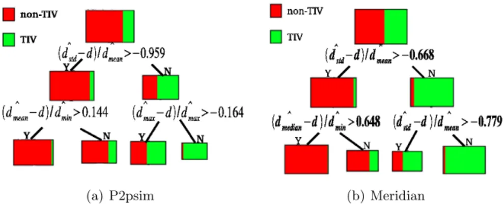
In this paper, we learned our decision trees using a data mining software called PEPITO [16] which integrates most popular machine learning algorithms. The training data collected in Section 3.1 was randomly divided into disjoint learning and test sets of roughly equal sizes. In other words, we used half of the data to build the trees and the other half to evaluate the trees. Two different trees were separately built for P2psim and Meridian, shown in Figure 24
. There are a few interesting observations to be noticed.
4
Note that the decision trees learned are essentially invariant from one simulation to another. The invariance can be extended to other results in this paper. Thus, unless otherwise stated, the results of all the experiments in the paper are derived from one simulation.
(a) P2psim (b) Meridian
Fig. 2.Top three levels of the decision trees built on P2psim and Meridian data set. The colour in the rectangular boxes reflects the proportions of TIV and Non-TIV classes.
The most discriminative variable. By examining the root nodes of both trees in Figure 2, it can be seen that the first test is on the same variable, dˆstd−d
ˆ dmean,
which appears to be the most discriminative. For the reason that will be clear in the next section, we name this variable OREE. On both trees, when the value of OREE is smaller than the cut point, the edge is more likely to be a TIV base, and vice versa. Figure 3(a) and 3(c) show the ROC5
curves of OREE, REE and std REE. Note that the ROC curve of OREE is consistently the highest while the other two variables perform inconsistently: REE is more discriminative on P2psim but less on Meridian than std REE. Figure 3(b) and 3(d) show the mean ROC curve of OREE and the covariances at some selected thresholds obtained over the 10 simulations. These figures clearly highlight that the results are very stable from one simulation to another.
The analysis of the most discriminative variable. The most discrimina-tive variable dstdˆ −d
ˆ
dmean consists of 2 parts, ˆ dstd ˆ dmean and d ˆ
dmean. The former can be
considered as a relative oscillation measure and the latter is a relative error measure. Thus, this variable is named by OREE representing Oscillation and Relative Estimation Error. Intuitively, the oscillation of the estimated distances and the embedding error are all the information one can extract and exploit for TIV detection. In fact, the ROC curves of OREE are almost identical to those of the decision trees in both networks, shown in Figure 3(a) and 3(c). This suggests that the other variables provide little extra information so that their corresponding nodes in the trees can be safely pruned with no performance degradation. Figure 4 shows the TIV and non-TIV distributions of P2psim and Meridian with respect to OREE. It can be seen that the overlap of the two
5
A ROC (Receiver Operating Characteristic) curve is a graphical plot of the true positive rates (TPR) versus the false positive rates (FPR) for a binary classifier as its discrimination threshold is varied [17].
0 0.2 0.4 0.6 0.8 1 0 0.2 0.4 0.6 0.8 1 FPR TPR Decision Tree REE Std REE OREE (a) P2psim 0 0.1 0.2 0.3 0.4 0.5 0.5 0.6 0.7 0.8 0.9 1 FPR TPR (b) 10 simulations on P2psim 0 0.2 0.4 0.6 0.8 1 0 0.2 0.4 0.6 0.8 1 FPR TPR Decision Tree REE Std REE OREE (c) Meridian 0 0.1 0.2 0.3 0.4 0.5 0.5 0.6 0.7 0.8 0.9 1 FPR TPR (d) 10 simulations on Meridian Fig. 3. ROC curves of the decision trees, obtained by varying the threshold of the probability of TIV, and of three variables including OREE, REE and std REE, ob-tained by thresholding the values of the corresponding variables. The right figures show the mean ROC curves of OREE and the covariances at some selected thresholds (the covariance ellipses are scaled by 3 times for the sake of visibility).
−50 −4 −3 −2 −1 0 1 0.02 0.04 0.06 0.08 Value of OREE Density
P2pSim TIV bases P2psim NonTIV bases
(a) P2psim −40 −3 −2 −1 0 1 2 0.01 0.02 0.03 0.04 0.05 0.06 0.07 Value of OREE Density
Meridian TIV bases Meridian NonTIV bases
(b) Meridian
Fig. 4.TIV and non-TIV distributions in P2psim and Meridian with respect to OREE. It can be seen that detecting TIVs in Meridian is much easier than in P2psim and that there is a shift between the optimal cut points for the two networks.
0 0.1 0.2 0.3 0.4 0.5 0.5 0.6 0.7 0.8 0.9 1 FPR TPR REE 2 Ticks 50 Ticks 100 Ticks (a) P2psim 0 0.1 0.2 0.3 0.4 0.5 0.5 0.6 0.7 0.8 0.9 1 FPR TPR REE 2 Ticks 50 Ticks 100 Ticks (b) Meridian
Fig. 5.ROC curves of using different numbers of ticks to compute OREE.
distributions in P2psim is much larger than in Meridian, which is the reason why the ROC curves in Meridian are much higher than those in P2psim.
How many ticks to be used. The parameter K, i.e. the number of ticks that are used to compute OREE, might affect the accuracy of our model. Figure 5 shows ROC curves obtained with different values of K. It can be seen that a noticeable improvement can be achieved even when K = 2. With a larger K, the statistical variables, mean and standard deviation, become more stable and the performance of the detection is improved. However, no or minor differences are obtained when K goes from 50 to 100, showing that the optimal value of K should probably be smaller than 100. We nevertheless set K = 100 in all our experiments since it doesn’t cause any side effect.
The variations of the decision trees. The two decision trees in Figure 2 have non-negligible variations. Even for the two root nodes that correspond to the same variable, a shift is found between the optimal cut points in them, which introduces errors when the tree learned on one network is applied to another. Table 1 shows the error rates when learning and evaluating on the same data set and on different data sets. Note that the first row specifies the data sets on which learning is carried while the first column gives the data sets on which evaluation is applied. We see that the variability of the trees indeed leads to high error rates in cross-testing. The tree learned from combining data of both networks gives better average results but is still inferior to the trees learned on each particular network. In practice, even if we can collect data and learn a specific classifier for each network, the TIV distribution in the network often evolves in time due to e.g. changes in routing or network upgrade. The next section introduces a simple but effective method for distributed TIV detection based only on OREE.
Table 1.Error rates of applying decision trees on P2psim and Meridian data sets ` ` ` `` ` `` `` ` Test Set Learning Set
P2psim Meridian P2psim+Meridian
P2psim 15.6% 43.7% 20.5%
Meridian 28.5% 8.4% 9.4%
4
Distributed TIV Detection based on OREE
We aim to embed the TIV detection algorithm into the ICS algorithm, Vivaldi in our case, so that the detection can be done at each node, i.e., each node classifies the edges with its 32 neighbors into TIV bases and non-TIV based on OREE variable.
4.1 Detection Algorithm
Recall that when the value of OREE is smaller than a cut point, the edge will be detected as TIV, and vice versa. This makes us guess that the probability of an edge being a TIV increases when the value of OREE decreases. To verify it, we sort the 32 edges connected to each node by the value of OREE in ascending order and count the number of TIV bases appearing at each position from 1 to 32. These numbers are normalized by the total number of nodes so that we have the proportion of TIVs at each position. Ideally, we would like the proportions of TIVs at one side to be close to 1 and at the other side to 0. Figure 6 shows the proportion of TIVs at each position sorted by OREE, REE and std REE respectively. 0 10 20 30 40 0 0.1 0.2 0.3 0.4 0.5 0.6 0.7 0.8 0.9 1
Different variables sorted in ascending order
Proportion of TIV REE Std REE OREE (a) P2psim 0 10 20 30 40 0 0.1 0.2 0.3 0.4 0.5 0.6 0.7 0.8 0.9 1
Different variables sorted in ascending order
Proportion of TIV
REE Std REE OREE
(b) Meridian
Fig. 6.Proportions of TIVs at each ordering position sorted respectively by OREE, REE and std REE on P2psim and Meridian data sets. It can be seen that the TIV proportions of OREE are larger on the left side and smaller on the right side, which further justifies the efficiency of OREE for TIV detection.
(a) P2psim (b) Meridian
Fig. 7.Roc curves of thresholding OREE and threshold n on P2psim and Meridian. The circles, in the upper left corner, represent the upper bounds of the detection rates by choosing an optimal, different threshold for each node.
It is clear that the proportion of TIV decreases monotonously with the order-ing position. For OREE, the probability drops below 0.5 at the 6th position for P2psim and at the 14th position for Meridian. This suggests a simple detection method that, at each node, after the 32 edges are sorted in ascending order, fixes a cut point at the nth position, where the probability of TIV at the nth position is larger than a pre-defined threshold that should be at least above 0.5.
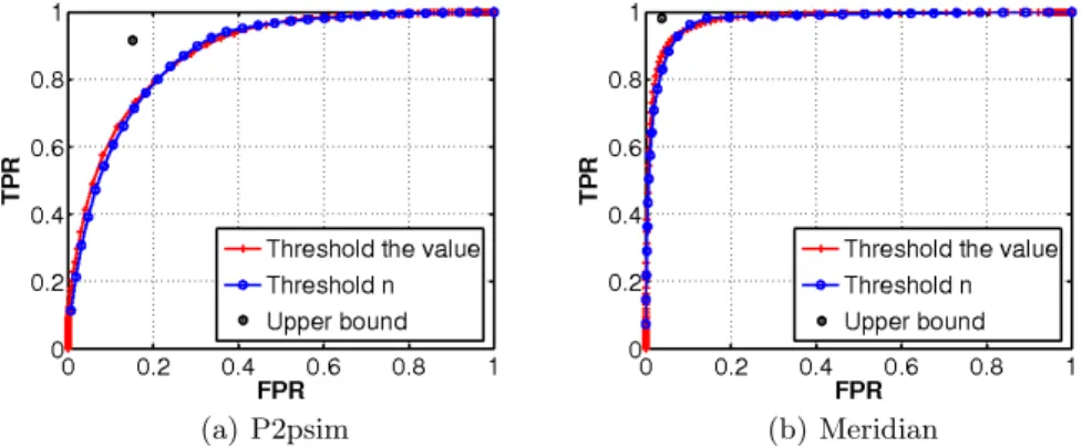
4.2 Experiments
We first compared our detection algorithm that thresholds n with an alterna-tive method that directly thresholds the value of OREE. A ROC curve can be obtained for either method by varying its threshold, shown in Figure 7. It can be seen that both methods work identically well as their ROC curves coincide, which is not surprising as the difference between them is subtle. In a distribu-tive manner, a common fixed threshold on the value of OREE is equivalent to a different threshold on n chosen at each node. On the other hand, a common fixed threshold on n for all nodes is equivalent to a different threshold on the value of OREE at each node. In a sense, these are dual methods.
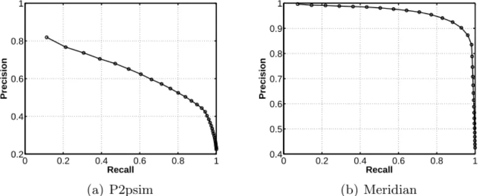
The two methods share a common problem. For decentralized detection, the optimal fixed cut point either for the value of OREE or for n can’t be found out easily. Nevertheless, the advantages of tuning n are twofold. First, n has a fixed range of [1, 32] while the value of OREE is theoretically unbounded. Then, from the ROC curves in Figure 7, it can be observed that the detection rates are influenced by n more evenly than by the value of OREE. Figure 8 shows the plot of recall versus precision by varying n. It can be seen that tuning n affects recall and precision in the opposite directions. A large n improves the recall but decreases the precision, and vice versa. In practice, the optimal n should be set to trade the precision for the recall in order to meet the specific requirements
0 0.2 0.4 0.6 0.8 1 0.2 0.4 0.6 0.8 1 Recall Precision (a) P2psim 0 0.2 0.4 0.6 0.8 1 0.4 0.5 0.6 0.7 0.8 0.9 1 Recall Precision (b) Meridian
Fig. 8.Precision versus recall of our detection algorithm by thresholding n. Precision is the ratio between the true positive and the total positive detected by the classifier, and recall is another name of true positive rate.
of different applications. For instance, when the cost that a non-TIV edge is erroneously detected as a TIV edge is large, a conservative, small n should be used, and vice versa.
Since we know whether an edge is TIV or non-TIV in the experiments, it is possible to calculate the optimal cut point at each node. To test this idea, we tried out, for each node, all possible n from 1 to 32 and recorded the particular nthat maximizes the information gain [18]. Although these optimal cut points can’t be computed in practice, they give the upper bound of the detection rates by using OREE, plotted as a circle in Figure 7, and show how much room we have to further improve our detection algorithm.
5
Conclusions and future work
This paper presents a novel approach to detecting triangle inequality violations in Internet Coordinate Systems. The strength of our approach lies in the use of supervised learning methods, particularly decision trees, that successfully find a discriminative variable for TIV detection. A simple but effective method is developed that detects TIVs at each node based on the learned variable. This allows the detection algorithm to be embedded in the ICS algorithms.
One shortcoming of the detection algorithm is that a fixed cut point needs to be set for all nodes. Clearly, the performance of detection can be further improved by choosing an optimal cut point for each node autonomously. Another limitation is that the TIV detection is treated as a classification problem that classifies edges between nodes as TIV or non-TIV. In practice, it would be more useful to reason on the severity of the violations, which is a continuous value instead of a discrete level. This requires to solve a regression problem, which is expected to be more difficult than the classification problem addressed in this paper.
References
1. Azureus Bittorrent. http://azureus.sourceforge.net.
2. Ratnasamy, S., Handley, M., Karp, R., Shenker, S.: Topologically-aware overlay construction and server selection. In: Proc. IEEE INFOCOM, New York, NY, USA (June 2002)
3. Zhang, R., Tang, C., Hu, Y.C., Fahmy, S., Lin, X.: Impact of the inaccuracy of distance prediction algorithms on internet applications: an analytical and compar-ative study. In: Proc. IEEE INFOCOM, Barcelona, Spain (April 2006)
4. Ng, T.S.E., Zhang, H.: A network positioning system for the internet. In: Proc. of USENIX Annual Technical Conference. (June 2004)
5. Dabek, F., Cox, R., Kaashoek, F., Morris, R.: Vivaldi: A decentralized network coordinate system. In: Proc. ACM SIGCOMM, Portland, OR, USA (August 2004) 6. Costa, M., Castro, M., Rowstron, R., Key, P.: Pic: practical internet coordinates
for distance estimation. In: Proc. the ICDCS. (2004) 178–187
7. Zheng, H., Lua, E.K., Pias, M., Griffin, T.: Internet Routing Policies and Round-Trip-Times. In: Proc. the PAM Conference, Boston, MA, USA (April 2005) 8. Lee, S., Zhang, Z., Sahu, S., Saha, D.: On suitability of euclidean embedding of
internet hosts. SIGMETRICS 34(1) (2006) 157–168
9. Kaafar, M.A., Gueye, B., Cantin, F., Leduc, G., Mathy, L.: Towards a two-tier internet coordinate system to mitigate the impact of triangle inequality violations. In: Proc. IFIP Networking Conference. LNCS 4982, Singapore (May 2008) 397–408 10. Kaafar, M.A., Cantin, F., Gueye, B., Leduc, G.: Detecting triangle inequality violations for internet coordinate systems. In: Proc. International Workshop on the Network of the Future, Dresden, Germany (June 2009)
11. Wang, G., Zhang, B., Ng, T.S.E.: Towards network triangle inequality violation aware distributed systems. In: Proc. the ACM/IMC Conference, San Diego, CA, USA (oct 2007) 175–188
12. Littman, M.L., Ravi, N., Fenson, E., Howard, R.: Reinforcement learning for auto-nomic network repair. In: 1st International Conference on Autoauto-nomic Computing (ICAC). (2004)
13. Khayat, I.E., Geurts, P., Leduc, G.: Machine-learnt versus analytical models of TCP throughput. Computer Networks 51(10) (July 2007) 2631–2644
14. A simulator for peer-to-peer protocols. http://www.pdos.lcs.mit.edu/p2psim/ index.html.
15. Wong, B., Slivkins, A., Sirer, E.: Meridian: A lightweight network location service without virtual coordinates. In: Proc. the ACM SIGCOMM. (aug 2005)
16. PEPITO: A data mining software. http://www.pepite.be.
17. Fawcett, T.: Roc graphs: Notes and practical considerations for researchers. Tech-nical report, HP Laboratories (March 2004)
18. Breiman, L., Friedman, J.H., Olshen, R.A., Stone, C.J.: Classification and Regres-sion Trees. Wadsworth International, California (1984)