Considering the effects of localised fires in the numerical analysis of a
building structure
Jean-Marc Franssen, Dan Pintea, Jean-Claude Dotreppe Univ de Liège, 1 Chemin des Chevrevils, 4000 Liège, Belgium Abstract
The methodologies that are used for analysing the fire behaviour of a structure that is subjected to a uniform thermal situation cannot be applied when the fire is localised. The concept of "zoning" can be applied: the structure is divided into several zones in which the situation is approximated as uniform. It is shown here that this division can lead to spurious forces in the structure. The structural code of the first author has been adapted in order to accommodate a continuous spatial variation of the fire environment. A series of uncoupled 2D thermal analyses is performed along the length of the beam finite elements and a series of ID thermal analyses is performed across the thickness of the shell finite elements. After a discussion of the concept and the
particularities dictated by the continuous thermal environment, the methodology utilised is explained and is shown in an example consisting of a composite steel concrete car park subjected to a localised fire of the type given in Eurocode 1.
Keywords: Localised fire; Fire resistance; Numerical model Nomenclature
Am surface area of a member per unit length
C specific heat
Li interface length
V volume of a member per unit length u longitudinal displacement
x distance along the abscise ε strain εm mechanical strain εth thermal strain λ thermal conductivity ρ specific mass 1. Introduction
When structural elements are tested against fire in a furnace, every precaution is taken in order to have a uniform spatial distribution of the temperature in the furnace or, more precisely, to have a uniform thermal attack on the elements. In real buildings, the fully developed fire that usually takes place in the compartment is considered to be represented accurately enough by a one-zone situation, which means that the conditions in terms of gas temperatures or incident heat flux to the structure are uniform.
This uniform situation has direct consequences on the numerical simulations that are performed to model the behaviour of the structure. The temperature distribution in the flat elements such as walls, floors and ceilings is essentially one-dimensional (1D), with a gradient only across the thickness of the slab. In linear elements, such as beams and columns, the temperature distribution is essentially two-dimensional (2D) with no variation along the length of the elements. This particular temperature distribution is of course taken into account in the analyses and, in beams for example, as long as the cross-section remains the same, the same temperature distribution is considered for every longitudinal point of integration. The same holds in the slabs for every point of integration in the plane of the elements. The temperature distribution can have a 2D (for slabs) or three-dimensional (3D) (for beams) pattern near the edges of the compartment because of the influence of the adjacent cold
compartments, but this effect is strongly localised and is usually neglected.
There are yet some situations when the thermal attack from the fire is inherently variable in space. This is in fact the case, with very few exceptions, at the beginning of every fire; any fire is localised in the compartment before it turns into a fully developed fire. This preliminary phase is usually disregarded for the analysis of the structural
behaviour because the low temperatures associated to this phase are considered to have negligible effects on the structure. In some cases, even this localised fire may be a threat for the structure. One example is a localised fire under a statically determinate steel truss girder: losing the one member of the truss that is located just above the fire leads to the loss of the whole girder.
Some fires keep a localised character during the entire duration. This can be the case if the fire area is localised within the compartment, for example, if a ticket counter is the only engulfed area in an otherwise much larger entrance hall of a railway station or if a few cars burn in a large car park. In these cases, even if the structure is statically indeterminate, a proper analysis of the structural behaviour must take into account the spatial variability of the thermal boundary conditions.
This paper discusses some of the aspects related to this spatial variability and gives some indications how they can be incorporated into a numerical analysis in a cost-effective way. Two points are essentially discussed: the 3D character of the temperature distribution and the proper consideration of the temperature distribution in the finite elements.
2. Thermal problem
If the thermal boundary conditions vary along the two planar coordinates of a slab and if the slab is thermally thick enough to create thermal gradients across the thickness of the slab, which is the case except in very thin steel sheets, then the temperature distribution shows a 3D pattern in the slab. If the thermal boundary conditions vary along the longitudinal coordinate of a beam and if the cross-section of the beam is thermally thick enough to create thermal gradients in the section, which is the case except in very thin steel bars, then the temperature distribution shows a 3D pattern in the beam.
Does it mean that this 3D temperature distribution has to be explicitly taken into account and that it can be determined only by a full 3D thermal analysis? If this is the case, the cost in term of time required to build the model, in terms of memory allocation and in terms of computing time would be prohibitive for any structure of a significant size. Two different aspects of the question have to be considered: the variability of the temperature at the joints between adjacent structural members and the variability of the temperature along each member.
2.1. Variability at the joints
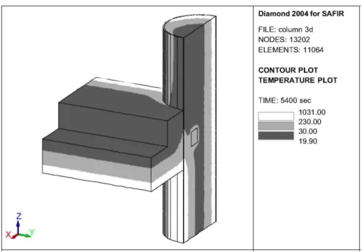
A joint between adjacent beam-type members is a geometrically complex object, especially if more than two members meet at the joint and these members are of different sizes. Flush end plates, stiffeners, angles, bolts or welds and gaps of different sizes are commonly present in these joints and they all influence the temperature distribution and the heat flow from one member to the other. The exact representation of the thermal situation in the joint can only be made by means of a multitude of 3D finite elements for each joint. Such analyses have been done in the past, usually with the aim of analysing the temperature distribution in detail in a single joint, without any subsequent structural analysis being made on the model. In these thermal analyses, the thermal boundary conditions are either uniform, or they vary in a discrete manner from one to the other side of the joint. For example, the part of a column that is located below the joint is submitted to the fire whereas the part of the column that is located above the joint is in a room-temperature environment. Even in these cases of stepwise variation of the boundary conditions, it has been observed that the perturbation of the 2D temperature
distribution that prevails in the members away from the joint is limited to a short distance from the joint, see Fig. 1. This means that it can be considered as an acceptable simplification to perform the 3D thermal analysis of each beam member separately, neglecting the local influence of the joint.
It has to be mentioned that the subsequent structural analysis that will be made of the structure normally relies on oriented finite elements such as beam elements because a structural analysis of a complete building based on 3D solid elements is unfeasible. These oriented elements do not have the capability to take into account the real 3D stress distribution that prevails in the joints. Some simplifications are also made near the joints when using these elements. In other words, the richness of a full 3D temperature distribution that could eventually be calculated in the joints cannot be exploited by the oriented elements used in the structural analysis.
Thus, instead of a full 3D thermal analysis of the complete structure, it is acceptable to perform a series of 3D thermal analyses, each one in a defined structural member, a slab, a wall, a beam, a column or a member in a truss, neglecting the heat flux and the associated temperature perturbation created by the joints. This reduces the unfeasible problem into a series of problems of reasonable size.
2.2. Variability along the members
The question examined here is how a variation of the boundary conditions along the axis of a member is reflected in the temperature distribution. In order to investigate this question, a steel member has been analysed because steel has a higher thermal conductivity than concrete and is the material that will have the highest capability to transmit a heat flux along the elements.
Fig. 1. Isotherms in a joint between a composite column and a concrete slab after 90min of IS0834 fire exposure
(value of the isotherms in °C).
The most severe variation of the boundary condition that could exist is a stepwise variation, quite unlikely to occur in reality. The situation considered here is an incident flux of 100 kW/m2 on one part of a steel member and a sudden drop to zero for the other part of the member. This value of 100 kW/m2 has been chosen because it is the highest possible incident flux according to Annex C of Eurocode 1 [1]. A boundary with air at 20°C is imposed on the entire length of the plate, for simulating the environment to which the structure reradiates. The temperature variation along the length of the plate will be examined.
The temperature on the cross-section of a steel member is quite uniform. The problem has been analysed as a 2D situation as would be relevant, for example, for a plate (web or flange) of a steel profile; one dimension is the longitudinal axis of the steel member and the other dimension is across the thickness of the plate, see Fig. 2. Four values of the section factors Am/V have been analysed, namely 40, 80, 250 and 400 m-1, corresponding to
plate thicknesses of 50, 25, 8 and 5 mm, with the fire applied on both sides (1/2 of the thickness considered in the analyses owing to symmetry).
Each plate has been analysed without protection and then with thermal protection on each face (20 mm of a hypothetical product with λ = 0.08 W/mK and cρ = 170kJ/km3 (no water content)). Thermal properties of steel and boundary conditions are from Eurocode 3 [2].
A 100-mm-thick concrete slab has also been submitted to the same discontinuous boundary conditions.
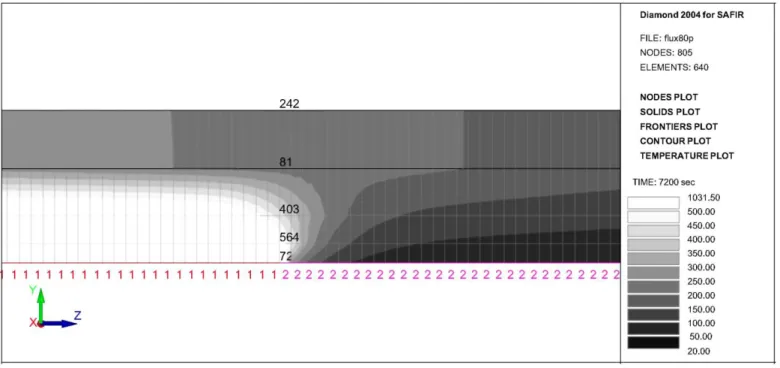
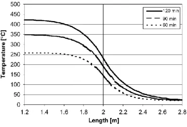
The results can be seen in terms of isotherms at a given time, see, for example, Fig. 3 for a protected steel plate, or in terms of temperature evolution along the plate at various times, see Fig. 4.
The results of all calculations are summarised in Table 1 in which the interface length Li is defined as the
distance:
• from the point where the boundary conditions change (see Point A in Fig. 2, or line from node 72 to node 242 in Fig. 3,or the point at abscise x = 2m in Fig. 4);
• to the point along the plate where the steel temperature changes by less than 10 °C to the left (Hot zone) and to the right (Cold zone) compared to the values at the end of the plate, where the perturbation has no influence. For the concrete slab, the interface length is evaluated on the exposed surface.
It can be observed that the interface length:
• is longer in protected sections than in unprotected sections, • is longer in massive sections than in thin sections,
• increases with time but tends towards a constant value (because the problem tends towards a steady-state situation),
• is longer in the cold part than in the heated part, and
• is significantly smaller in the concrete slab than in steel plates.
Fig. 2. Steel bars with a stepwise variation of the boundary conditions.
Fig. 3. Isotherms after 2h of IS0834 fire applied on the left part of a protected 80mm steel plate (values in °C).
In all situations, the interface length is rather limited; not more than twice the thickness in the concrete slab and not more than 0.5 m in the steel members. These values have been obtained with a variation in the boundary conditions that is quite extreme and unrealistic. It can be inferred from this analysis that if the temperature in the bars or in the slabs has a tendency to go back to the undisturbed values at a rather short distance of the
perturbation when this perturbation is so severe, then this would be the case for even much shorter distances if the perturbation is less severe, for example, in the case of a continuous variation of the boundary conditions along the length of the member.
It has indeed been observed [3] that in a IPE600 steel beam submitted to the highly localised fire model of Eurocode 1, the temperature in the sections is very similar when it is calculated either as a series of 2D
calculations in different sections, that is without any consideration for the longitudinal heat flows, or as a single 3D calculation in the complete beam.
Fig. 4. Evolution of the temperature along the protected 80 mm plate for the IS0834 fire applied on the left-hand
side (up to 2 m).
Table 1: Interface length Li in various situations
t (mm) Protection Time (min) Li (mm)
Hot zone Cold zone
40 No 10 158 215 40 No 20 165 336 40 No 30 221 429 25 No 10 108 237 25 No 20 156 357 25 No 30 143 444 8 No 10 78 259 8 No 20 71 354 8 No 30 70 411 5 No 10 57 256 5 No 20 56 331 5 No 30 56 364 40 Yes 60 293 328 40 Yes 90 405 463 40 Yes 120 497 580 25 Yes 60 345 400 25 Yes 90 445 539 25 Yes 120 522 655 8 Yes 60 352 466 8 Yes 90 406 585 8 Yes 120 393 674 5 Yes 60 322 464 5 Yes 90 266 563 5 Yes 120 405 633 Concrete No 60 41 119 Concrete No 90 46 152 Concrete No 120 49 178
2.3. Conclusion
As a conclusion of the above discussion, it seems to be a sufficiently good approximation to calculate the temperatures in a structure subjected to a localised fire as a series of uncoupled 1D calculations in the slabs and walls, and as a series of uncoupled 2D calculations in beams and columns. The effect of the variation of the longitudinal boundary conditions that is not considered is negligible on the temperatures. The effect at the joint between adjacent members is more significant but a structural analysis based on oriented members such as beam or shell finite elements is anyway not capable of taking the true temperature field in the joints into account. 3. Structural problem
The question examined here is the influence that the degree of precision in the representation of the temperature distribution has on the stress distribution in finite elements. Only the influence of a longitudinal variation of temperature will be examined here because this is the typical consequence of a localised fire. The question is examined separately for the beam and for the shell finite elements.
3.1. In beam finite elements
If the temperature is varying along the length of an otherwise unstressed beam, this temperature variation should not generate any stress in the beam. What kind of representation of the temperature variation has to be taken into account for not generating spurious stresses in beam finite elements?
If the average temperature along the length of the element is taken into account, the thermal strain εth is a
constant. If the longitudinal field of displacement u(x) is a linear function of the longitudinal coordinate x (which is typical in elements with 2 nodes), then the strain is also a constant and the element can find a position, in fact a thermal elongation, leading to no mechanical strains and hence to no stresses. If a linear variation of the temperature along the length is taken into account, the thermal strain is a linear function of x.
• If the longitudinal field of displacement u(x) is linear, then the strain is a constant and the mechanical strain will be linear whatever the thermal elongation of the member because The element will share the thermal elongation between the longitudinal points of integrations, creating spurious compression stresses in some points and spurious tensile stresses in others.
• If the longitudinal field of displacement u(x2) is a second-order function of x, then the strain
is linear the element can find a position leading to no mechanical strains and hence to no stresses. The software SAFIR [4], for example, has a non-linear longitudinal displacement field owing to a 3rd central node that bears the nonlinear component of the longitudinal displacement. It is thus capable of
representing linear temperature distributions whereas most common elements with only 2 nodes are not. Fig. 5 shows the diagram of axial force in a hypothetical 10 m long cantilever beam subjected to a localised fire located 2.5 m under the supports (on the left of the figure). The beam finite element has been forced to be linear in this application. After 1 m, the uniform temperature in element 2, for example, is 488 °C at the first
longitudinal point of integration and 276 °C at the second point of integration. The axial force at these integration points is +82 and -82 kN which, for this IPE80 section, leads to spurious stresses of 107N/mm2. When the longitudinal displacement in the elements is allowed to be a second-order function of the longitudinal coordinate, the axial force at the same instant drops to <10-4N.
3.2. In shell finite elements
If a localised fire is circular in shape (plan view), the thermal gradients in the plane of a horizontal slab situated above the fire are radial around the point where the fire impinges on the slab. If the thermal gradient in the radial direction is linear and there is no gradient in the circumferential direction, a shell finite element in which the membrane displacement is a linear function of the two planar coordinates will generate spurious stress in the radial direction, but none in the circumferential direction. A finite element in which the membrane displacement field is a second-order power of the planar coordinates is required to represent the linear thermal gradient without any spurious stresses.
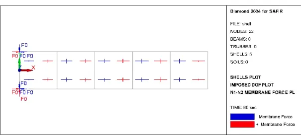
If the shell element is linear, the spurious radial stresses cannot be avoided and their influence must be evaluated. Fig. 6 shows the membrane forces in a hypothetical 5-m-long cantilever beam made of a 1000-mm-wide 20-mm-thick steel plate in which a thermal gradient of -100°C/m has been introduced in the X direction. This cantilever beam is here modelled by 5 linear shell finite elements. It can be observed that the most important spurious stresses are in the direction of thermal gradient (in the order of 85N/mm2), with smaller stresses also observed in the transverse direction (in the order of 30 N/mm2).
Fig. 5. Axial force diagram in a linear beam element (localised fire under the left-hand side of the beam).
Fig. 6. Membrane forces in a steel plate with linear thermal gradient in the X direction.
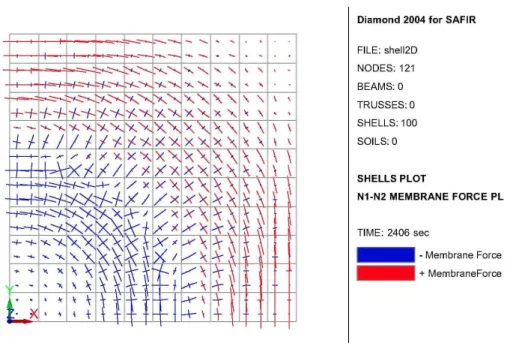
Fig. 7 shows the distribution of membrane forces in a steel plate subjected to a localised fire in the centre (1/4 only represented owing to symmetry). Although the theoretical solution to this problem is not available (all material properties are non-linear), the stress distribution fits with common sense and is quite continuous, which seems to be an indication that spurious stresses are of a lower order of magnitude than the true stresses. This application seems to indicate that, on the contrary to what is indicated by Fig. 6, the results produced by a linear shell element may be a good approximation of the "correct" results.
4. Algorithmic modifications
When the thermal calculation is performed under the hypothesis of uniform boundary conditions, the position of the structural element under consideration with respect to the fire does not need to be known. It is standard practice to perform the thermal analysis first, without any consideration of the real position of the structure that will be considered subsequently in the mechanical analysis. When the fire is localised, the boundary conditions
for the thermal analysis are highly dependent on the location of the relevant element with respect to the fire in the compartment; virtually every element has a different position. For this position to be known requires that the structural model has been defined before the thermal calculations are performed. Either the thermal model must have access to the file in which the structure is defined in order to determine automatically the position of the analysed element in the structure, or the user has to provide the information himself for each thermal analysis. If the size of the section considered is small with respect to the size of the compartment, it may be sufficient to represent the position of the section by the position of one characteristic point, its centre of gravity for example. Various algorithmic modifications may be required when the localised nature of the fire is considered because the temperature distribution in the beams, for example, is no longer the same in all sections (the same holds for shells). Much more information has to be stored in the data file.
Fig. 7. Membrane forces in one-fourth of a steel plate with radial thermal gradient.
5. Application
An example is presented here as an application of the previous concepts and as a validation of the algorithmic modifications. In order to eliminate the complexity of the problems linked to the CFD software that can be used to determine the thermal situation in the compartment, the localised fire is taken according to the localised model presented in Annex C of Eurocode 1 [1].
The structure is part of composite deck steel frame building used as an open car park, see Fig. 8. In the X direction, the 15cm slab has 7 spans of 5.4m, i.e., a total length of 37.8 m. In the Y direction, the columns are spaced at 15 m, which makes a total length of 30 m. The external columns are made of HE300AA, the central columns are made of HE500A and the beams of IPE500 sections. The beams extend only in the Y direction. The concrete slab is linked to the steel beams, which generates a composite behaviour. The figure shows different colours in the shells because the reinforcing bars are different in the spans and on the supports.
The fire source is created by four cars located side by side at Y =27 m, with the first car burning at X = 18.9, i.e., in the centre of span 3. Cars 2, 3 and 4 are at X = 21.6, 24.3 and 27 m, respectively. There is a delay of 12min for the fire to propagate from each car to the next one, with car 1 being the first ignited. The maximum heat release rate for each car (9.8 MW) is reached 30 min after it ignites.
Approximately one-third of the car park is supposed to be affected by the fire, whereas the rest is supposed to remain at room temperature.
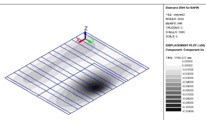
Fig. 9 shows the vertical displacements in the slab after 20 min of fire. At this moment, cars 1 and 2 are on fire. The displacement pattern is continuous but this is inherent to the formulation of these displacement-based elements. It would also be the case even if significant spurious stresses were present.
Fig. 10 is more interesting because it shows how the bending moments are distributed continuously,
notwithstanding the local character of the fire and the rather high aspect ratio (1:3.4) for some shell elements. This example seems to indicate that, in this case, the spurious stresses inherent to the linear shell elements are negligible compared to the true stresses.
Fig. 10. Bending moments after 20 min of localised fire.
6. Conclusions
The basic concepts for considering a localised fire into a numerical structural model have been highlighted. The link that exists between, on the one hand, the hypotheses made for the variation of the temperatures and of the displacements in the elements and, on the other hand, the stresses that are evaluated, has been discussed. The applicability of these concepts has been shown for a particular case in which the localised fire is based on Annex C of Eurocode 1. The route has thus been paved for analysing a structure for which the thermal environment would be determined by CFD software.
References
[1] Eurocode 1. Actions on structures—part 1—2, general actions— actions on structures exposed to fire. EN 1991-1-2. CEN; Brussels: CEN; November 2002.
[2] Eurocode 3. Design of steel structures—part 1—2, general rules—structural fire design. ENV 1993-1-2. Brussels: CEN; 1995. [3] Gens F, Franssen J-M & Dotreppe J-C, Effect of localised fires on continuous steel beams, EUROSTEEL 2005. In: Hoffmeister B., Hechler O., editors., Proceedings of the fourth European conference on steel and composite structures, Aachen, 2005. p. 85-92. [4] Franssen J-M. SAFIR, A thermal/structural program modelling structures under fire. Eng J AISC 2005;42(3): 143-58.