! "!
Concurrent observations of the ultraviolet nitric oxide
and infrared O
2nightglow emissions with Venus Express
J.-C. Gérard, C. Cox, L. Soret, A. Saglam Laboratoire de Physique Atmosphérique et Planétaire
Université de Liège, Belgium
G. Piccioni IASF-INAF, Roma, Italy
J.-L. Bertaux
Service d'Aéronomie du CNRS, Verrières-le-Buisson, France and
Institut Pierre Simon Laplace, Université de Versailles-Saint-Quentin, France
P. Drossart
LESIA, Observatoire de Paris, Meudon, France
Accepted for publication in J. Geophys. Res. Final, May 2009
! "! Abstract
#! "!
Two prominent features of the Venus nightside airglow are the nitric oxide ! and " bands $!
produced by radiative association of O and N atoms in the lower thermosphere and the O2
%!
infrared emission generated by three-body recombination of oxygen atoms in the upper &!
mesosphere. The O2 airglow has been observed from the ground, during the Cassini flyby and
'!
with VIRTIS on board Venus Express. It now appears that the global structure of the two (!
emissions shows some similarities, but the statistical location of the region of strongest )!
emission are not coincident. The SPICAV ultraviolet spectrograph has collected a large *!
number of spectra of the Venus nitric oxide nightside airglow. VIRTIS spectral images have #+!
been obtained at the limb and in the nadir-viewing mode and have provided new information ##!
on the horizontal and vertical distribution of the emission. We present the first concurrent #"!
observations of the two emissions observed with Venus Express. We show that nadir #$!
observations generally indicate a low degree of correlation between the two emissions #%!
observed quasi-simultaneously at a common location. A statistical study of limb profiles #&!
indicates that the altitude and the brightness of the two airglow layers generally do not co-#'!
vary. We suggest that this lack of correlation is explained by the presence of strong horizontal #(!
winds in the mesosphere-thermosphere transition region. They carry the downflowing atoms #)!
over large distances in such a way that regions of enhanced NO emission generally do not #*!
coincide with zones of bright O2 airglow.
"+! "#!
! $! "#!
I. INTRODUCTION
""!
Planetary airglow is a powerful way to remotely probe the characteristics of "$!
atmospheres from an orbiting or flying-by spacecraft that complement in situ measurements. "%!
In particular, the study of airglow morphology, time variations and brightness may provide "&!
key observations concerning atmospheric composition, temperature structure, transport "'!
processes and their response to the solar photon and particle inputs. In the case of Venus, the "(!
Venera and Pioneer Venus missions have shed new light on some of these aspects more than ")!
twenty-five years ago. The presence of the delta and gamma bands of nitric oxide in the "*!
Venus nightglow was detected and identified by Feldman et al. [1979] using the ultraviolet $+!
spectrograph on board the International Ultraviolet Explorer (IUE). It was also observed by $#!
Stewart and Barth [1979] with the ultraviolet spectrometer on board the Pioneer Venus
$"!
Orbiter (PV-OUVS). The emission is produced by radiative recombination through inverse $$!
predissociation of nitrogen N(4S) and oxygen O(3P) atoms and dominates the middle $%!
ultraviolet nightglow spectrum. In this process, excited NO molecules radiate the ultraviolet ! $&!
and " bands between 180 and 310 nm: $'!
N + O # NO (C 2
$) $(!
giving rise to: $)! NO (C 2$) # NO (X 2$) + !-bands $*! and %+! NO (A 2%, v’=0) # NO (X 2$) + "-bands %#!
Emission from the C 2
$ (v=0) ! A 2% (v=0) transition at 1.224 µm which populates the A 2% %"!
(v=0) level was recently observed with VIRTIS-M in the Venus nightglow [Garcia Muñoz et %$!
! %!
al., 2009]. The N and O atoms are mainly produced by dissociation of N2 and CO2 on the
%%!
dayside by extreme ultraviolet (EUV) photons and photoelectrons. %&!
Stewart et al. [1980] obtained images of the Venus nightside in the ! (0,1) band at 198
%'!
nm every 24 hours with PV-OUVS when Pioneer-Venus was near apoapsis. They showed %(!
that the emission was highly variable in brightness and morphology over consecutive 24-%)!
hours periods. The location of the brightest spots ranged from 2130 to 0300 LT and 39° S to %*!
60°N [Bougher et al., 1990]. This variability appeared to be caused by instabilities in the &+!
large-scale circulation, possibly as a result of wind shears near the terminator or time-varying &#!
wave drag from gravity waves. Stewart et al. [1980] built up a global map of the UV &"!
nightglow showing that the emission is concentrated in a bright spot located near 0200 local &$!
solar time, south of the equator. Bougher et al. [1990] estimated the emission rate of this &%!
enhanced emission to be ~1.9 kilo-Rayleighs (kR) whereas the average hemispheric nightside &&!
intensity is 0.48 kR. These observations confirmed the general picture where production of O &'!
and N atoms by solar EUV on the dayside is followed by global circulation to the nightside, &(!
downward transport and radiative recombination. The shift of the statistical bright spot toward &)!
dawn was interpreted as a signature of a residual super-rotation into the lower thermosphere. &*!
A determination of the altitude of the emission peak byGérard et al. [1981] concluded that
'+!
the emission peak is located close to 115 km. Using a one dimensional model, they derived an '#!
eddy diffusion coefficient K~8x10¹²/n1/2 cm2 s-1, where n is the total number density. The
'"!
general picture of production of O and N atoms followed by transport to the nightside by the '$!
subsolar to antisolar circulation, downward turbulent mixing and radiative recombination '%!
appeared quantitatively consistent with the PV-OUVS observations. This concept was '&!
numerically validated by three-dimensional simulations using the Venus Thermospheric ''!
General Circulation Model (VTGCM) [Bougher et al., 1990]. The statistical location of the '(!
bright spot was reasonably well predicted by the three-dimensional model and implied zonal ')!
! &! winds of about 50-75 m s-1 in the 115-150 km region. The observed shift toward dawn of the '*!
statistical location of the airglow maximum was reproduced by the VTGCM. (+!
Limb observations of the spectrum of nightglow emission in the ! and " bands of NO (#!
with the SPICAV ultraviolet spectrometer on board Venus Express [Titov et al., 2006; ("!
Svedhem et al., 2007] have been recently reported by Gérard et al. [2008a]. The mean altitude
($!
of the emission layer was found to be located at 113 km, with variations between 95 and 132 (%!
km. The mean limb brightness of the total NO emission at the limb was 32 kR, but it is highly (&!
variable with limb intensities as large as 440 kR and values below 5 kR at northern mid-('!
latitudes. It was found that the mean altitude of the emission peak statistically drops with ((!
increasing latitude between 6° and 72° N. From model fits to observed profiles, they ()!
determined that the downward flux of N atoms at 130 km typically varies between 1x10⁸ to (*!
4x10⁹ atoms cm-2 s-1. The eddy diffusion coefficient K deduced from comparisons to the )+!
observed limb profiles was significantly less than that determined from the observations made )#!
with the Pioneer Venus UV spectrometer at low latitudes during periods of high solar activity. )"!
The oxygen airglow (0-0) emission at 1.27 µm is the most intense non-thermal )$!
component in the Venus atmosphere. It belongs to the a1&g – X 3%g Atmospheric Infrared
)%!
system and corresponds to an electric dipole forbidden transition with a radiative lifetime of )&!
about 70 min. [Miller et al., 2001]. It was first discovered in ground-based observations of )'!
Venus by Connes et al. [1979] and subsequently imaged with ground-based telescopes [Allen )(!
et al., 1992; Crisp et al., 1996; Lellouch et al., 1997; Ohtsuki et al., 2008; Bailey et al., 2008].
))!
It was measured from space during the Cassini flyby with a local maximum brightness of )*!
about 4 MR [Drossart et al., 1993]. The oxygen IR nightglow appeared patchy, highly *+!
variable with asymmetries, often exhibiting multiple local maxima, with variations on *#!
timescales as short as 1 hour. A much weaker O2 airglow was also detected in the Herzberg II
*"!
visible wavelengths [Krasnopolsky et al., 1986; Bougher and Borucki, 1994]. The 1.27 µm *$!
! '! emission is produced by recombination of oxygen atoms created by photodissociation of CO2
*%!
and CO at thermospheric altitudes on the dayside. As previously explained, O atoms are *&!
transported to the nightside by the global thermospheric circulation. Three-body *'!
recombination of O atoms in the upper nightside mesosphere (95–110 km) leads to O2
*(!
formation in excited states, followed by airglow emissions as the molecules relax to the X 3%g
*)! ground state: **! #++! O + O + M ! O2* + M #+#! followed by #+"! O2* ! O2 + h' #+$! #+%!
where O2* indicates one of the excited states of the O2 molecule and M is any neutral #+&!
constituent. A fraction of the O2 molecules, estimated to be about 7%, is formed directly in #+'!
the a1&g metastable state. A substantial fraction of the upper excited states cascades into the #+(!
1
& state, so that the net efficiency of the production of this state in the three-body
#+)!
recombination may be close to 100% [Crisp et al., 1996]. Below the emission peak, O2 1&g #+*!
molecules may be deactivated by collisions with CO2, causing non-radiative transitions to the ##+!
O2 ground state. The altitude of the peak of the 1.27 µm emission is thus controlled by the ###!
competition between vertical transport, recombination and quenching. The emission rate is
##"!
related to the downward flux of oxygen atoms.
##$!
The VIRTIS-M O2 airglow limb observations have been presented by Drossart et al. ##%!
[2007a], Gérard et al. [2008b, 2009] and Piccioni et al. [2009a]. Drossart et al. [2007a]
##&!
determined that the O2 peak emission is located near 96 km, which is consistent with three-##'!
body recombination of oxygen atoms. Gérard et al. [2008b] found that limb profiles observed
##(!
at northern mid-latitudes exhibit large intensity variations over short time periods. Gérard et
! (!
al. [2009] described further emission limb profiles extracted from the images. They
##*!
determined the vertical distribution of O2 (1&g) atoms using an Abel inversion of the radiance #"+!
limb profiles. Assuming photochemical equilibrium for O2 (1&), they used these density #"#!
profiles combined with the CO2 vertical distribution to determine the atomic oxygen density. #""!
Piccioni et al. [2009a] analyzed limb measurements from 42 orbits. They found that the peak
#"$!
altitude of the O2 (1&g) volume emission rate is typically located between 95 and 100 km, with #"%!
a mean value of 97.4 ± 2.5 km. The vertical profile is broader near the equator, with a full
#"&!
width at half maximum of 11 km, a factor 2 larger than at middle latitudes. They reported that
#"'!
a secondary peak is frequently observed between 103 and 105 km.
#"(!
VIRTIS night-side observations from Venus Express have complemented
ground-#")!
based observations at much higher spatial resolution. In addition, limb observations from an
#"*!
orbit around Venus have given unprecedented access to the vertical distribution of the airglow
#$+!
layer and provided key constraints on the models. Drossart et al. [2007a] confirmed that the
#$#!
O2 nightglow exhibits a large spatial and temporal variability. Observations by VIRTIS in the #$"!
nadir mode have been used to construct extensive maps of the Venus atmosphere in the O2 #$$!
emission band [Gérard et al., 2008b, Piccioni et al., 2009a]. In nadir viewing geometry, the
#$%!
contamination of the O2 airglow by the thermal emission of the deeper atmosphere has to be #$&!
subtracted to obtain clean O2 airglow images. The mean value, integrated over the nightside #$'!
of the southern hemisphere, is typically about 0.8 MR, which is in agreement with the early
#$(!
ground-based observations giving a mean brightness of 1.2 MR for the night side. Hueso et
#$)!
al. [2008] found that the airglow is highly inhomogeneous with the regions of highest
#$*!
intensity generally located at low latitudes near the midnight meridian. They showed that
#%+!
zonal velocity derived from the motion of airglow features is dominated by an intense
#%#!
prograde jet from dawn to midnight extending up to 22 hours in local time, with lower
#%"!
velocities and reversed sign from dusk. The brightest small-scale ((100 km) features appeared
! )!
correlated with locations of apparent convergence which may be a signature of compression
#%%!
and downwelling. Piccioni et al. [2009a] described the characteristics of the horizontal
#%&!
distribution of the airglow and showed that regions of high O2 airglow intensity are associated #%'!
with downwelling causing an increase of the infrared brightness temperature. A similar
#%(!
conclusion was reached by Bailey et al. [2008] who derived rotational temperatures in excess
#%)!
of the VIRA values in regions of enhanced O2 1& emission rate. He associated these regions #%*!
with conditions of larger downflow velocities where local temperature is increased by
#&+!
compressional heating. Similar and larger temperature enhancements were observed with
#&#!
SPICAV from measurements of UV CO2 absorption measurements during stellar occultations #&"!
by Bertaux et al. [2007].
#&$!
The non-homogeneous, time-dependent distribution of the O2 1&g nightglow indicates #&%!
that the local downward flow of oxygen may differ substantially from the mean value, in
#&&!
response to variations in the efficiency of the global day-to-night transport, the focusing effect
#&'!
of the night-side subsidence, changing zonal wind speeds, eddy transport efficiency, and
#&(!
gravity wave breaking.
#&)!
The NO and O2 nightglows do not occur at the same altitude and thus provide #&*!
information about different vertical levels: 95–105 km for O2 airglow (Piccioni et al., 2009a)
#'+!
and ~115 km for NO [Gérard et al., 2008a]. In this study, we address the question of the co-#'#!
variation of the two airglow layers. Earlier studies have established that the statistical location #'"!
of the nightglow bright spots is not coincident. This result was unexpected since the two #'$!
emissions are produced by recombination of atoms created on the dayside by #'%!
photodissociation and transported to the nightside by the subsolar to antisolar global #'&!
circulation. In this study, we take advantage of the unique opportunity offered by two #''!
instruments of the Venus Express mission (SPICAV and VIRTIS) to observe almost #'(!
simultaneously the two emissions and to investigate if their characteristics co-vary in time and #')!
! *! space. The observations reported here were obtained both in nadir-viewing geometry, where #'*!
horizontal variations of the emission rate can be mapped, and at the limb, where vertical #(+!
variations are best investigated. We describe both types of observations and draw conclusions #(#!
on the level of covariance we have observed and transport processes occurring in the Venus #("!
mesosphere-thermosphere transition region. #($!
#(%!
II. PARALLEL NADIR OBSERVATIONS
#(&! #('!
The Venus Express spacecraft moves along a quasi-polar eccentric orbit with a 24-hour #((!
period. The apocenter is located at 66,000 km, while the altitude of the pericenter (at 80° N) #()!
has varied between 250 km and 185 km. The orbit is fixed in the inertial space and therefore #(*!
precesses at the rate of 1.6°/day. The precession of the orbital plane leads to a wide variety of #)+!
configurations on the nightside as well as on the dayside. Several observation modes (‘science #)#!
cases’) may be selected including nadir observations, star pointing for stellar occultations by #)"!
Venus’ atmosphere, fixed point tracking and limb observations [Titov et al., 2006]. #)$!
The SPICAV instrument and its performances were described by Bertaux et al. [2007]. #)%!
The ultraviolet spectrometer covers a spectral range extending from 118 nm to 320 nm #)&!
including the NO ! (C 2$ - X 2$) and " (A 2% - X 2$) emission bands, the only spectral #)'!
features with Lyman-) observed in the Venus nightglow [Gérard et al., 2008a]. The detector #)(!
is a 407x288 pixel CCD and the angular field of view of one pixel is equal to 0.7x0.7 arcmin. #))!
For reasons of telemetry limitations and because of the time needed to read all the lines of the #)*!
CCD, only 5 adjacent zones of the CCD detector are usually read out. In these nadir #*+!
observations, the width of each spatial bin is 32 pixel lines, corresponding to a field of view #*#!
of 3.7°. These lines are seen through the large (500 µm) slit, providing a spectral resolution of #*"!
about 12 nm. The planetary area intercepted by the field of view depends on the location on #*$!
! #+! its orbits. The spacecraft altitude ranged between 7350 and 9050 km during the nadir #*%!
observations reported here. The SPICAV CCD is read out every second, but the actual #*&!
integration period of each spectrum is 640 ms. The non-uniform dark current and offset #*'!
values are carefully subtracted in each individual spectrum, using similar observations #*(!
performed with a null amplification. The absolute calibration obtained by observing well-#*)!
known hot stars spectra is then applied to obtain nitric oxide emission rates in kR [Bertaux et #**!
al., 2007].
"++!
Spectral images have been regularly obtained in nadir geometry with VIRTIS mostly "+#!
from segments of the orbit near apocenter. The VIRTIS [Drossart et al., 2007b, Piccioni et "+"!
al., 2009b] pixel size of 0.25 mrad gives a spatial resolution of 15 km on Venus from
"+$!
apocenter. For this study, we use the VIRTIS M-mode which provides spectral cubes between "+%!
0.25 and 5 µm at a spectral resolution R~200. Each spectral channel is ~9.5 nm wide in the "+&!
region of the O2 Atmospheric Infrared system emission. A spatial scan, covering a 64 mrad x
"+'!
64 mrad field of view is obtained using a scanning mirror. However, even from apocenter, "+(!
only a fraction of the Venus disk is observed during a mirror scan of the instrument and a "+)!
spacecraft re-pointing is needed to collect a more extended coverage. For each VIRTIS "+*!
image, the thermal contribution from the lower atmosphere is subtracted from the total signal "#+!
using the VIRTIS fluxes measured in the three adjacent channels centered on 1.27 !m. The "##!
count rate is expressed in radiative flux units and MR using the measured instrumental "#"!
calibration and the O2 (1"g) relative line intensity for a temperature of 200 K. Airglow
"#$!
radiation emitted downward and subsequently backscattered by the underlying clouds is "#%!
accounted for using the correction factor derived by Crisp et al. [1996]. "#&!
The SPICAV and VIRTIS databases have been searched to identify periods when the "#'!
fields of view of the nadir-viewing observations of both instruments overlapped over a "#(!
significant time span. Table 1 lists the orbit numbers, times, and locations of these "#)!
! ##! occurrences. As an example, Figure 1 illustrates the spatial coverage in the Venus atmosphere "#*!
of the SPICAV slit (in grey) and the VIRTIS images (in black) during orbit 243. As can be ""+!
seen, a common region was observed by both instruments northward of 2° N and southward ""#!
of 8° S. The shape of the VIRTIS image coverage is defined by the combination of the """!
decreasing spacecraft altitude during the 688 s of the VIRTIS exposure and a reorientation of ""$!
the spacecraft close to the equator. Similarly, the footprint of the SPICAV slit moved at a ""%!
nearly constant longitude, with a small deviation at low latitudes. Other cases of parallel ""&!
observations with the two instruments present a similar pattern of spatial coverage. Once the ""'!
regions of observation overlap have been identified, the brightness information is extracted ""(!
from the VIRTIS nadir images along the track of the SPICAV slit. Since a VIRTIS image is "")!
constructed by combining adjacent pixel lines corresponding to successive positions of the ""*!
mirror, the observations are not exactly coincident in time. The time difference is usually on "$+!
the order of a few minutes. In the particular case of orbit 243 which covers a wide range of "$#!
latitudes, the maximum time delay between measurements of the intensity with the two "$"!
instruments at any given location varies between 4 and 16 minutes. "$$!
Figure 2a shows the latitudinal distribution of the NO and O2 (1&g) nadir emission
"$%!
rates for this orbit measured at 0035 LT between 0752 and 0806 UT on Dec. 20, 2006. The "$&!
NO brightness is sampled once per second and a smoothing function over 10 s has been "$'!
applied. The O2 signal has been extracted by averaging the intensity in the processed VIRTIS "$(!
image over an area corresponding to the projection of one of the SPICAV spatial bins, as was "$)!
shown in Figure 1. The region of parallel observations extends from close to the equator up "$*!
to nearly 50 °N. In this case, two different regions are identified. The first one, southward of "%+!
~ 25 °N presents three successive peaks in the NO intensity with brightness ranging from 1 to "%#!
2.7 kR. The O2 airglow latitudinal variation shows structural similarities with the NO "%"!
variations up to about 14°N, with two peaks nearly coincident with the NO maxima. Further "%$!
! #"! north, no clear increase of the O2 brightness corresponds to NO maximum at 17°N.
"%%!
Northward of the location, no clear correlation is observed between the two signals. In "%&!
particular, no feature is observed in the NO intensity at 33°N where the O2 airglow increase "%'!
by over a factor two. In the low latitude region of the two common intensity peaks, the "%(!
O2/NO airglow intensity ratio is on the order of 500. A similar case is illustrated by Figure 2b "%)!
for orbit 592 where the two emissions show a different latitudinal trend equatorward of 24°N, "%*!
followed by a nearly coincident maximum near 30° reaching 5.6 kR in the NO bands and 1.2 "&+!
MR at 1.27!m. The two distributions show little correlation poleward of ~35°N. In this "&#!
example, the average O2/NO intensity ratio is again close to 500. An example of uncorrelated "&"!
structures of the two airglow emissions is illustrated in Figure 2c which shows the latitudinal "&$!
distribution measured during orbit 342 (March 29, 2007) in the pre-midnight sector (2314 "&%!
LT). In this case, no correlation is observed between 10° S and 11° S. The O2 airglow "&&!
exhibits a peak reaching 1 MR on the equator and a decrease on either side of this maximum. "&'!
A secondary peak is observed at 5°N. The NO airglow presents an equatorial dip with larger "&(!
intensities up to 3.2 kR at 9°N. In this example, the brightness ratio of the two emissions is on "&)!
the order of 800. Figure 2d is another example showing no correlation between the NO and "&*!
the O2 emissions observed during orbit 459. It extends from 20°S to 38°N, close to local "'+!
midnight (2343 LT). Following correction for the thermal emission component, the O2 (1&) "'#!
emission rate is very weak southward of 10°N and hardly distinguished from the noise level. "'"!
It continuously increases toward middle northern latitudes and nearly reaches the 1.2 MR "'$!
level at the end of the observation sequence. Interestingly, the NO airglow shows a bright "'%!
maximum of 2.2 kR near 2° N, a region where the O2 emission is very weak. Inversely, the O2
"'&!
airglow increases poleward of 30° N, which corresponds to a region where the NO airglow "''!
drops with increasing latitude. "'(!
! #$! Concurrent sequences of the two airglow emissions have been collected during 14 "')!
Venus Express orbits. None of them shows latitudinal distribution of the two emissions "'*!
which are correlated over the full observation sequence. Instead, the two features are either "(+!
totally uncorrelated as in Figures 2c and 2d or they exhibit some correlation between the "(#!
locations of the intensity peaks over a limited latitudinal extent as in Figures 2a and 2b. Table "("!
1 summarizes the dates, times and locations of the parallel airglow observations and the "($!
correlation coefficients derived from each orbital sequence. From the examples in Figure 2 "(%!
and Table 1, we conclude that no large-scale correlation is generally observed in the "(&!
latitudinal distribution of the vertical emission rate of the NO and O2 airglow. Some of the "('!
brightness enhancements are co-located over a restricted region, such as on orbit 343, but the "((!
two latitudinal distributions may also show quite a different morphology over regions "()!
exceeding 50 degrees of latitude. We now examine concurrent limb observations of the two "(*!
emissions to verify if the same conclusion holds and increase the sample size of parallel ")+!
SPICAV-VIRTIS observations. ")#!
,,,-! ./0/1121!1,34!546207/8,596 ")"!
The observations used for this study were collected in the grazing (tangential) limb ")$!
mode, where the line of sight is at some angle to the orbital plane and moves in such a way to ")%!
maximize the time spent in the atmosphere [Titov et al., 2006; Bertaux et al., 2007]. The ")&!
SPICAV line of sight scans a range of altitudes, generally between 70 km and 400 km and ")'!
each second a full UV spectrum is obtained. In this mode, the line of sight crosses the dark ")(!
limb several times during the ascending portion of the VEX orbit. Therefore, SPICAV "))!
supplied several sets of two (one for ingress, one for egress) altitude scans of five altitude ")*!
profiles at each orbit [Gérard et al., 2008]. During these limb observations, the bin parameter "*+!
varies between 2 and 32. The apparent altitude of the emission peak and its brightness depend "*#!
on the value of the field of view projected on the limb. As was discussed by Gérard et al. "*"!
! #%! [2008a], the SPICAV field of view projected on the limb intercepts a vertical region whose "*$!
size depends on the spacecraft-limb distance, the orientation of the slit and the bin parameter. "*%!
It varies from 3 to 27 km, with a mean value of 14.9 km. This effect is accounted for by "*&!
smoothing by the field of view of an emission layer having a vertical Chapman profile "*'!
integrated along the line of sight. Each Chapman profile is constrained to show the same "*(!
topside scale height as the observation. SPICAV data points have been corrected for this "*)!
smoothing effect by setting the peak intensity and altitude to the values they would have had "**!
if the limb profiles had been observed with a negligibly small field of view. The 0.25 mrad $++!
pixel size of the VIRTIS-M detector projected on Venus limb corresponds to a spatial $+#!
resolution of 1.9 km for a spacecraft distance of 7500 km, a typical value for a VIRTIS $+"!
observation at 40° N. Analysis of the spectral cubes at the limb has indicated that the $+$!
contribution of thermal radiation from the lower atmosphere is very small in the vicinity of $+%!
1.27 !m for altitudes of the tangent point above ~85 km and corrections are negligible above $+&!
90 km [Piccioni et al., 2009a]. $+'!
The possible correlation of the altitude and peak intensity of the NO and O2 airglows
$+(!
at the limb has been investigated on a statistical basis. Periods when both SPICAV and $+)!
VIRTIS-M were observing the same limb region have been identified and concurrent limb $+*!
profiles of the two airglows layers have been extracted. The methodology consists in first $#+!
determining the limb profile of the NO airglow distribution during ingress and egress of the $##!
SPICAV line of sight in the lower thermosphere and upper mesosphere. Figure 3 illustrates $#"!
the example of a profile measured for a line of sight ingress. In this sketch, the emission $#$!
peaks of the two airglow layers are separated by a vertical distance taken to be equal to 15 km $#%!
on the basis of the NO and O2 limb statistics. Once the NO emission profile is constructed, the
$#&!
corresponding VIRTIS limb image is scanned and pixels with a tangent point altitude located $#'!
at an altitude "h below each successive SPICAV data points are extracted from the VIRTIS $#(!
! #&! cube in the!1.27!!m!channel. In this way, an O2 limb profile is extracted from the VIRTIS–M
$#)!
cube so that the effects of horizontal inhomogeneity of the airglow is minimized. The time $#*!
separating the acquisition of a SPICAV data point and the underlying O2 intensity is, at most,
$"+!
of a few minutes. In this way, quasi-simultaneous profiles of the two emissions are obtained $"#!
for every ingress or egress when the two instruments were simultaneously operating. Figure 4 $""!
shows a example obtained for orbit 323 (March 10, 2007) between 0035 and 0047 UT at 2258 $"$!
LT for an airglow layer separation of!&h!= 15 km. The NO limb profile shows a peak of 21 $"%!
kR at 111 km. The O2 profile reaches 69 MR at 99.8 km with a fast intensity drop above the
$"&!
peak. Statistical error bars are indicated on the VIRTIS and SPICAV data points. A total of $"'!
249 such parallel limb profiles have been obtained between January 17, 2007 and January 9, $"(!
2008. For each profile, the altitude and brightness of the emission peaks are determined and $")!
included in the database. The results of this statistical study are summarized in Figure 5 and 6. $"*!
The altitudes of the simultaneously observed NO and O2 emission profiles are shown $$+!
in Figure 5. The scatter plot indicates that the intensity of the two airglow layers is not $$#!
correlated, as confirmed by the very low value of the correlation coefficient R = - 0.13. The $$"!
dashed line indicates equal altitudes for the NO and O2 emission peaks. This plot also
$$$!
confirms that the O2 emission peak is in most circumstances located below the NO layer.
$$%!
However, the distance separating the two emission peaks varies from nearly zero to as much $$&!
as 28 km, with an average of 15 km. A detailed analysis of the four data points where the O2
$$'!
peak is above the NO peak has been looked at in detail. These are specific cases when the NO $$(!
airglow intensity shows a considerable latitudinal gradient as evidenced by the different peak $$)!
altitudes obtained with the different SPICAV spatial bins. Since the method we use to extract $$*!
the O2 limb profiles from the VIRTIS images is such that the NO and O2 profiles do not
$%+!
exactly correspond to the same observed volume, it is possible that the actual O2 emission
$%#!
peaks are not really located above the NO emission. The star indicates that the average $%"!
! #'! altitude of the NO airglow peak for this dataset is 113 km and 96.4 km for O2(1").!!The large
$%$!
scatter in the distance between the two airglows layers probably reflects the widely changing $%%!
dynamical regime prevailing in the transition region between the upper mesosphere and the $%&!
lower thermosphere. A similar result is obtained when comparing the brightness of the $%'!
emission peaks in parallel observations shown in Figure 6. For clarity, the NO and O2
$%(!
brightness has been plotted on a logarithmic scale since they vary by over a wide range of $%)!
values. As it was found for the peak altitude, this plot indicates that the limb brightness of the $%*!
two emissions is not significantly correlated (R=0.29). The O2/NO intensity ratio varies by
$&+!
nearly three orders of magnitude from 55 to ~ 40000. The black square indicates that the $&#!
average limb brightness of the NO and O2 is 45 kR and 35 MR respectively in this dataset, in
$&"!
good agreement with the statistical values of 32 kR for NO [Gérard et al., 2008a] and 29 MR $&$!
for O2(1") [Saglam et al., 2009]. The sensitivity of the results to the value of the distance "h
$&%!
separating the two emission peaks has been tested by varying it by ±5 km. No significant $&&!
difference was found in the results. It is thus concluded that neither the altitude of the $&'!
emissions peaks nor the peak intensities at a given location in the Venus nightside atmosphere $&(!
are correlated. This result is in full agreement with the independent conclusion derived from $&)!
the nadir observations reported in section 2. We now examine possible explanations for these $&*!
differences in the next section. $'+!
IV. DISCUSSION $'#!
$'"!
The observations collected with the SPICAV spectrograph and the VIRTIS-M spectral $'$!
imager provide evidence that the molecular oxygen and the nitric airglow emissions are only $'%!
weakly correlated. This conclusion is based on three different sets of observations. First, the $'&!
statistical location of the NO and the O2(1&)!regions of enhanced emission are not coincident.
$''!
This was demonstrated by the difference between the O2 spot centered on the equator at
! #(! midnight [Gérard et al., 2008b; Piccioni et al., 2009a] and the NO maximum which is shifted $')!
by about two hours toward dawn and southward of the equator [Stewart et al., 1980; Bougher $'*!
et al., 1990]. Second, nadir quasi-simultaneous observations of the two emissions reported in
$(+!
section 2 of this study demonstrate that the distribution of the intensity along latitudinal cuts $(#!
exhibits significant differences even though the two emissions may show similarities over a $("!
limited range. Third, limb observations indicate that neither the brightness nor the altitude of $($!
the emission peak co-vary in the northern hemisphere. The first aspect requires additional $(%!
further studies and modeling. The shift of the statistical region of bright NO emission from $(&!
the antisolar point [Stewart et al., Bougher et al., 1990, Bougher and Borucki, 1994] is an $('!
indication that the dawnward superotation observed at the cloud level persists in the upper $((!
hemisphere in such a way that the subsidence region of the global thermospheric circulation is $()!
statistically displaced by ~2 hours. This result needs further SPICAV observations to confirm $(*!
that the shift is still observed in a period of low solar activity conditions. If the difference $)+!
between the locations of the NO and O2 bright regions is still observed during the Venus
$)#!
Express era, the picture of the vertical wind structure in the upper mesosphere-lower $)"!
thermosphere transition region has to be revised accordingly. $)$!
The decoupling between the characteristics of the two emissions at a given location and $)%!
time raises a different question. At first glance, the results reported in this study contradict $)&!
the concept of a global subsolar-to-antisolar circulation carrying the O and N atoms from their $)'!
dayside source region to the nightside location where they recombine to produce the NO and $)(!
O2!(1&)!airglow emissions. In this view, the region of subsidence of the two species would be
$))!
nearly coincident. We note however that, at any given time, global airglow images indicate $)*!
that the location of the regions of bright emissions may considerably vary as was shown for $*+!
NO [Stewart et al., 1980; Bougher et al., 1990] and O2!(1&)![Hueso et al., 2008; Piccioni et
$*#!
al., 2009a]. This important feature shows that the location of the subsidence of the SS-AS
! #)! circulation is very variable, presumably as a consequence of an intrinsic variability of the $*$!
circulation (possibly caused by the drag due to gravity waves) and horizontal winds. As $*%!
mentioned before, apparent wind velocities locally as large as about 100 ms-1 have been $*&!
deduced by Hueso et al. [2008] from the displacement of O2 airglow features between
$*'!
successive VIRTIS-M images. $*(!
We now take a close look at the role of horizontal winds in the de-correlation between the $*)!
two airglow emissions. The two airglow layers are separated in altitude typically by ~16 km. $**!
Although this distance is limited, the time required for vertical down transport of atoms from %++!
the NO layer to the O2 emission peak is fairly long, leaving the possibility that a region richer
%+#!
in oxygen at 113 km has moved over considerable distances by the time it reaches the 97 km %+"!
level. This situation is illustrated by the sketch in Figure 7 where an air parcel of enhanced %+$!
NO emission (in white-blue) is carried over an horizontal distance "L by the time it has %+%!
reached the altitude of maximum O2 recombination "h km below the NO layer. The effect of
%+&!
this horizontal transport in a situation of non-uniform downward flux above the NO airglow %+'!
layer is potentially able to explain the observed and calculated wind and vertical transport %+(!
velocities. We first need to estimate the downward velocity of an air parcel to travelling the %+)!
distance "h separating the two airglow layers. The vertical transport velocity w has not been %+*!
directly measured but may be estimated using models and circumstantial evidence. We %#+!
examine three possible ways to derive typical vertical velocity values. First, in the one-%##!
dimensional chemical transport model used by Cox et al. [2008] and Gérard et al. [2008a], %#"!
vertical transport below the homopause is parameterized by an eddy diffusion coefficient K. %#$!
We adopt a standard value of &Z!= 16 km for the distance separating the average altitudes of %#%!
the NO and O2 emission peaks. Based on numerical simulations using the expression K =
%#&!
A/n1/2, we find a velocity on the order of 3 cm s-1. A second approach to estimate w is based
%#'!
on results from the three-dimensional model by Bougher et al. [1990] where eddy diffusion is %#(!
! #*! relatively small. In a recent version of this model, the vertical advection velocity between 115 %#)!
and 95 km is on the order of 15-20 cm s-1 near the antisolar point (Bougher, private %#*!
communication, 2009). Finally, an estimate of the downflow velocity was also given by %"+!
Bailey et al. [2008] for a nightside region with a 20 K temperature enhancements observed
%"#!
over a two-day period. He obtained a vertical flow velocity of ~20 cm s-1 for such a region of %""!
airglow brightening associated with enhanced vertical transport. The corresponding transit %"$!
time for atoms flowing from the NO to the O2 airglow peak ranges between 22 hours and 6
%"%!
Earth days. %"&!
The horizontal wind velocity v at the level of the O2 airglow layer is very variable as was
%"'!
recently summarized by Lellouch et al. [2008]. Winds velocities, derived from CO millimeter %"(!
observations, are typically on the order of 30-50 m s-1 at ~93 km and 90-120 m s-1 near 102 %")!
km. Hueso et al. [2008] derived values of the effective wind velocity at 97 km of a few tens %"*!
of m/s from the motions of bright spots of O2 airglow. Horizontal winds calculated with the
3-%$+!
D model values are on the same order in the region separating the two emission layers. A %$#!
crude estimate of the horizontal distance "L crossed by moving air parcel is then given by &L %$"!
= v/w!&Z. Adopting a value of v = 100 m s-1 as an upper limit, we find values on the order of
%$$!
~53000 km if vertical transport is parameterized by eddy diffusion or ~8000 km if the %$%!
estimate for w from Bailey et al. adopted. Using v =! 10 m s-1 as a wind velocity probably
%$&!
closer to the average, we estimate a typical horizontal transport range of!~ 800 to 5300 to km. %$'!
Actually, the situation is further complicated by the occurrence of chemical reactions and %$(!
collisional quenching which limit the chemical lifetimes of the ground-state O atoms and the %$)!
excited O2(1&)! molecules respectively. In any case, it appears that the downward flow is
%$*!
much slower than the horizontal transport and atoms may travel considerable horizontal %%+!
distances during their transit from 113 to 97 km. It is therefore a direct explanation of the %%#!
lack of correlation between the two emissions observed concurrently by SPICAV and %%"!
! "+! VIRTIS-M. The very fact that the two emissions exhibit significant differences in their %%$!
horizontal distribution strongly argues for the presence of strong horizontal winds in the %%%!
thermosphere-mesosphere transition region. Other factors such as the different altitude where %%&!
the N and the O atoms are formed on the dayside may play an additional role in the lack of %%'!
correlation since the streamlines followed during their transport to the nightside are slightly %%(!
different. %%)!
On the basis of these arguments, it may now appear more difficult to understand the %%*!
co-variation occasionally observed in latitudinal cuts such as in Figure 2a and 2c. We %&+!
speculate that the two emissions may co-vary at least under two particular conditions. First, %&#!
when the distance between the two airglow layers are less than the average separation of 16 %&"!
km. The existence of such conditions is testified by Figure 6 which shows the existence of %&$!
cases when this distance may be reduced to only a few kilometers. Under such circumstances, %&%!
the vertical downflow time and the horizontal travelled distance may also be reduced %&&!
accordingly. Second, maps of the horizontal displacements of bright O2 features have
%&'!
indicated that regions with much smaller horizontal velocities, sometimes quasi-null values, %&(!
have been observed near 97 km. It is possible that these horizontal stagnation regions persist %&)!
over a sufficiently long period of time, allowing a more vertical downflow of the oxygen %&*!
atoms. Finally, local enhancements in the brightness of the O2 airglow suggest the presence of
%'+!
strong downflows, possibly associated with an increased vigor of local downward turbulent %'#!
transport. These conditions may well explain that the two emissions can exhibit some degree %'"!
of co-variation, which is otherwise absent in areas of strong horizontal winds and/or weaker %'$!
vertical velocity. %'%!
V. CONCLUSION
! "#! The O2(1&) and the NO ! and " bands night airglows of Venus have been observed
%''!
concurrently for the first time by two instruments on board the Venus Express spacecraft. %'(!
These observations include both nadir and limb viewing geometries. During nadir %')!
observations, the O2 (a1&) emission intensity has been extracted from VIRTIS images
%'*!
observing the same locations as the footprint of the SPICAV slit in the Venus atmosphere on %(+!
the same orbit. Occasional positive correlations between the latitudinal distributions of the %(#!
two emissions have been observed over a limited latitudinal range. However, the overall co-%("!
variability of the two airglows is low, as shown by some of the results illustrated in this study %($!
and by the globally low correlation coefficients obtained between the two sets of %(%!
observational sequences. A similar conclusion is reached from the statistical comparison of %(&!
the altitude and peak brightness of the two emissions simultaneously observed in the grazing %('!
limb geometry. The very low correlation coefficients of both the altitude and the intensity of %((!
the two airglow layers indicate that the transport of O and N atoms considerably deviates %()!
from a steady state vertical flow, even in the region close to the anti-solar point. We suggest %(*!
that the airglow de-correlation frequently observed is a consequence of the transport of the %)+!
downward moving air mass by strong horizontal winds in the transition region that %)#!
dynamically decouples the airglow in the two layers in a given vertical column. Our simple %)"!
calculation of horizontal transport indicates that the atoms may travel considerable distances %)$!
during the transit time of their vertical transport by vertical advection and eddy diffusion. %)%!
Occasional correlations of the latitudinal intensity variations may be associated with %)&!
situations when the distance between airglow layers is small or when the ratio of the %)'!
horizontal and vertical transport velocity components is reduced. Simulations with a two- or %)(!
three-dimensional chemical-transport model are needed to assess this scenario and quantify %))!
this effect. %)*!
Acknowledgements.
! ""! We gratefully thank all members of the ESA Venus Express project and of the %*#!
VIRTIS (http://servirtis.obspm.fr/Venus_Express/VIRTIS_Team.html) and SPICAV %*"!
scientific and technical teams. J.C.G. acknowledges funding from the Belgian Fund for %*$!
Scientific Research (FNRS). A. Saglam, C. Cox and L. Soret were supported the PRODEX %*%!
program managed the European Space Agency with the help of the Belgian Federal Space %*&!
Science Policy Office. This work was funded by Agenzia Spaziale Italiana and the Centre %*'!
National d'Etudes Spatiales. %*(!
! "$! REFERENCES
%*)!
Allen, D., D. Crisp, and V. Meadows (1992), Variable oxygen airglow on Venus as a probe of %**!
atmospheric dynamics, Nature, 359, 516-519. &++!
&+#!
Bailey, J., V.S. Meadows, S. Chamberlain, and D. Crisp (2008). The temperature of the &+"!
Venus mesosphere from O2 (a1"g) airglow observations, Icarus, 197, 247, doi:
&+$!
10.1016/j.icarus.2008.04.007. &+%!
&+&!
Bertaux, J.-L., et al. (2006). SPICAM on board Mars Express: Instruments, operations, &+'!
observing mode, and overview typical results, J. Geophys. Res., doi:10.1029/2006JE002690. &+(!
Bertaux, J.-L., et al. (2007). A warm layer in Venus’ cryosphere and high altitude &+)!
measurements of HF, HCl, H2O and HDO, Nature, 450, 646–649.
&+*! &#+!
Bougher, S.W., J.C. Gérard, A.I.F. Stewart, and C.G. Fesen (1990). The Venus nitric oxide &##!
night airglow - Model calculations based on the Venus Thermospheric General Circulation &#"!
Model, J. Geophys. Res., 95, 6271-6284. &#$!
Bougher, S. W. and W. J. Borucki (1994). Venus O2 visible and IR nightglow: Implications
&#%!
for lower thermosphere dynamics and chemistry, J. Geophys. Res., 99, 3759-3776. &#&!
&#'!
Bougher, S. W., S. Rafkin, and P. Drossart (2006). Dynamics of the Venus upper atmosphere: &#(!
Outstanding problems and new constraints expected from Venus Express, Planet. Space Sci., &#)!
54, 1371, doi:10.1016/j.pss.2006.04.23. &#*!
Connes, P. Noxon, J. F. Traub, and W.A. Carleton (1979). O2 1& emission in the day and
&"+!
night airglow of Venus, The Astrophysical Journal, 233, L29-L32. &"#!
! "%! &""!
Crisp, D., V.S. Meadows, B. Bézard, C. de Bergh, J.P. Maillard, and F.P. Mills (1996). &"$!
Ground based near-infrared observations of the Venus nightside: 1.27 µm O2(1&g) airglow
&"%!
from the upper atmosphere, J. Geophys. Res., 101, 4577-4594. &"&!
&"'!
Cox, C., A. Saglam, J-.C. Gérard, J-.L. Bertaux, F. González-Galindo, F. Leblanc, and A. &"(!
Reberac (2008). The distribution of the Ultraviolet Nitric Oxide Martian Night Airglow: &")!
observations from Mars Express and comparisons with a one-dimensional model, J. Geophys. &"*!
Res., 113, E08012, doi:10.1029/2007JE003037.
&$+!
Drossart, P. et al. (1993). Search for spatial variations of the H2O abundance in the lower
&$#!
atmosphere of Venus from NIMS-Galileo, Planet. Space Sci., 41, 495-504, doi:10.1016/0032-&$"!
0633(93)90032-W. &$$!
Drossart, P. et al. (2007a). Infrared spectral imaging observations of Venus by VIRTIS reveal &$%!
a dynamical upper atmosphere, Nature, 450, doi :10.1038/nature06140. &$&!
Drossart, P. et al. (2007b). Scientific goals for the observation of Venus by VIRTIS on &$'!
ESA/Venus express mission, Planet. Space Sci., 1653. &$(!
Feldman, P. D., H. W. Moos, J. T. Clarke, and A. L. Lane (1979), Identification of the UV &$)!
nightglow from Venus, Nature, 279, 221-222. &$*!
García Muñoz, A., F. P. Mills, G. Piccioni and P. Drossart (2009). The near-infrared nitric &%+!
oxide nightglow in the upper atmosphere of Venus, PNAS, 106, 985-988, &%#!
doi:10.1073/pnas.0808091106. &%"!
Gérard, J.-C., A.I.F. Stewart, and S.W. Bougher (1981), The altitude distribution of the Venus &%$!
ultraviolet airglow and implications on vertical transport, Geophys. Res. Lett., 8, 633-636. &%%!
! "&! Gérard, J.-C., C. Cox, A. Saglam, J.-L. Bertaux, E. Villard, and C. Nehmé (2008a), Limb &%&!
observations of the ultraviolet nitric oxide nightglow with SPICAV on board Venus Express, &%'!
J. Geophys. Res., 113, E00B03, doi:10.1029/2008JE003078. &%(!
&%)!
Gérard, J.-C., A. Saglam, G. Piccioni, P. Drossart, C. Cox, S. Erard, R. Hueso and A. &%*!
Sánchez-Lavega (2008b), The distribution of the O2 infrared nightglow observed with
&&+!
VIRTIS on board Venus Express, Geophys. Res. Lett., 35, L02207, &&#!
doi:10.1029/2007GL032021. &&"!
Gérard, J.-C., A. Saglam, G. Piccioni, P. Drossart, F. Montmessin, J.-L. Bertaux (2009). &&$!
Atomic oxygen distribution in the Venus mesosphere from observations of O2 infrared
&&%!
airglow by VIRTIS-Venus Express, Icarus, 199, 264-272, doi:10.1016/j.icarus.2008.09.016. &&&!
&&'!
Hueso, R., A. Sánchez-Lavega, G. Piccioni, P. Drossart, J.-C. Gérard, I. Khatuntsev and, L. &&(!
Zasova (2008), Morphology and Dynamics of Venus Oxygen Airglow, J. Geophys. Res., 113, &&)!
E00B02, doi:10.1029/2008JE003081. &&*!
Krasnopolsky, V.A., (1986). Oxygen emissions in the night airglow of the Earth, Venus, and &'+!
Mars, Planet. Space. Sci. 34, 511-518. &'#!
Lellouch, E., Clancy, T., Crisp, D., Kliore, A., Titov, D., Bougher, S.W. (1997), Monitoring &'"!
of mesospheric structure and dynamics, in: Bougher, S.W., Hunten, D.M., Philips, R.J. (Eds), &'$!
Venus II: Geology, Geophysics, Atmosphere, and Solar Wind Environment, The Univ. of &'%!
Arizona Press, Tucson. &'&!
Lellouch, E., G. Paubert, R. Morenoaand, and A. Moullet (2008), Monitoring Venus’ &''!
mesospheric winds in support of Venus Express: IRAM 30-m and APEX observations, &'(!
Planet. Space Sci., 1355-1367, doi:10.1016/j.pss.2008.06.010. &')!
! "'! Miller, H. C., J. E. McCord, J. Choy, and G. D. Hager (2001), Measurement of the radiative &'*!
lifetime of O2 (a1#g) using cavity ring down spectroscopy, JQSRT, 69, 305-325.
&(+!
Ohtsuki, S., 9-! ,:;<;=>?! @-! 6;<;:;?! 3-! ABCD?! E-! F;G;H;?! 8-! ,=;=IJ;?! ;CK! 2-9>GL>L;J; (2008). &(#!
Imaging spectroscopy of the Venus 1.27-µm, O2 airglow with ground-based telescopes, Adv.
&("!
Space Res., 41, 1375-1380. &($!
&(%!
Piccioni, G., L. Zasova, A. Migliorini, P. Drossart, A. Shakun, A. García Muñoz, F. P. Mills, &(&!
and A. Cardesin!Moinelo (2009a), Near!IR oxygen nightglow observed by VIRTIS in the &('!
Venus upper atmosphere, J. Geophys. Res., 114, E00B38, doi:10.1029/2008JE003133. &((!
&()!
Piccioni, G., et al., VIRTIS (2009b). The Visible and Infrared Thermal Imaging Spectrometer, &(*!
ESA-SP- 695 1295, ESA Publications Division, Noordwijk, The Netherlands, in press. &)+!
&)#!
Saglam, A. et al., Characteristics of the OH infrared nightglow in the Venus mesosphere and &)"!
correlation with the O2 (1") emission at 1.27 !m based on VIRTIS limb observations, in
&)$!
preparation. &)%!
&)&!
Stewart, A.I., and C.A. Barth (1979), Ultraviolet night airglow of Venus, Science, 205, 59. &)'!
Stewart, A. I. F., J.-C. Gérard, D. W. Rusch, and S. W. Bougher (1980), Morphology of the &)(!
Venus ultraviolet night airglow, J. Geophys. Res., 85, 7861-7870. &))!
Svedhem, H., et al. (2007). Venus Express - The first European mission to Venus, Planet. &)*!
Space Sci., 55, 1636-1652, doi:10.1016/j.pss.2007.01.013.
&*+!
Titov, D.V., et al. (2006). Venus Express science planning, Planet. Space Sci., 54, 1279-1297, &*#!
doi: 10.1016/j.pss.2006.04.017. &*"!
! "(! TABLE 1: time, location, maximum brightness and correlation coefficient R of the nitric &*$!
oxide and O2 (1&) airglow concurrent observations by SPICAV and VIRTIS-M at nadir
&*%!
! &*&!
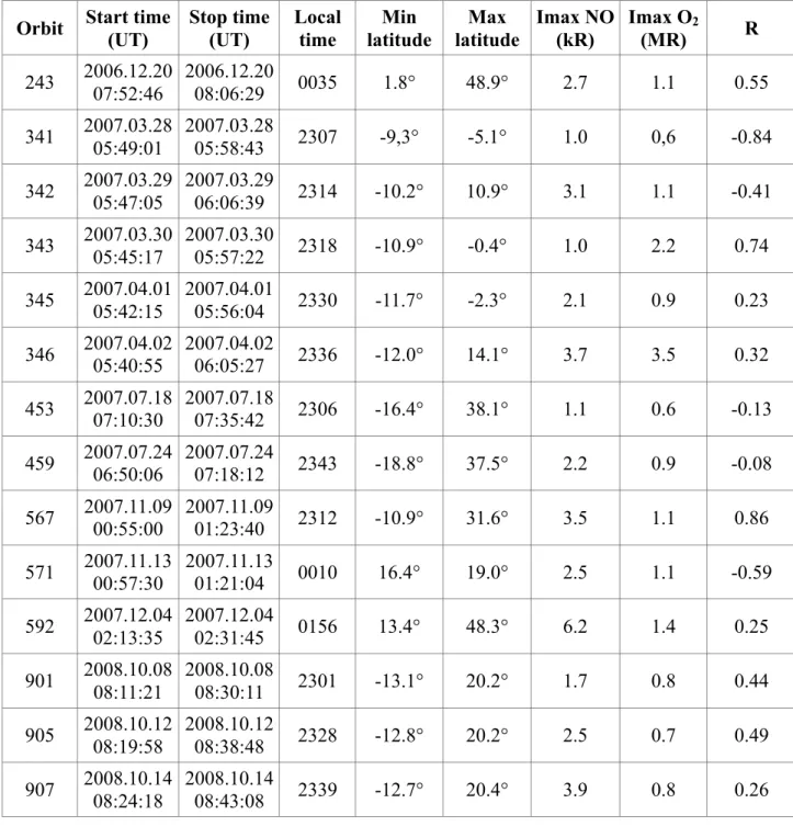
Orbit Start time (UT) Stop time (UT) Local time Min latitude Max latitude Imax NO (kR) Imax O2 (MR) R 243 2006.12.20 07:52:46 2006.12.20 08:06:29 0035 1.8° 48.9° 2.7 1.1 0.55 341 2007.03.28 05:49:01 2007.03.28 05:58:43 2307 -9,3° -5.1° 1.0 0,6 -0.84 342 2007.03.29 05:47:05 2007.03.29 06:06:39 2314 -10.2° 10.9° 3.1 1.1 -0.41 343 2007.03.30 05:45:17 2007.03.30 05:57:22 2318 -10.9° -0.4° 1.0 2.2 0.74 345 2007.04.01 05:42:15 2007.04.01 05:56:04 2330 -11.7° -2.3° 2.1 0.9 0.23 346 2007.04.02 05:40:55 2007.04.02 06:05:27 2336 -12.0° 14.1° 3.7 3.5 0.32 453 2007.07.18 07:10:30 2007.07.18 07:35:42 2306 -16.4° 38.1° 1.1 0.6 -0.13 459 2007.07.24 06:50:06 2007.07.24 07:18:12 2343 -18.8° 37.5° 2.2 0.9 -0.08 567 2007.11.09 00:55:00 2007.11.09 01:23:40 2312 -10.9° 31.6° 3.5 1.1 0.86 571 2007.11.13 00:57:30 2007.11.13 01:21:04 0010 16.4° 19.0° 2.5 1.1 -0.59 592 2007.12.04 02:13:35 2007.12.04 02:31:45 0156 13.4° 48.3° 6.2 1.4 0.25 901 2008.10.08 08:11:21 2008.10.08 08:30:11 2301 -13.1° 20.2° 1.7 0.8 0.44 905 2008.10.12 08:19:58 2008.10.12 08:38:48 2328 -12.8° 20.2° 2.5 0.7 0.49 907 2008.10.14 08:24:18 2008.10.14 08:43:08 2339 -12.7° 20.4° 3.9 0.8 0.26 ! &*'! ! &*(! ! &*)! ! &**!
! ")! Figure captions
'++! '+#!
Figure 1: spatial coverage of SPICAV (in grey) and VIRTIS-M (in black) nadir observations '+"!
of the Venus nitric oxide and O2 (1&) airglow during Venus Express orbit 243.
'+$! '+%!
Figure 2: examples of concurrent observations of the latitudinal distribution of nightglow '+&!
intensities at nadir by VIRTIS-M and SPICAV as a function of latitude: (a) orbit 243, (b) '+'!
orbit 592, (c) orbit 342, (d) orbit 459. Note the different brightness scales used for the NO and '+(!
the O2 airglow emission rates. The brightness at 1.27 µm has been corrected for backscattered
'+)!
emission and both emission rates have been corrected for the view angle. '+*!
! '#+!
Figure 3: sketch illustrating the methodology to generate the data point for the study of the O2
'##!
and NO concurrent limb observations shown in Figures 5 and 6. The projection of the '#"!
SPICAV field of view in the atmosphere is represented by the yellow dotted line. The green '#$!
dotted line shows the parallel line shifted downward by a distance "h along which the values '#%!
of the O2 intensity is extracted to trace emission limb profiles such as illustrated in Figure 4.
'#&! '#'!
Figure 4: example of concurrent limb profiles of the nitric oxide and O2 infrared airglow
'#(!
measured during Venus Express orbit 323. '#)!
'#*!
Figure 5: altitude distribution of the emission peaks of the NO and O2 (1") airglow layers
'"+!
measured quasi-simultaneously at the limb. The observations corresponding to each point '"#!
have been collected as illustrated in Figures 3 and 4 (see text). The dashed line indicates '""!
equal altitudes for the two airglow emission peaks. The correlation coefficient is -0.05, '"$!
! "*! indicating the lack of co-variation of the altitude of the two emissions. The full square '"%!
indicates the mean value of the peak altitude of the two emissions. '"&!
! '"'!
Figure 6: brightness distribution of the emission peaks of the NO and O2 (1") airglow layers
'"(!
measured quasi-simultaneously at the limb. The observations corresponding to each point '")!
have been determined as illustrated in Figures 3 and 4 (see text). The correlation coefficient is '"*!
0.29, indicating the lack of co-variation of the brightness of the two emissions. The full '$+!
square indicates the mean value of the peak intensity of the two emissions. '$#!
'$"!
Figure 7: sketch illustrating the role of horizontal wind in the mesosphere-thermosphere '$$!
transition region as a source of spatial de-correlation between a bright spot of NO airglow and '$%!
a region of enhanced O2 (1") nightglow. The region initially enriched in oxygen atoms has
'$&!
traveled a horizontal distance "L by the time the blob of O-rich gas reaches the altitude of the '$'!
O2 nightglow layer located "z km below the O2 emission peak.!
! "#! Figure 1!! ! ! ! !
! "$! ! ! ! ! ! ! ! %&'()*!+
! "+! Figure 3
! ""! Figure 4
! ",! Figure 5
! "-! Figure 6
! ".! Figure 7