Semi-empirical correlation to model heat losses along solar parabolic trough collectors

PROCEEDINGS OF ECOS 2015 - THE 28TH _{INTERNATIONAL CONFERENCE ON} EFFICIENCY, COST, OPTIMIZATION, SIMULATION AND ENVIRONMENTAL IMPACT OF ENERGY SYSTEMS JUNE 30-JULY 3, 2015, PAU, FRANCE

Semi-empirical correlation to model heat losses

along solar parabolic trough collectors

Rémi Dickesa, Vincent Lemorta and Sylvain Quoilina

a _{Energy Systems Research Unit}

Aerospace and Mechanical Engineering Department Faculty of Applied Sciences

University of Liège Belgium

Contact: rdickes@ulg.ac.be

Abstract:

Solar thermal power plants convert sunshine energy into useful heat and electricity by means of solar collectors and a thermodynamic cycle. Among the different solar collector technologies, parabolic troughs are nowadays the most widespread together with solar towers. In order to improve the computation speed required to simulate the temperature profile along solar parabolic trough collectors, a correlation estimating the effective heat losses of the receiver is an essential tool. However, the relations found in the literature lack accuracy and do not translate effectively the effects of the operating conditions in all cases. In this work, an alternative correlation is proposed and calibrated with the results of a deterministic model. Better fitting performance is demonstrated when compared to the prediction of the pre-existing correlations. The benefits and limitations of the new correlation are finally assessed.

Keywords:

Concentrated solar power, Parabolic trough collectors, Heat losses modeling

1. Introduction

Because of the depletion of fossil fuels and global warming issues, the world of energy is undergoing many changes toward increased sustainability. Among the different technologies being developed, solar energy, including concentrated solar power (CSP) systems, is expected to play a key role to supply electrical demand in medium- and long-terms future [1, 2]. A standard CSP plant uses solar collectors and a tracking system to concentrate direct solar radiation onto a heat collection element (HCE) during sunshine hours. By means of a heat transfer fluid (HTF) flowing in a tube receiver, the concentrated beam is used as heat source for powering a thermodynamic cycle.

2

Among the CSP technologies available, parabolic trough collectors (PTCs), illustrated in Fig. 1, are the most widespread today (with around 95% of the total installed operational concentrating solar power) and is the most promising technology to be developed in the future together with solar towers [3, 4].

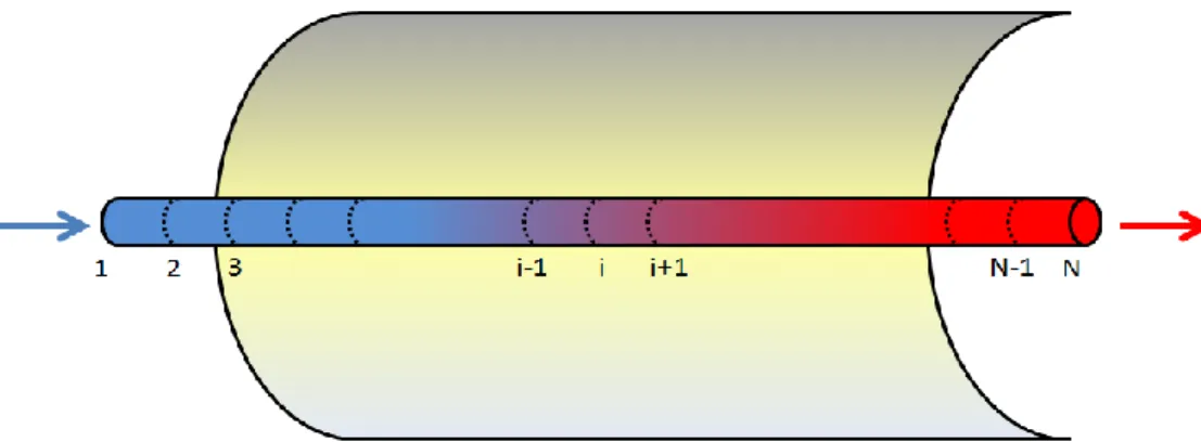
Different methods have been proposed to simulate the HTF temperature at the solar field outlet. Most of them are based on a one-dimensional discretization of the tube receiver along its axial axis, as depicted in Fig. 2. This approach is justified by the large ratio between length and diameter of the heat collection element [5]. Using this methodology, the heat collection element is discretized in N cells of constant volume and the temperature profile along the collectors is evaluated at each node i.e.

𝑇_𝑖+1= 𝑇_𝑖+ 𝑄̇𝑎𝑏𝑠,𝑖

𝑚̇ 𝑐𝑝𝐻𝑇𝐹,𝑖 , ∀𝑖 ∈ [1, 𝑁 − 1] (1)

where 𝑇_𝑖 is the fluid temperature of the ith node, 𝑄̇_{𝑎𝑏𝑠,𝑖} is the net heat power absorbed in the ith cell, 𝑚 ̇is the HTF mass flow rate and 𝑐𝑝_𝐻𝑇𝐹 is the fluid specific heat capacity. In this work, an alternative correlation to easily evaluate the effective heat power transferred to the fluid is proposed. The next section gives a short overview of the current state of the art. Afterward, the alternative correlation is described and its benefits and limitations are discussed.

2. State of the art

The net heat power absorbed by the fluid in each cell, 𝑄̇_{𝑎𝑏𝑠,𝑖} in (1), can be derived by evaluating the radial heat balance of the HCE, as illustrated in Fig.3. This work has been done by Forristal [6] who implemented in EES a deterministic model accounting for each convective, conductive and radiative heat exchanges occurring between the different HCE components and the surrounding environment. Forristal’s deterministic model takes into account the collector optical properties and its geometry, the heat transfer fluid properties and the ambient conditions. It has been validated with experimental datasets [6, 7] and is nowadays widely used in the scientific literature. However, solving such system of equations at each node is computationally-intensive, especially when the number of nodes is high [8].

3

Fig. 2. Radial heat balance of a heat collection element made of an absorber pipe and a glass envelope [6].

An alternative method used to increase the simulation speed is to compute the effective heat losses on each cell, 𝑄̇_{𝑙𝑜𝑠𝑠,𝑖}, by means of a calibrated correlation expressing the linear heat losses HL (in W/m) along the collector in function of different operating variables. Three examples of such correlation - i.e. proposed by Patnode [9], Lippke [10] and Burkholder [7, 11] - are presented hereunder:

𝐻𝐿_{𝑃𝑎𝑡𝑛𝑜𝑑𝑒} = 𝑎₀+ 𝑎₁𝑇_ℎ𝑡𝑓+ 𝑎₂𝑇_ℎ𝑡𝑓2+ 𝑎₃𝑇_ℎ𝑡𝑓3+ 𝑎₄ 𝐷𝑁𝐼 𝑐𝑜𝑠(𝜃) + 𝑎₅ 𝐷𝑁𝐼. 𝑐𝑜𝑠(𝜃) 𝑇_ℎ𝑡𝑓2 (2)

𝐻𝐿_{𝐿𝑖𝑝𝑝𝑘𝑒} = 𝑎₀ + 𝑎₁(𝑇_ℎ𝑡𝑓− 𝑇_𝑎𝑚𝑏) + 𝑎₂ 𝑣_{𝑤𝑖𝑛𝑑}(𝑇_ℎ𝑡𝑓− 𝑇_𝑎𝑚𝑏) + 𝑎₃(𝑇_ℎ𝑡𝑓− 𝑇_𝑎𝑚𝑏)2 ₍₃₎

𝐻𝐿𝐵𝑢𝑟𝑘ℎ𝑜𝑙𝑑𝑒𝑟 = 𝑎0 + 𝑎1 (𝑇ℎ𝑡𝑓− 𝑇𝑎𝑚𝑏) + 𝑎2𝑇ℎ𝑡𝑓2+ 𝑎3𝑇ℎ𝑡𝑓3+ 𝑎4 𝐷𝑁𝐼 𝑐𝑜𝑠(𝜃) 𝑇ℎ𝑡𝑓2+ 𝑎6 √𝑣𝑤𝑖𝑛𝑑+ 𝑎7 √𝑣𝑤𝑖𝑛𝑑 (𝑇ℎ𝑡𝑓− 𝑇𝑎𝑚𝑏) (4)

where 𝑇ℎ𝑡𝑓 (°C) is the fluid temperature, 𝑇𝑎𝑚𝑏 (°C) is the ambient temperature, 𝐷𝑁𝐼 (W/m²) is the direct solar irradiance , 𝜃 is the incidence angle and 𝑣_{𝑤𝑖𝑛𝑑} (m/s) is the surrounding wind speed. The coefficients 𝑎_𝑖 are parameters calibrated to fit experimental data or results given by a deterministic model. Using one of these correlations, the net heat power absorbed by the fluid in each cell, 𝑄̇𝑎𝑏𝑠,𝑖 in (1), can be easily derived by the following set of equations, i.e. 𝑄̇_{𝐿𝑜𝑠𝑠,𝑖} = 𝐻𝐿_𝑖 . ∆𝑥 (5)

𝑄̇𝑆𝑢𝑛,𝑖 = 𝐷𝑁𝐼 . cos(𝜃). 𝜂𝑜𝑝𝑡. 𝑊𝑃𝑇𝐶. ∆𝑥 (6)

𝑄̇𝑎𝑏𝑠,𝑖 = 𝑄̇𝑆𝑢𝑛,𝑖− 𝑄̇𝑙𝑜𝑠𝑠,𝑖 (7)

4

where 𝑄̇_{𝑆𝑢𝑛,𝑖}(W) is the effective solar power reflected, 𝑊_𝑃𝑇𝐶 (m) is the solar collector aperture, 𝜂𝑜𝑝𝑡 is the overall optical efficiency, 𝜌𝑃𝑇𝐶 is the mirror reflectivity, 𝜏𝑒𝑛𝑣𝑒𝑙𝑜𝑝 is the envelop

transmittance, 𝛼𝑡𝑢𝑏𝑒 is the tube absorptivity, and, finally, ∆𝑥 (m) is the discretization step size along

the receiver length.

To evaluate the goodness of the three correlations given in (2), (3) and (4), the coefficients 𝑎_𝑖 are calibrated with the results of a parametric study performed with Forristal’s deterministic model. The resulting coefficients are provided in Appendix. By varying the fluid temperature, the solar irradiance, the wind speed and the ambient temperature, the linear heat losses in 4900 points covering a wide range of operating conditions are evaluated. The parametric inputs chosen for this database are listed hereunder:

 HTF temperature 𝑇_ℎ𝑡𝑓: 30, 42, 55, 67, 79, 92, 104, 116, 129, 141, 153, 165, 178, 190 °C

 DNI: 1, 70, 140, 210, 275, 345, 415, 485, 555, 625, 695, 760, 830, 900 W/m²  𝑣𝑤𝑖𝑛𝑑: 0.5, 2.8, 5.25, 7.6 and 10 m/s

 𝑇𝑎𝑚𝑏: 10, 17.5, 25, 32.5 and 40 °C

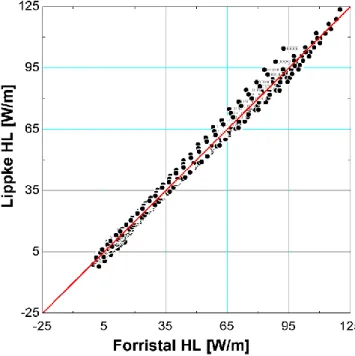
The constant inputs of the parametric study are summarized in Table 1 and are based on the Soponova® parabolic trough collectors produced by Sopogy Inc. [12]. The results predicted by each correlation are compared to the effective heat losses modeled by Forristal’s deterministic model, as shown in Fig. 4. Patnode’s correlation significantly lack of accuracy by only taking the fluid temperature into account. Lippke’s and Burkholder’s correlation show better fitting performance but still do not account for some effects as can be seen in the enlarged view provided in Fig. 4d. A deeper investigation shows that these two correlations do not translate effectively the influence of the solar irradiance and the surrounding wind speed. An alternative form of correlation to evaluate the linear heat losses occurring in parabolic trough collectors is therefore relevant and is presented in the next section.

Table 1. Soponova µCSP collector – Technical specification

Properties Value Units

Glass transmittance 0.91 -

Glass emissivity 0.86 -

Glass absorptivity 0.04 -

Glass conductance 1.04 W/m.K

Tube absorptivity 0.95 -

Heat transfer fluid Ehtylen glycol -

PTC aperture 1.425 m

PTC length 3.657 m

Tube inner diameter 23.26 mm

Tube outer diameter 25.4 mm

Envelope inner diameter 51 mm

Envelope outer diameter 55 mm

5 (a) Patnode’s correlation

R² = 94.63 %, RMS =7.3 W/m

(b) Lippke’s correlation

R² = 99. 4 %, RMS = 2.45 W/m

(d) Zoom on Burkholder’s results between 65 and 95 W/m² (c) Burkholder’s correlation

R² = 99.54 %, RMS =2.15 W/m

Fig. 4. Effective vs. predicted linear heat losses with Patnode’s, Lippke’s and Burkholder’s correlations (comparison over 4900 operating conditions)

6

3. Alternative correlation and discussion

As shown in (2), (3) and (4), heat losses in parabolic trough collectors can be estimated with a function of four variables: the fluid temperature 𝑇ℎ𝑡𝑓, the effective solar irradiance 𝐷𝑁𝐼 𝑐𝑜𝑠(𝜃), the

wind speed 𝑣𝑤𝑖𝑛𝑑 and the ambient temperature 𝑇𝑎𝑚𝑏. In order to derive a new correlation, a third

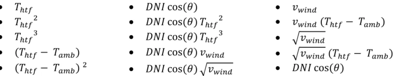
order polynomial equation with cross-terms based on these four variables is used to fit the aforementioned 4900 operating points. Obviously, the resulting expression fits the data very well (R² = 99.98%, RMS= 0.53 W/m) but it requires the calibration of 37 polynomial coefficients. Besides of over-fitting issues, such high number of coefficients results in an impractical expression. To overcome this issue, only the fifteen most relevant terms (i.e. the terms characterized by the highest coefficients in the initial polynomial equation) are selected to be potential candidates in the new correlation. These terms are listed here below:

 𝑇_ℎ𝑡𝑓  𝐷𝑁𝐼 cos(𝜃)  𝑣_{𝑤𝑖𝑛𝑑}

 𝑇_ℎ𝑡𝑓2  𝐷𝑁𝐼 cos(𝜃) 𝑇_ℎ𝑡𝑓2  𝑣𝑤𝑖𝑛𝑑 (𝑇ℎ𝑡𝑓− 𝑇𝑎𝑚𝑏)

 𝑇_ℎ𝑡𝑓3  𝐷𝑁𝐼 cos(𝜃) 𝑇_ℎ𝑡𝑓3  √𝑣𝑤𝑖𝑛𝑑

 (𝑇ℎ𝑡𝑓− 𝑇𝑎𝑚𝑏)  𝐷𝑁𝐼 cos(𝜃) 𝑣𝑤𝑖𝑛𝑑  √𝑣𝑤𝑖𝑛𝑑 (𝑇ℎ𝑡𝑓− 𝑇𝑎𝑚𝑏)

 (𝑇ℎ𝑡𝑓− 𝑇𝑎𝑚𝑏) 2  𝐷𝑁𝐼 cos(𝜃) √𝑣𝑤𝑖𝑛𝑑  𝐷𝑁𝐼 cos(𝜃)

Once these candidates selected, different combinations featuring these terms are investigated to fit the dataset of 4900 operating points. A maximum number of ten terms is imposed in the correlation. Ultimately, the best combination proposed as an alternative correlation to evaluate the linear heat losses in parabolic trough collectors is the following relation:

𝐻𝐿_𝑁𝑒𝑤 = 𝑎₀+ 𝑎₁(𝑇_ℎ𝑡𝑓− 𝑇_𝑎𝑚𝑏) + 𝑎₂ (𝑇_ℎ𝑡𝑓− 𝑇_𝑎𝑚𝑏)2+ 𝐷𝑁𝐼 𝑐𝑜𝑠(𝜃) ( 𝑎₃ 𝑇_ℎ𝑡𝑓2+ 𝑎₄ √𝑣𝑤𝑖𝑛𝑑)

+ 𝑎5 𝑇ℎ𝑡𝑓3+ 𝑣𝑤𝑖𝑛𝑑 (𝑎6+ 𝑎7 (𝑇ℎ𝑡𝑓− 𝑇𝑎𝑚𝑏)) + √𝑣𝑤𝑖𝑛𝑑 (𝑎8+ 𝑎9 (𝑇ℎ𝑡𝑓− 𝑇𝑎𝑚𝑏)) (9)

As it has been done for the three pre-existing correlations given in (2), (3) and (4), the results predicted with the new correlation (9) are compared to the effective linear heat losses simulated by Forristal’s deterministic model, as depicted in Fig. 5. The goodness of fitting is significantly improved with a coefficient of determination (R²) of 99.95 % and a root-mean-square (RMS) lower than 0.8 W/m. The additional terms included in (9) account better for the influence of the solar irradiance and the wind speed on the HCE heat losses, as illustrated in Fig. 5b.

.

7

In the case of a low-temperature solar field (i.e. the HTF temperature remains lower than 200°C), deviations between the different correlations are negligible. As illustrated in Fig. 6, most of the energy losses in these systems are due to optical imperfections (i.e. a mirror reflectivity, an envelope transmittance and a tube absorptivity lower than 1) and the contribution of the heat losses is minor compared to the incident solar energy. The relative error of each correlation compared to the absorbed power in each cell is inconsequential and does not impact significantly the temperature profile along the collectors.

However, in the case of solar fields achieving higher temperature ranges, heat losses become increasingly significant as the HTF temperature increases in tube receiver. Fitting inaccuracies of correlations (2), (3) and (4) can lead to significant errors in the temperature prediction of large-scale solar fields and the additional precision provided by (9) becomes relevant. The new correlation proposed in this contribution can simulate the solar field performance over a wider range of operation, even in strong off-design operating conditions. As an example, Fig. 7 illustrates the temperature profile along the solar field predicted by each correlation during low-radiation solar conditions. The error committed at the solar field outlet is significantly decreased with the new correlation compared to the others. This new correlation is thus a good alternative to better evaluate the temperature profile along parabolic trough collectors.

5. Conclusion

In order to simulate the temperature profile in parabolic trough collectors, the most common approach is based on a 1D discretization of the tube receiver along its axial axis. At each node, the temperature is evaluated by expressing the energy balance on the previous cell of constant volume. In order to calculate the effective heat power absorbed by the fluid, a first method is to solve the radial heat balance in the heat collection element by means of a deterministic model. However, solving this system of equations at each node is computationally-intensive, especially when the number of cells is high. An alternative method is to use a semi-empirical correlation to calculate the effective heat losses occurring along the receiver in order to evaluate the heat power absorbed by

120 130 140 150 160 170 180 190 200 0 200 400 600 800 1000 1200 1400 4 11 18 26 33 40 48 55 62 69 77 84 91 99 106 H TF te m p e ratu re [° C] Li n e ar p o we r [W/m ]

Position along the solar field [m]

Absorbed power [W/m] Optical losses [W/m] Heat losses [W/m] Temperature [°C]

Fig. 6. Temperature profile and power distribution along a low-temperature solar field. (DNI =

8

the fluid in each cell. Three examples of such correlation are found in the literature and compared to a reference deterministic model. A lack of precision is highlighted for all correlations which do not account perfectly for the influence of the operating conditions. An alternative expression is therefore proposed to compute the collector heat losses and the methodology used to derive it is described. The new semi-empirical correlation includes ten terms and it demonstrates better fitting performance to the deterministic model than the pre-existing correlations. Although it is more precise, the additional accuracy provided with the new correlation remains limited for small-scale solar fields in which case most of the energy losses are due to optical imperfections of the collectors. However, in the case of large-scale solar fields, significant heat losses are generated due to the higher temperature range and prediction inaccuracies of the existing correlations can lead to significant simulation errors, especially in strong off-design operating conditions. Therefore, the additional accuracy provided by the new correlation is relevant and it is a good alternative to better evaluate the temperature profile along parabolic trough collectors.

Fig. 7. Temperature profiles evaluated with the different correlations and compared to Forristal’s

result in the case of a low-radiation solar condition (DNI = 5 W/m², NPTC =100).

125 135 145 155 165 175 185 195 0 24 49 73 98 122 146 171 195 219 244 268 293 317 341 366 T empera ture [° C]

Position along the solar field [m]

Forristal Patnode Lippke Burkholder New

𝑇_𝑜𝑢𝑡(°𝐶) ∆𝑇_𝑜𝑢𝑡(°𝐶) Forristal 135.6 - Patnode 142.1 6.5 Lippke 129.2 -6.4 Burkholder 132.2 -3.4 New 136.4 0.8

9

Appendix

The coefficients Ai of the different correlations used to fit the 4900 points described in section 2 are

given in Table 2.

Table 2. Fitting coefficients of the different correlations

Coefficients Lippke’s (3) Patnode’s (2) Burkholder’s (4) New correlation (9)

A0 9.599E+00 -1.268E+01 5.555E+00 2.062E+01

A1 -1.584E-02 4.746E-01 3.856E-01 -2.893E-01

A2 2.826E-03 7.709E-04 4.717E-08 1.472E-03

A3 1.807E-02 3.966E-08 -8.525E-04 2.240E-08

A4 - -3.132E-04 5.777E-06 1.198E-03

A5 - 4.990E-06 -3.937E+00 1.403E-03

A6 - - 9.069E-02 1.045E+00 A7 - - - -3.043E-02 A8 - - - -8.481E+00 A9 - - - 2.073E-01

Nomenclature

CSP Concentrated Solar Power DNI Direct Normal Irradiance HCE Heat Collection Element HTF Heat Transfer Fluid

PTC Parabolic Trough Collectors

Subscripts

abs absorbed amb ambient opt optical tube tube receiver wind surrounding wind

Symbols

𝑐𝑝 Specific heat capacity, J/kg.K 𝐻𝐿 Linear heat losses, W/m 𝑚̇ Mass flow rate, kg/s 𝑄̇ Power, W

𝑇 Temperature, °C 𝑣 Velocity, m/s

10 𝑊 Aperture, m

𝛼 Absorptivity, - 𝜂 Efficiency, - ∆𝑥 Step size, m

𝜃 Incidence angle, rad 𝜏 Transmittance, -

References

[1] Price, H., Hassani, V., Modular Trough Power Plant Cycle and System Analysis. Technical Report NREL/TP-550-31240, 2002, National Renewable Energy Laboratory

[2] International Energy Agency. Article: “How solar energy could be the largest source of electricity by mid-century”, 2014. Available at: < http://www.iea.org>

[3] CSP World, page “WorldMap”.Available at : < http://www.csp-world.com/cspworldmap> [4] Dickes, R., Design and fabrication of a variable wall thickness two-stage scroll expander to

integrated in a micro-solar power plant. 2013. Master Thesis, University of Liège

[5] Dickes, R., Desideri, A., Bell, I., Quoilin, S., Lemort, V., Dynamic modeling and control strategy analysis of a micro-scale CSP plant coupled with a thermocline system for power generation. Conference proceedings. EuroSun 2014, France, September 2014.

[6] Forristal, R., Heat transfer analysis and modeling of a parabolic trough solar receiver implemented in EES. Technical report NREL/TP-550-34169. 2003, National Renewable Energy Laboratory

[7] Burkholder, F., Kutscher C., Heat Loss Testing of Schott’s 2008 PTR70 Parabolic trough receiver. Technical report NREL/TP-550-45633. 2009, National Renewable Energy Laboratory. [8] Dickes, R., Desideri, A., Lemort, V., Quoilin, S., 2015. Model reduction for simulating the dynamic behavior of a micro-solar power system with a thermal storage. Proceedings of the 28th ECOS conference. Under review.

[9] Patnode, A., Simulation and performance evaluation of parabolic trough solar power plants. 2006. Master thesis, University of Wisconsi-Madison.

[10] Lippke, F., The operating strategy and its impact on the performance of a 30 MWe SEGS plant. Journal of Solar Energy Engineering. 1997, Vol. 119, p. 201:207.

[11] Ireland, M., Dynamic modeling and control strategies for a microCSP plant with thermal storage powered by the organic Rankine cycle. 2014. Master thesis, Massachusetts Insitute of Technology.

[12] Sopogy Inc., Soponova µCSP collector datasheet. Available at: <http://www.simonsgreenenergy.com.au/pdf/Data_Sheet_SopoNova_Web.pdf>