The 1958-2008 Greenland ice sheet surface mass balance variability simulated by the regional climate model MAR

(1)

The 1958-2008 Greenland ice sheet surface mass balance

variability simulated by the regional climate model MAR

Xavier Fettweis

(1)(1)

_{, Bruno Franco}

(1)(1)

(1) Laboratoire de climatologie, Université de Liège, Belgium, xavier.fettweis@ulg.ac.be

Abstract.

Abstract. Results made with the regional climate model MAR (Fettweis, 2007) over 1958-2008 show a very high interannual variability of the Greenland ice sheet (GrIS) surface mass balance (SMB) modeled in

average to be 330±125 km³/yr. To a first approximation, the SMB variability is driven by the annual precipitation anomaly minus the meltwater run-off rate variability. Sensitivity experiments carried out by the MAR

model evaluate the impacts on the surface melt of (i) the summer SST around the Greenland, (ii) the snow pack temperature at the beginning of the spring, (iii) the winter snow accumulation, (iv) the solid and liquid summer precipitations and (v) the summer atmospheric circulation. This last one, by forcing the summer air temperature above the ice sheet, explains mainly the surface melt anomalies.

Laboratoire

de climatologie

http://www.climato.be

XY 330

DDSMBSMB ~~ 0,51 D SF_yr - 0,68 D RU (a) ~ ~ 0,62 D SF_yr - 0,60 D PDD_jja (b) ~ ~ 0,74 D SF_yr - 0,48 D TT_jja (c) ~

~ 0,47 D SF_yr-jja + 0,47 D SF_jja - 0,45 D TT_jja (d)

~

~ 0,40 D SF_yr-jja + 0,45 D SF_jja - 0,33 D TT_jun- 0,16 D TT_jul- 0,22 D TT_aug(e) ~

~ 0,55 D SF_yr - 0,36 D Z500_jun- 0,22 D Z500_jul- 0,24 D Z500_aug (f) Corr.= 1.0 RMSE=0.04 Corr.= 0.91 RMSE=0.42 Corr.= 0.92 RMSE=0.39 Corr.= 0.96 RMSE=0.30 Corr.= 0.93 RMSE=0.36 Corr.= 0.97 RMSE=0.26

SMB Surface Mass Balance SF Snowfall RU Run-off

PDD Cumulated Positive Degree Day TT 3m-temperature Z500 yr annual mean June-July-August mean June lean July mean 500hPa geopotential height jja

jun jul

Equation 1.

Equation 1. The time series are centred and normalised. The correlation coefficient (Corr.) and the Root Mean Square Error (RMSE) between the simulated and estimated GrIS SMB anomaly is given. (a)

(a) The Eq 1.a shows that the SMB variability simulated by MAR is mainly driven by the snowfall and the run-off variability. The snow erosion by the wind is not taken into account here but according to Box et al. (2006), its interannual variability is very low.

(b-c)

(b-c) The run-off variability is driven by the cumulated PDD variability which can be estimated by the JJA-mean 3m-temperature according to Fettweis et al. (2008). However, in this estimation, changes in the snow pack properties are not taken into account.

SMB Run-off Snowfall JJA 3m-Temp JJA Z500 Run-off PDD Figure 2.

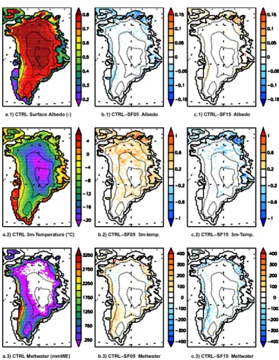
Figure 2. Sensitivity in the MAR model of the a) summer mean 3m-temperature, b) summer mean albedo and c) total meltwater production for a summer snowfall change in the snow model of -50% (SF05) and of +50% (SF15) during the summer 2007 where a record melt was observed (Tedesco et al., 2008). These sensitivity experiments show that higher snowfall during the melt season increases the albedo and consequently decreases the surface melt. The impact of the SF05 (resp. SF15) experiment on the 2007 run-off from the control run (CTRL) is an increase of 9% (resp. a decrease of 7%).

(d)

(d) We tested the inclusion in Eq 1.c of the variability of:

the SST around the GrIS

the snowpack heigh at the end of the spring (low snowpack heigh exposes bare ice and old snow sooner in the season which increases the melt)

the snowpack temperature at the end of the spring (cold snowpack decreases the melt)

the rainfall (high rainfall humidifies the snow and decreases the surface albedo)

but none of them affects the SMB estimation. We only improve the correlation between the simulated and estimated GrIS SMB anomaly time series by splitting the snowfall as in Eq 1.d. Indeed, we estimate then the impact on the melt of the summer snowfall (which temporary increases the surface albedo as shown Fig 2).

(e)

(e) The Eq 1.e shows that it is better to estimate the melt with monthly 3m-temperature variabilities rather than with the JJA-mean 3m-temperature interannual variability which can mask monthly anomalies. Indeed, the melt intensity is not uniformly distributed over the melt season and intensive snow melt can occur only during one of 3 months of the ablation season.

(f)

(f) Finally, the monthly 3m-temperature variability is fully explained by the mi-tropospheric circulation. The 500hPa geopotential heigh gives also information about the precipitation. That is why it is not needed here to split the snowfall as in Eq 1.d.

As conclusion, the SMB variability simulated by the model MAR coupled with a complex energy balance snow model can be reliably approximated by the snowfall variability over the GrIS and by the monthly summer 500hPa geopotential heights induced by the large scale forcing. And then, outputs from global model (e.g. The reanalyses) could be used as proxy of the SMB variability.

References:

- Box, J. E., Bromwich, D. H., Veenhuis, B. A., Bai, L.-S., Stroeve, J. C., Rogers, J. C., Steffen, K., Haran, T., and Wang, S.-H.: Greenland ice sheet surface mass balance variability (1988-2004) from calibrated Polar MM5 output, J. Climate, 19(12), 2783-2800, 2006.

- Fettweis, X.: Reconstruction of the 19792006 Greenland ice sheet surface mass balance using the regional climate model MAR, The Cryosphere, 1, 21-40, 2007.

- Fettweis, X., Hanna, E., Gallée, H., Huybrechts, P., and Erpicum, M.: Estimation of the Greenland ice sheet surface mass balance for the 20th and 21st centuries, The Cryosphere, 2, 117-129, 2008.

-Tedesco, M., Serreze, M., and Fettweis, X.: Diagnosing the extreme surface melt event over southwestern Greenland in 2007, The Cryosphere, 2, 159-166, 2008. SM B a no m al y (k m 3/y r) A no m al y (-) Figure 1.

Figure 1. Top) Time series of the annual total ice sheet SMB, snowfall and run-off simulated by MAR. Units are km³/yr. Bottom) Time series of the GrIS JJA 3m-temperature, cumulated Positive Degree Day (PDD)

simulated by MAR. The mean JJA 500hPa geopotential height simulated by ECMWF (re)analysis is also shown. The time series are centred and normalised (i.e. with standard deviation of 1). Finally, there is the 5-yr running mean in dash. The GrIS gains mass at the surface from the beginning of the 1970's until the middle of the 1990's due to a conjunction of cold and wet years and losses mass in the dry and warm 1960's and in the very warm 2000's summers.

a.1) CTRL Surface Albedo (-) b.1) CTRLSF05 Albedo c.1) CTRLSF15 Albedo

a.2) CTRL 3m-Temperature (°C) b.2) CTRLSF05 3m-temp. c.2) CTRLSF15 3m-Temp.