ANALYTICAL PREDICTION OF THE BEARING RESISTANCE OF BOLTED CONNECTIONS FOR TUBULAR RACKING STRUCTURES

ANALYTICAL PREDICTION OF THE BEARING RESISTANCE OF

BOLTED CONNECTIONS FOR TUBULAR RACKING STRUCTURES

Vittorio Armenanteb, Marina D’Antimoa, Jean-Françoise Demonceaua, Jean-Pierre Jasparta, Massimo Latourb and Gianvittorio Rizzanob

a _{University of Liège, ArGenCo Department, Belgium} b

University of Salerno, Department of Civil Engineering, Italy

Abstract: The aim of this paper is to provide a formulation able to predict the resistance of

simple shear connections realized by fastening a plate to a hollow square section by means of long bolts. The research is motivated by the fact that the rules currently provided by EC3 for defining the bearing resistance of steel connections are limited to the case of stacks of plates, where every plate composing the connection is always restrained out of plane by the adjoining plate or by the bolt head or nut. This is a condition not verified in case of connections realized with long bolts fastening hollow sections. The work is organized in two sections. First, the results of an experimental campaign are presented and successively, the results of a paramet-ric analysis carried out by means of a Finite Element model calibrated on the experimental data are reported. Afterwards, an analytical approach able to include the local buckling effects arising in these kinds of connections is presented, proposing a coefficient for the reduction of the resistance, to be included in the EC3 formulation.

1. Introduction

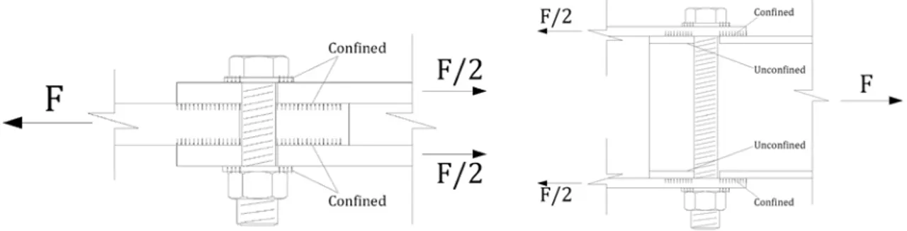
In shelving structures realized by means of hollow section members, a particular system of connection, that has been proposed only recently, consists in bending and drilling the end of the tube composing the beam in order to fasten it to the squared hollow columns with long bolts. Nevertheless, even though such a kind of connection is already used in constructions, it is not among the cases regulated by the Eurocode 3 Part 1.8 [1]. In fact, the rules currently provided by EC3 for defining the bearing resistance of steel connections are limited to the case of stacks of plates, where every plate composing the connection is always constrained out of plane by the adjoining plate or by the bolt head or nut (Fig. 1). This is a condition not verified in case of connections realized with long bolts fastening hollow sections [2]. In fact,

in such connections, the tubes’ faces are constrained out of plane by another plate only in the outward direction, but they are free to buckle inward under the localized action applied by the bolt in shear. These joints have already been subject of a preliminary study of the same au-thors [3], in which it has been pointed out that their behaviour in shear is characterized by a particular failure mode, which is not accounted for in the current formulation provided by EC3. In fact, due to the adoption of tubes with small thickness of the plates and high strength steel, these connections may be characterized by a failure occurring due to the arisement of local buckling phenomena (Fig. 1). Within this framework, the main goal of this paper is to investigate the behaviour of this joint typology, with the aim of providing an analytical for-mula able to predict the shear resistance with an approach in line with the current approach codified by EC3.

Fig. 1: Layout of the tested specimens

Therefore, in order to provide an approach able to extend the formulation proposed by Eu-rocode 3 to connections made with tubular elements and long bolts, a model for determining the value of the critical load leading to the local buckling of the plate composing the steel tube is presented. Such a load is evaluated by studying the behaviour of a sub-structure, idealized by extracting from the whole connection only the end portion of the tube’s plate subjected to a compression load, which is used to simulate the localized bolt action. Furthermore, in order to introduce in the model the constraining action provided by the remaining part of the tube on the considered sub-structure, particular boundary conditions are applied. Such a sub-model is used to evaluate the critical elastic buckling load by performing buckling analyses in SAP 2000. Afterwards, the value of the critical elastic load obtained from the FE analysis is cor-rected by adopting Winter’s approach [4] in order to account for the fact that the local buck-ling occurs in plastic field and to account for the effects related to the geometric imperfec-tions. Exploiting the results of the parametric analysis, a new coefficient to be included in the current EC3 formulation to account for local buckling phenomena arising in case of tubular members fastened with long bolts is proposed. The new coefficient is expressed as a function of the ratio between tube’s thickness and hole diameter.

2. Evaluation of the buckling load

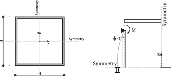
The procedure applied in this work to assess the value of the critical load leading to the local buckling of the tube is carried out starting from the analysis of a sub-structure extracted from the whole connection representative of the zone of the tube where the local buckling effects are more significant. In particular, the sub-structure is idealized by extracting from the tube’s plate only the end portion, whose dimensions are the width of the tube (H) and the distance between the center of the hole and the free edge of the tube (e1) (Fig. 2). This is the zone that, as also demonstrated by the experimental analysis, is more significantly influenced by the lo-cal buckling phenomena.

Fig. 2: Boundary conditions applied

Dealing with the modelling of buckling phenomena, it is well known that the definition of the restraining conditions applied at the edges of the plate is of paramount importance, due to the influence that the constraints have on the value of the critical buckling load. This is the reason why, even though in the present work only a small portion of the tube is studied, the continuity of the analysed plate with the remaining parts of the tube is recovered by consider-ing appropriate boundary conditions applied on the edges of the element (Fig. 2).

In particular, in the following, the considerations made to define the stiffness of appropri-ate springs able to account for the rotational, shear and axial behaviour of the remaining parts of the tube’s plates are described. In particular, in order to account for the remaining portions of the tube the following constraints are applied at the edges of the analysed plate (Fig. 3):

• at the intersection of the edges of the plate with the lateral walls of the tube rotational springs and vertical supports are applied (edges A-B and D-C);

• on the edge loaded under compression by the bolt, in-plane and out-of-plane springs are introduced both on the portions of the edge next to the hole (edges A-F and D-E) and in the corners of the plate (points A and D). Furthermore, in the zone of the hole, a uniform load modelling the shear action transferred by the bolt is introduced;

• at the free edge of the tube no boundary conditions are introduced (edge B-C).

Fig. 3: Scheme used to define the rotational stiffness due to the lateral plates of the tube

F/2 d 0 A B C D E F x y

Vertical supports + Rotational springs

Fre

e e

dg

e

Vertical supports + Rotational springs Spring in Direction x + Support in Direction z Springs in Direction x/z Springs in Direction x/z Spring in Direction x + Support in Direction z H e1 y z Symmetry Sy mmetr y H H y z Symmetry Sy mmetr y M φ=1

Therefore, on the sides of the plate parallel to the load (from A to B and from D to C, Fig. 3), out-of-plane supports and rotational springs are applied in order to model the axial and rota-tional stiffness of the lateral plates of the tube. In particular, in order to model the axial stiff-ness of the lateral plates of the tube, on these edges, the out-of-plane supports are defined as rigid elements. Conversely, the stiffness of the rotational springs is determined by defining the value of the bending moment needed to generate a unitary rotation on the lateral plates of the tube (Fig. 3). By adopting this approach, the following expression is obtained:

, 2 lateral EI k H φ = (1)

where E is the modulus of elasticity of steel, I is the moment of inertia of the lateral tube’s plate per unit of length and H is the height of the tube’s plate.

The side that goes from B to C is considered free; a similar assumption is made for the por-tion of the edge on which the load is applied that goes from E to F. In addipor-tion, in order to ac-count for the stiffness of the remaining part of the tube behind the analysed plate, various con-siderations are made. In particular, at points A and D of the model (the corners of the plate) extensional springs in the x direction accounting for the stiffness of the portion of the lateral plate behind the bolt are applied. The stiffness of such springs is easily calculated as:

, ( lp / 2) x corners E A k L = (2)

where L is the length of the tube and Alp is the area of the lateral wall of tube calculated as the

product of the tube thickness t and H/2. In the same way, in the zone going from A to F and from E to D extensional springs are spread along the edges both in the x and in the y direc-tion. As already made for the stiffness k_{x corners,} , the value of the stiffness of the springs spread on the loaded edge is determined in order to account for the axial deformability of the remain-ing part of the top plate located behind the bolt:

, ( tp/ 2) x edge E A k L = (3)

where Atp is the area of the top plate of the tube calculated as the product of the tube thickness

t and H. Conversely, the stiffness of the springs in the y direction is determined in order to

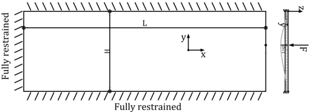
account for the out-of-plane deformability of the portion of the tube behind the bolt hole. To this scope, the simple scheme of plate fully restrained on three edges loaded with a unitary force applied on the free edge represented in Fig.4 has been studied. Therefore, in order to determine the value of the stiffness of the springs to be applied on the holed side of the plate several schemes with the force applied in different points of the free edge have been solved.

Fig. 4: Scheme used to evaluate the out-of-plane stiffness

x y y z Fully restrained Fully restrained Fu lly re str ai ne d F δ =1 H L

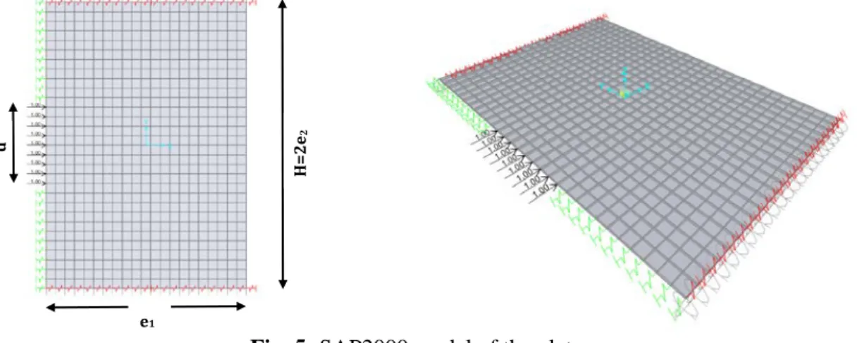
In order to maintain a simple structure of the model and to avoid to introduce a variable value of the springs’ stiffness, the out-of-plane stiffness of the springs has been assumed constant and equal to the value of the force needed to obtain a unitary displacement at the mid-point of the plate’s edge. Conversely, at the corners of the plate, as already said, a fixed support has been applied. This choice is justified by the fact that, from some preliminary analyses, no ap-preciable differences were found in the results considering a variable value of the springs’ stiffness or a constant value. Under the reported hypotheses, the value of the elastic buckling load of the plate with the above described boundary conditions has been determined by devel-oping an appropriate FE model in SAP2000 v.16 software package (Fig.5).

Fig. 5: SAP2000 model of the plate

An example of the results of one of the analyses presented in the next section is delivered in Fig.6, where the shapes of the first two buckling modes of one on the analysed cases are represented. As it is possible to verify, the 1st buckling shape, i.e. the buckling shape charac-terized by the lowest value of the load multiplier, is the one typically observed also in the ex-perimental analysis.

e1=48 mm, H=60 mm, t = 0.50 mm, d=16 mm

1st mode – αcr =105.3 2nd mode – αcr =306.8 Fig. 6: Buckling modes for a plate with thickness equal to 0.50 mm

In order to obtain a value of the critical buckling load representative of the actual conditions of the plate it is necessary to account for two additional parameters that normally provide a significant influence on such a value: the imperfections and the non-linear behaviour of steel. In fact, both these factors, as widely recognized in technical literature, may provide a signifi-cant reduction to the value of the buckling resistance calculated by means of an elastic analy-sis and, therefore, they need to be accounted for in order to obtain a formulation able to pre-dict the ultimate buckling load of the analysed connection. In this work, in order to account for these factors, the empirical approach of Winter [4], already proposed by EC3 [1] and by

e1

d

H=2e

the AISI specifications [5], is followed in order to account for the influence of imperfections and of the non-linear behaviour of the material. Such an approach is based on the application of the effective width concept and provides to correct the value of the plastic load that the plate can carry by means of the following expression:

0, 22 1 1-cr pl pl pl p p N N β N N λ λ    = = _ _ ≤ _{ }    (4) where λ_p is a non-dimensional slenderness parameter expressed as:

1/ 2 pl p cr N F λ _{= } _   (5)

where Fcr is the value of the elastic buckling load, evaluated in this work by means of the

buckling analyses described previously, and Npl is the value of the plastic load. It is worth

noting that, according to the Winter’s methodology, the two coefficients 1 p λ and 0, 22 1-p λ        

reported in Eq. 4 account for the influence of the mechanical non-linearity of the material and for the imperfections respectively [4,6] The value of the plastic load Npl is determined

accord-ing to the formulation currently proposed by EC3 part 1.8 under the hypothesis of full plasti-cization of the plate:

, 2.5

b Rd u

F = f td (6)

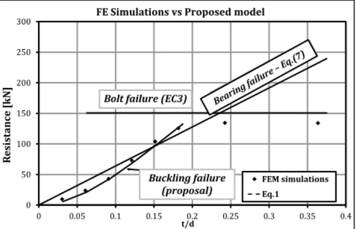
The accuracy of the model herein describer has been checked against some of the experi-mental and FE results currently available and described in another work of the same authors (D’Antimo et al., 2016). In Fig. 7 the values of the maximum loads calculated in the experi-mental and numerical activity developed in D’Antimo et al. (2016) are compared with those calculated by means of the proposed model and with those calculated by means of the EC3 approach. In particular, in the picture, with a black dot are reported the values of the maxi-mum load calculated in D’Antimo et al. (2016), with a continuous line are represented the values of the bearing resistance of the plate calculated according to the EC3 model, with a dashed and dotted line are represented the values of the bolt resistance calculated according to EC3 model and with a simple dashed line are represented the values of the buckling load cal-culated with the model proposed in this paper. From such a figure it is easy to observe that in the buckling range the proposed model is able to predict the load values more accurately than EC3. Conversely, for higher values of the t/d ratio other failure modes become more signifi-cant and, therefore, EC3 provides a higher accuracy in the prediction.

Fig. 7: Mathematical model vs. FE simulation

0 50 100 150 200 250 300 0 0.05 0.1 0.15 0.2 0.25 0.3 0.35 0.4 Re si st an ce [kN ] t/d FEM simulations Eq.1

Bolt failure (EC3)

Buckling failure (proposal)

In addition, it is also possible to observe that the resistance of the connection is accurately predicted in the whole range of analysed values if the resistance is calculated as minimum of the resistance of the three possible failure mechanisms. Therefore, starting from this observa-tion, in the next section a proposal of improvement of the EC3 approach including the local buckling failure mode of the plate by means of the approach proposed in this paper, is de-scribed.

3. Proposal of an improvement to EC3 approach

According to Eurocode 3, the bearing resistance of a shear connection is provided by the fol-lowing relationships: , b Rd b u F = kα f td (7) 1 0 ; ;1 3 ub b u f e min d f α = _ _   (8)

where, fu and fub are respectively the plate and bolt ultimate strength, d is the bolt diameter, e1

is the distance of the hole from the plate free edge and k is a parameter accounting for the in-fluence of the lateral distance on the tear-out failure mode. Typically, such a factor, for a flat plate, depends on the distance between the hole and the lateral edge e2 and is equal to 2.5

provided that e2 is greater than 1,5d0. In case of tubes, as already demonstrated in D’Antimo

et al. (2016), in order to apply the EC3 formulation, the k factor has to be directly assumed equal to 2.5. In fact, in case of tubular sections, the presence of the side walls allows to ne-glect the influence of the reduction of resistance arising for small values of the distance of the hole from the free edge (e2<1.5d0). Eqs. 7-8, account for all the basic failure modes normally arising in a simple bolted connection and, in particular, include the tear-out, bearing and shear failure mechanisms. Basing on the procedure for determining the critical buckling load of plates of tubular members reported in previous sections, the aim of this section is to provide an additional coefficient to be included in Eqs.7-8 to account for the possibility of local buck-ling failures mode (Fig.1). In particular, with the aim to keep the same structure of the code equation, the idea is to propose to include in coefficient 𝛼_𝑏 of Eq. 8 an additional factor to be properly calibrated by means of a parametric analysis. To this scope, equating the ratio be-tween the ultimate bearing resistance provided by Eq. 5 and that calculated by means of Eq. 1 to one a new factor 𝛼_{𝑏,𝑠𝑡} to be added in the classical bearing resistance formula can be de-fined: , , , 2.5 1 2.5 b Rd b st u cr Rd u F dtf N dtf α β = = (9) , b st α =β (10) where 1 0, 22 1 p p β λ λ   = −_ _

  is the buckling factor evaluated according to Winter’s formula. Therefore, following this approach, in order to find a simple formula to be used in design, the main issue is to define a correlation between β and the main geometrical parameters of the analysed connection. According to what is reported before, the factors that may influence sig-nificantly the load in case of buckling failure mode are t/d, e1/d and e2/d ratios. Therefore, the

parametric study proposed in this section has been mainly devoted to investigate the influence of these three parameters on the value of β.

Table 3: Results of the parametric analysis

1st group of analyses – influence of t/d t/d e1/d e2/d d [mm] t [mm] e1 [mm] e2 [mm] Ncrit,FEM [kN] fy/fu [MPa] Npl [kN] λp [Eq.2] β Ncr,rd [kN] 0.05 3 2.5 16 0.8 48 40 3.51 443/499 15.97 2.134 0.420 6.711 0.075 3 2.5 16 1.2 48 40 11.84 443/499 23.95 1.422 0.594 14.235 0.1 3 2.5 16 1.6 48 40 28.08 443/499 31.94 1.067 0.744 23.767 0.125 3 2.5 16 2 48 40 54.84 443/499 39.92 0.853 0.870 34.724 0.15 3 2.5 16 2.4 48 40 94.77 443/499 47.90 0.711 0.971 46.529 0.05 3 2.5 12 0.6 36 30 1.86 443/499 8.98 2.195 0.410 3.682 0.075 3 2.5 12 0.9 36 30 6.30 443/499 13.47 1.462 0.581 7.829 0.1 3 2.5 12 1.2 36 30 14.95 443/499 17.96 1.096 0.729 13.099 0.125 3 2.5 12 1.5 36 30 29.20 443/499 22.46 0.877 0.854 19.182 0.15 3 2.5 12 1.8 36 30 50.46 443/499 26.95 0.731 0.956 25.773

2nd group of analyses – influence of e1/d

0.1 3 2.5 16 1.6 48 40 26.976 443/499 31.94 1.088 0.733 23.417 0.1 3.5 2.5 16 1.6 56 40 27.365 443/499 31.94 1.080 0.737 23.542 0.1 4 2.5 16 1.6 64 40 27.558 443/499 31.94 1.077 0.739 23.604 0.1 4.5 2.5 16 1.6 72 40 27.684 443/499 31.94 1.074 0.740 23.644 0.2 3 2.5 16 3.2 48 40 212.934 443/499 63.87 0.673 1.000 63.882 0.2 3.5 2.5 16 3.2 56 40 218.957 443/499 63.87 0.673 1.000 63.882 0.2 4 2.5 16 3.2 64 40 220.512 443/499 63.87 0.673 1.000 63.882 0.2 4.5 2.5 16 3.2 72 40 221.516 443/499 63.87 0.673 1.000 63.882 0.3 3 2.5 16 4.8 48 40 718.672 443/499 95.81 0.673 1.000 95.823 0.3 3.5 2.5 16 4.8 56 40 739.028 443/499 95.81 0.673 1.000 95.823 0.3 4 2.5 16 4.8 64 40 744.221 443/499 95.81 0.673 1.000 95.823 0.3 4.5 2.5 16 4.8 72 40 747.638 443/499 95.81 0.673 1.000 95.823

3rd group of analyses – influence of e2/d

0.031 3 1.9 16 0.5 48 30 0.948 443/499 9.98 3.245 0.287 2.867 0.063 3 1.9 16 1 48 30 7.59 443/499 19.96 1.622 0.533 10.638 0.094 3 1.9 16 1.5 48 30 25.59 443/499 29.94 1.082 0.736 22.051 0.125 3 1.9 16 2 48 30 60.69 443/499 39.92 0.811 0.899 35.870 0.16 3 1.9 16 2.5 48 30 118.53 443/499 49.90 0.673 1.000 49.908 0.0313 3 2.5 16 0.5 48 40 0.698 443/499 10.00 3.784 0.249 2.488 0.05 3 2.5 16 0.8 48 40 3.51 443/499 15.97 2.134 0.420 6.711 0.075 3 2.5 16 1.2 48 40 11.84 443/499 23.95 1.422 0.594 14.235 0.1 3 2.5 16 1.6 48 40 28.08 443/499 31.94 1.067 0.744 23.767 0.125 3 2.5 16 2 48 40 54.84 443/499 39.92 0.853 0.870 34.724 0.15 3 2.5 16 2.4 48 40 94.77 443/499 47.90 0.711 0.971 46.529 0.0313 3 3.5 16 0.5 48 56 0.51 443/499 10.00 4.420 0.215 2.149 0.05 3 3.5 16 0.8 48 56 2.402 443/499 15.97 2.578 0.355 5.665 0.075 3 3.5 16 1.2 48 56 7.115 443/499 23.95 1.835 0.480 11.489 0.1 3 3.5 16 1.6 48 56 16.774 443/499 31.94 1.380 0.609 19.455 0.125 3 3.5 16 2 48 56 32.77 443/499 39.92 1.104 0.725 28.961 0.15 3 3.5 16 2.4 48 56 56.62 443/499 47.90 0.920 0.827 39.624 0.05 3 4.5 16 0.8 48 72 1.651 443/499 15.97 3.110 0.299 4.771 0.075 3 4.5 16 1.2 48 72 5.908 443/499 23.95 2.013 0.442 10.596 0.1 3 4.5 16 1.6 48 72 13.209 443/499 31.94 1.555 0.552 17.633 0.125 3 4.5 16 2 48 72 25.820 443/499 39.92 1.243 0.662 26.425 0.15 3 4.5 16 2.4 48 72 44.617 443/499 47.90 1.036 0.760 36.416 0.2 3 4.5 16 3.2 48 72 105.766 443/499 63.87 0.777 0.923 58.923 0.225 3 4.5 16 3.6 48 72 150.584 443/499 71.86 0.691 0.987 70.892 0.25 3 4.5 16 4 50 72 206.493 443/499 79.84 0.673 1.000 79.853

The analyses have been performed by carrying out three groups of simulations. A first group, devoted to investigate the influence of the t/d ratio. In this case the analyses have been carried out by fixing the values of e1/d equal to 3 and of e2/d equal to 2.5 and by varying the bolt

di-ameter d and plate thickness t singularly. In particular, in this first group of analyses the val-ues of d have been assumed equal to 12 and 16 mm and the t/d ratio has been varied in the range 0.05/0.15. The second group of analyses has been carried out in order to investigate the influence of the e1/d ratio. In this case the analyses have been carried out by fixing the value

of e2/d equal to 2.5 and by varying t/d in between 0.1 and 0.3 and e1/d in between 3 and 5.

The third group of analyses has been carried out with the aim to investigate the dependence of the buckling resistance on the parameter e2/d. In this case e2/d has been varied in between

1.88 and 3.5, t/d has been varied in the range 0.03 and 0.15 and e1/d has been fixed as equal

to 3. For each of the analysed cases, the procedure previously reported to determine the value of the inelastic buckling load has been applied and, subsequently, the value of the critical elas-tic buckling load and the value of the reduction factor calculated by means of the Winter’s approach have been calculated. The results of these analyses are summarized in Table 3.

4. Conclusions

In this work the behaviour of connections made with SHS and long bolts has been investigat-ed. The analysis performed in this paper has been devoted to develop a design formula able to account for the particular buckling failure mode arising in these connections. First of all, in order to define this formula, a procedure able to predict the critical load of the tube’s plate under the action applied by the bolt has been set up. This procedure has been based on the study of the portion of the plate, which is mainly influenced by the buckling phenomena by defining, in order to recover the restraining action due to the remaining parts of the tube, ap-propriate boundary conditions. The buckling load of the studied plate has been evaluated by first performing a buckling analysis in SAP2000 and by after correcting the value of the criti-cal load by means of the Winter’s approach in order to account for imperfections and for the plastic behaviour of steel. This procedure has been validated against the available data re-trieved from the tests and analysis performed in [3]. Afterwards a parametric analysis has been carried out in order to find a correlation between the reduction of resistance due to the buckling failure mode and the geometrical properties of the tube’s plate. The analysis has shown that the local buckling effects, in the analysed connection, may be significant depend-ing on the values of t/d and of e2/d demonstrating that the buckling check is required if t/d is

lower than 0.018e2/d+0.124. Using the results of the parametric analysis a coefficient able to

account for the bucking failure mode to be included in EC3 has been defined.

References

[1] CEN (2005). Eurocode 3: Design of steel structures - Part 1-8: Design of joints. European Committee for Standardization, CEN, Brussels.

[2] Hoang VL, Jaspart JP, Demonceau JF. “Extended end-plate to concrete- filled rectangular column joint using long bolts”, Journal of Constructional Steel Research, 113, 2015.

[3] D’Antimo M. “Experimental and theoretical analysis of shear bolted connections for tubular racking structures”, under Review on Engineering Structures.

[4] Winter G. “Strength of thin steel compression flanges”, Reprint No. 32, Ithaca, NY, USA: Cornell University Engineering Experimental Station.

[5] AISI (1996). Specification for the design of cold formed steel structural members. New York: American Iron and Steel Institute.

[6] Von Karman T. “Festigheitsprobleme im Maschinenbau”. Encyclopaedie der