A Review of Fluid Forces Induced by a Circular Cylinder Oscillating at Low Amplitude and High Frequency in Cylindrical Confinement

HAL Id: hal-01380380

https://hal.archives-ouvertes.fr/hal-01380380

Submitted on 13 Oct 2016

HAL is a multi-disciplinary open access

archive for the deposit and dissemination of

sci-entific research documents, whether they are

pub-lished or not. The documents may come from

teaching and research institutions in France or

abroad, or from public or private research centers.

L’archive ouverte pluridisciplinaire HAL, est

destinée au dépôt et à la diffusion de documents

scientifiques de niveau recherche, publiés ou non,

émanant des établissements d’enseignement et de

recherche français ou étrangers, des laboratoires

publics ou privés.

Distributed under a Creative Commons Attribution| 4.0 International License

A Review of Fluid Forces Induced by a Circular

Cylinder Oscillating at Low Amplitude and High

Frequency in Cylindrical Confinement

Cedric Leblond, Jean-François Sigrist, Christian Laine, Bruno Auvity, Hassan

Peerhossaini

To cite this version:

Cedric Leblond, Jean-François Sigrist, Christian Laine, Bruno Auvity, Hassan Peerhossaini. A Review

of Fluid Forces Induced by a Circular Cylinder Oscillating at Low Amplitude and High Frequency in

Cylindrical Confinement. ASME 2006 Pressure Vessels and Piping/ICPVT-11 Conference, Jul 2006,

Vancouver, Canada. pp.45-54, �10.1115/PVP2006-ICPVT-11-93017�. �hal-01380380�

A REVIEW OF FLUID FORCES INDUCED BY A CIRCULAR CYLINDER

OSCILLATING AT LOW AMPLITUDE AND HIGH FREQUENCY IN CYLINDRICAL

CONFINEMENT.

Cedric Leblond

Service Technique et Scientifique DCN Propulsion

Indret - BP 30

44620 LA MONTAGNE, FRANCE Email: cedric.leblond@dcn.fr

Jean Francois Sigrist Christian Laine

Service Technique et Scientifique DCN Propulsion Indret - BP 30 44620 LA MONTAGNE, FRANCE Bruno Auvity Hassan Peerhossaini Laboratoire de Thermocinetique CNRS UMR 6607 Rue C. Pauc - BP 50609 44306 NANTES, FRANCE ABSTRACT

This paper deals with fluid forces induced by an oscillating rigid circular cylinder in a fluid initially at rest. The amplitude of the imposed movement is assumed sufficiently small so that no wake is formed. The objective of the present paper is to re-view different theoretical methods to evaluate fluid forces. A wide variety of conditions is considered, from inviscid, compressible flows in infinite fluid domains, to viscous, incompressible and strongly confined ones. A special care is taken to underline the limits of the simplified models regarding real fluid effects, such as three-dimensional centrifugal instabilities. This review is re-lated to a study whose ultimate aim is to predict dynamic fluid load during a typical shock encountered in the environment of a military ship.

INTRODUCTION

The patterns induced by a bluff body undergoing harmonic oscillation in a direction normal to its axis in a still fluid are of considerable fundamental and engineering interest. If the ampli-tude of the body is high enough, the boundary layer can break away from the body surface by a phenomenon called separa-tion [1, 2]. Vortices are then generated in each half cycle, re-sulting in different wakes formation [3, 4]. These vortices can strongly influence the fluid force experienced by the body [5–7]. This paper focuses on the regimes induced by sufficiently small displacements of the body so that no separation occurs in the

fluid flow [5]. The study of these regimes have several practi-cal applications. In infinite fluid domains, they can yield to the prediction of the loading on ocean structures exposed to waves. In confined fluid domains, they are specially of interest in fields such as heat exchanger and squeeze film dampers design [8–11]. In case of shock loading, naval components are subjected to high acceleration and frequency motions. These components can be in contact with a viscous fluid. In order to improve design margins and ensure security, long life and satisfactory operating performance of the components, the precise knowledge of the fluid effects on solids is of major importance [12]. In particular, the sources of damping have to be well characterized since they can limit the vibrations of the structures.

A R×D program has been launched by DCN Propulsion in order to obtain some insights into real flow effects. It consists of studying the flow induced by a circular cylinder moving in a direction normal to its axis in a fluid initially at rest. A first approach was to consider added mass effects in fully coupled fluid-structure problems [13, 14]. Interest was put on harmonic oscillations in a cylindrically confined fluid. A second approach was to take into account some history effects in an infinite fluid medium surrounding a rigid circular cylinder [15]. The motion of interest was then a displacement induced by an unique sinu-soidal period of acceleration imposed to the cylinder. The next steps are to consider complex phenomena such as unsteady sep-aration, inertial effects in lubricant films and three-dimensional

Figure 1. THE GEOMETRICAL CONFIGURATION.

instabilities.

The development of new measuring techniques (Particle Im-age Velocimetry for example) and the increased hardware perfor-mance can now provide detailed information about the time vari-ation of local flow properties. Literal expressions of fluid forces [16–18] can then be used to make the link between these prop-erties and the time-dependent loading of structures. The most convenient expressions are reviewed in the second section. In the section called ”Simplified models” some engineer’s models of fluid force prediction on moving circular cylinder are exposed. Simple effects such as resonance, added mass and damping are highlighted in the case of attached, laminar and two-dimensional flows. The limits of these simple models and some remaining challenges concerning real flow effects are exposed in the last section. They may be numerically out of reach and difficult to appreciate experimentally. Modeling them has already been a major issue for more than fifty years and still represents a huge challenge for the future. In the following of this introduction, the key parameters of the system considered in this paper are pre-sented.

We consider a viscous fluid of densityρconfined in an an-nular region, see Fig. 1. The dynamic viscosity is noted µ =ρν withνthe kinematic viscosity. The speed of sound in the fluid at rest is noted c. The inner circular cylinder of radius R1(and

diameter d = 2R1) is subjected to a harmonic motion e(t) in the

direction exdefined by:

e(t) = emcosωt (1)

The maximum velocity Vm= emωis also used in this paper. The

outer cylinder of radius R2 is at rest. For the case of an

infi-nite fluid medium, it comes R2=∞. When the fluid is

con-sidered as viscous, no-slip boundary conditions are used on the

cylinders, however when the fluid is assumed inviscid, only the normal component of the velocity is conserved on the walls and the fluid is allowed to slip. The length of the cylinders are sup-posed infinite so that end effects may be neglected. Moreover heat transfers and axial flows are not considered in this paper. This study is also restricted to a sufficiently small displacements of the inner circular cylinder so that no wake is formed. There are at least seven independent parameters (R1, R2, em,ω,ν,ρ, c)

for three units (kg, m, s), so the problem is driven by at least four dimensionless numbers. An overview of all possible fluid states in the whole dimensionless numbers space is out of reach so far. Only some particular behaviors will be given. For instance, only subsonic displacement of the inner cylinder is considered:

M =Vm

c << 1 (2)

where M is the Mach number. The interesting dimensionless pa-rameters in this problem depend on the assumptions adopted in each model. For an infinite viscous fluid domain, the flow has historically [5, 19] been characterised by the following dimen-sionless numbers:

β= 1

2π

d2ω

ν the Stokes number (3)

KC = 2πem

d the Keulegan-Carpenter number (4)

In the case of a confined fluid, the Keulegan-Carpenter number is not sufficient to quantify the inner cylinder displacement. So it is convenient to introduce the instantaneous eccentricity ratio

ε(t) defined by the fraction of the eccentricity e(t) with the radial

clearance C = R2− R1. The following dimensionless parameter

can then be formed [20]:

εm= em R1(α− 1) withα=R2 R1 . (5)

For a compressible inviscid flow, βcan not be used in order to quantify the frequency of the imposed movement, and the non-dimensional frequencyΩis preferred:

Ω=R1ω

c . (6)

Surface state effects may also influence the flow behaviour. They are usually characterized using the non-dimensional number k/d where k is the roughness height. However, this ratio is generally not sufficient and the shape of the asperities have to be consid-ered [21–23].

FORCE EXPRESSIONS

Literal fluid forces expressions on a moving body

There are several ways to evaluate fluid forces experienced by a moving body. An extrinsic measurement yields the forces by the precise knowledge of the body trajectory, as in the case of particle-wall collision [24]. It can be achieved by the use of strain and/or displacement gauges. An intrinsic measurement is inferred from the knowledge of the fluid velocity fields and their

derivatives [16]. This latter method has considerable advantages. For instance, it does not required any gauges and allows to mea-sure small force level. Different formulae can be used so as to proceed to an intrinsic method. Some of them are given in what follows. By definition the force acting on the body surface Sb(t)

can be expressed by:

F(t) = Fp+ Fµ= −

Z

Sb(t)

(−p n + ¯¯T · n)ds (7) where Fpand Fµ represent respectively the contribution of the

pressure and the viscous forces, n is the unit normal vector (see Fig. 1) and ¯¯T denotes the viscous stress tensor given by

¯¯

T = µ (∇u + (∇u)T)) with u the local fluid velocity. Even if

Eqn. (7) combines two clearly distinct effects, pressure and vis-cosity, they are not fully decoupled since the fact that the viscos-ity is taken into account can strongly modify the pressure field. As a consequence, the pressure force is generally different from the one obtained with an inviscid flow. Since the viscous force is expressed by velocity derivatives at the boundary, the accuracy of its calculation depends on the resolution at the vicinity of the wall. However, in most experiments, and specially in the case of a moving wall, the flow is not well described at this place. To overcome this issue, Eqn. (7) can be expressed more generally in term of time-dependent control volume V (t) bounded externally by the body surface:

F(t) = −d dt Z V (t)ρ u dV (8) + Z S(t) n · ³ −p ¯¯I−ρ(u − ˙e(t)ex) u + ¯¯T ´ ds

The first term of the right hand side is the time rate change of momentum within the control volume and the second one gath-ers respectively the instantaneous pressure force, the net flux of momentum and the instantaneous shear force on the control sur-face. Sometimes, the knowledge of the pressure distribution is missing, so Eqns. (7,8) are particularly inconvenient. This is the case in computations when the hydrodynamic problem is not cast in velocity-pressure form, but in velocity-vorticity or in streamfunction-vorticity formulation. This is also the case in the experiments when the velocity field is obtained by Particle Image Velocimetry (PIV). Then, either pressure is obtained as a solution of a separate problem or it is removed from Eqn. (8). This latter method can be achieved [17, 25] but may result in the apparition of a geometrical variable. However, both this new variable and the pressure are not directly visible. So as to provide a straight-forward link between the flow patterns and the fluid forces, it can be convenient to reformulate Eqn. (8) with the vorticity fieldωω only. In an infinite fluid domain, it yields [18]:

F(t) = − 1 N − 1ρ d dt Z V (t) x ×ωdV (9) + 1 N − 1ρ d dt Z Sb(t)x × (n × ˙e(t)ex) ds

where N is the spatial dimension and x the distance from an ar-bitrary reference point. Knowing the boundary conditions on the body, the second term of the right hand side is fully determined. In our case, the force is expressed by:

F(t) = −ρd dt

Z

V (t)

x ×ωdV +ρπR2₁e(t)e¨ x (10) It is a sum of a vorticity-dependent term and an inviscid inertia term. Unsteadiness of the vorticity located in the wake and in the boundary layer results in unsteadiness of the fluid force. How-ever, as it will be seen in the last section, the first term of the right hand side contains also a part in phase with the acceleration of the body, so that the second term alone can not be identified as the added mass term. Equation (10), which is correct for an infinite fluid domain, can be extended to an arbitrary domain by the control volume approach. A family of relations having the form: F(t) = d dt Z V (t) a1dV + Z S(t) n · a2ds + d dt Z Sb(t) a3ds (11) can be found in [16]. a1, a2and a3are functions of the velocity and vorticity fields. The most convenient equation seems to be the ”flux equation”, which involves surface integrals only, with the added constraint being that the velocity field is divergence free. In our case, it can be written:

F(t) =ρ

Z

S(t)

n ·γ_{f lux}ds +ρπR2₁e(t)e¨ x where (12)

γf lux= 1 2u 2_{¯¯I+ uu − u(x ×ωω) +ω(x × u)} − · (x ·∂u ∂t) ¯¯I− x ∂u ∂t + ∂u ∂tx ¸ + h x · (∇· ¯¯T ) ¯¯I − x(∇· ¯¯T ) i + ¯¯T

This equation is convenient in situations where the flow cannot be resolved accurately near the body surface. It seems that the fluid force predictions are all the more accurate as the surface of the control volume is close to the body [26].

Another way of thinking the fluid forces

In the previous section, literal expressions of fluid forces have been given. So as to make them useful, the knowledge of the velocity or / and vorticity distributions is required. They can be obtained by direct numerical simulation, experimental data or simplified models (see the next section). Fluid forces can also be viewed as general functions of the body displacement, velocity

and acceleration:

F(t) = F (e(t), ˙e(t), ¨e(t)) (13) The assumption of small amplitude motions about the reference position (e(t), ˙e(t), ¨e(t)) = (0, 0, 0) allows expressing the force

as a Taylor Serie Expansion. It comes at the main order:

F(t) = − (K e(t) +Cνe(t) + M˙ ae(t)) e¨ x (14) where K = −∂F ∂e, Cν= − ∂F ∂e˙ and Ma= − ∂F ∂e¨

K is called the stiffness coefficient, C_ν the damping coefficient and Ma the added mass. For a quiescent fluid, the fluid

stiff-ness force is null. Ma is particularly important when the

sys-tem is subjected to fast transient motions. It is often written

Ma= −ρπR21Ca for a circular cylinder, where Ca is called the

added mass coefficient. So, for a quiescent fluid, the force at the main order is reduced to:

F(t) = −¡Cνe(t) +˙ ρπR2₁Cae(t)¨

¢

ex (15) In case of large displacements, non-linear effects can become important and Eqn. (15) is no more adapted. Some experimental results are nevertheless presented by showing the variation of the coefficients with the motion amplitude. In 1950, Morison et al. [27] proposed a force decomposition for the determination of the in-line force induced by a harmonic motion of a cylindrical body in an infinite domain:

F(t) · ex= −ρR1Cd| ˙e(t)| ˙e(t) −ρπR21Cae(t)¨ (16)

The first term of the right hand side is a velocity-squared-dependent term, with Cdcalled the drag coefficient, and the

sec-ond one is the acceleration-dependent inertial force. Cd and Ca

are Fourier-averaged empirical coefficients. This force decom-position is semi-empirical and its justification is strictly prag-matic [28]. It has been experimentally confirmed in finite areas of the parameters space [5].

SIMPLIFIED MODELS

Incompressible inviscid model

In this model the fluid is inviscid, and the flow incompress-ible. The amplitude of the inner cylinder is assumed so small (KC << 1 andεm<< 1) that the Navier-Stokes equations can

be linearized around a steady state flow. In these conditions, the fluid is only characterized by:

∆p(r,t) = 0 (17)

with the following boundary conditions:

∇p(R1,t) · n = −ρe(t)e¨ x· n (18)

∇p(R2,t) · n = 0 (19)

where p is the pressure. The solution is found by Fritz [29]:

p(r,θ,t) =ρ R 2 1 R2 2− R21 µ r +R 2 2 r ¶ ¨ e(t) cosθ (20)

In this inviscid case, Eqn. (7) is reduced to:

F(t) = −

Z _2π

0

p(R1,θ)R1cosθdθex (21) which gives with the solution Eqn. (20):

F(t) = −ρπR2₁CFritze(t) e¨ x where CFritz= α2_{+ 1}

α2_{− 1} (22)

CFritzis the added mass coefficient. In an infinite fluid domain,

it is reduced to 1. In this potential flow, fluid force is directly proportional to the body acceleration. When the cylinder is sub-jected to excitation, both the cylinder and the added fluid mass have to be accelerated without phase difference, as if they were rigidly attached.

Incompressible viscous model

Under the same assumptions as in the previous section, but considering a viscous fluid, the flow can be described by:

∆2_ψ−1

ν ∂

∂t∆ψ= 0 (23)

with the no-slip boundary conditions:

u(R1,t) = ˙e(t) ex (24)

u(R2,t) = 0 ex (25)

whereψis the stream function defined by u =∇×ψand u is the local velocity. The exact solution for a finite domain is given by Chen [30, 31]. The corresponding force takes the form of Eqn. (15) and is reduced to:

Cν= 2πµpπβα(α 3_{+ 1)} (α2_{− 1)}2 (26) Ca= α2_{+ 1} α2_{− 1}+ 4 p πβ

for large β[32]. By takingβ→∞in the above equations, the inviscid model reappears. In contrast to the previous section, the viscous fluid does not respond everywhere instantaneously to the structural motion, resulting in a phase difference between the body and the fluid motions.

In 1851 Stokes [33] presented a solution for an oscillating cylinder in an infinite fluid domain. The oscillations are so small that the flow around the body is assumed laminar, unseparated and stable. The Stokes’ solution was extended to higher terms by Wang in 1968 [34], resulting in the so-called Stokes-Wang the-ory. The corresponding fluid force is often expressed thanks to the Morison representation Eqn. (16). The use of this represen-tation may be misleading since it suggests that the relationship between the force and the instantaneous velocity is non-linear, whereas the theory predicts a linear one. However the expres-sion of damping in terms of a drag coefficient is historically used, expressing the theoretical results in this form by means of the ap-proximation cos x| cos x| ≈ 8/(3π) cos x in Eqn. (16). The

core-Figure 2. RATIO BETWEEN THE ADDED MASS COEFFI-CIENT FOR A CIRCULAR CYLINDER INSIDE A COMPRESS-IBLE FLUID ANNULUS AND THE FRITZ ONE, ATα= 3.

sponding coefficients are given by

Ca= 1 + 4(πβ)−1/2+ (πβ)−3/2 (27) Cd= 3π3 2KC · (πβ)−1/2+ (πβ)−1−1 4(πβ) −3/2 ¸ (28) The inertia force is modified by the Stokes number, expressing the rate of diffusion. So the fluid force can not be decomposed into an inviscid inertia force, and a viscous force. Both are af-fected by the diffusion of vorticity in which resides the memory of viscous fluids. At large value ofβ, the added mass coefficient tends to the Fritz’s coefficient, see Eqn. (22).

Compressible inviscid model

Compressible effects can arise in a system even if the ve-locity imposed to the inner cylinder is much smaller than the speed of sound (M << 1). Acoustic resonance may take place at some special frequencies. In order to illustrate this effect, the fluid is assumed inviscid, and the body motion of small ampli-tude (KC << 1 andε<< 1). The Euler equations can then be linearized resulting in a wave equation for the velocity potential

Φ, defined such that u =∇Φ:

µ 1 r ∂ ∂r µ r∂ ∂r ¶ + 1 r2 ∂2 ∂θ2− 1 c2 ∂2 ∂t2 ¶ Φ= 0 (29) By the method of separation of variables and with the boundary conditions:

∂Φ

∂r(R1,t) = −Vmsinωt cosθ (30)

∂Φ

∂r(R2,t) = 0

a non-resonant solution can be obtained [31]:

Φ(r,t) = R1 Ω 1 D(Ω) · Y0(αΩ)J1 µ r R1 Ω ¶ − J₁0(αΩ)Y1 µ r R1 Ω ¶¸ ˙ e(t) cosθ (31) where D(Ω) = J₁0(Ω)Y₁0(αΩ) − Y₁0(Ω)J₁0(αΩ). J1and Y1are

re-spectively the Bessel functions of the first and second kind of order one. The prime denotes the derivative with respect to the function argument. So the fluid force on the inner cylinder can be deduced from: F(t) =ρ Z_2π 0 ∂Φ ∂t (R1,θ,t) R1cosθdθex (32)

which takes the form of Eqn. (15) with:

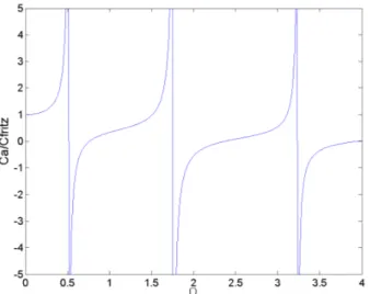
Ca= 1 Ω 1 D(Ω) ¡ J₁0(αΩ)Y1(Ω) −Y10(αΩ)J1(Ω) ¢ (33) Cν= 0 (34)

The added mass is displayed in Fig. 2 for α= 3. WhenΩ→ 0, it tends to the Fritz coefficient (Eqn. (22)). Equation (31) is invalid when the resonant condition D(Ωs) = 0 is satisfied.Ωsis

a non-dimensional resonance frequency defined byΩs=ωsR1/c

withωs the corresponding dimensional one. Practically, when

the frequency of the oscillation is close to a resonance frequency, the response amplitude of the fluid can be quite large even if the amplitude of inner cylinder is small. Figure 3 shows the curve which gives the smallest resonance frequency in function ofα. Following the methodology used in [35] for another problem, a solution of Eqn. (29) which satisfies the boundary conditions and the resonance condition can be found. Let us write a solution in the form: ˆ Φ= c cosθVm ω 1 D(ω)[E(ω,ω) sinωt − E(ωs,ωs) sinωst] with (35) E(ω1,ω2) = Y1 µ Ω1 r R1 ¶ J₁0(αΩ2) − J1 µ Ω1 r R1 ¶ Y₁0(αΩ2)

andΩidefined byΩi=ωR1/c (for i = 1, 2). ˆΦis a solution of

Eqn. (29). Equation (35) can be rewritten as: ˆ Φ= c cosθVm ω µ E(ω,ω)sinωt − sinωst D(ω) + sinωst E(ω,ω) − E(ωs,ω) D(ω) + sinωst E(ωs,ω) − E(ωs,ωs) D(ω) ¶ (36) Taking the limit ω→ωs and applying the Hopital’s rule to

Eqn. (36), give a resonant solution which satisfies the boundary conditions Eqn. (30):

Figure 3. VARIATION OF THE SMALLEST DIMENSIONLESS RESONANT FREQUENCY WITH THE CONFINEMENT RA-TIO. Φ= c cosθVm ω2 sZ(ωs) [ωst cosωst E (ωs,ωs) (37) +Ωs r R1 sinωst µ Y₁0 µ Ωs r R1 ¶ J₁0(αΩs) − J10 µ Ωs r R1 ¶ Y₁0(αΩs) ¶ + αωssinωst µ Y1 µ Ωs r R1 ¶ J₁00(αΩs) − J1 µ Ωs r R1 ¶ Y₁00(αΩs) ¶¸

where Z(ω) = dD(ω)/dω. The first term of the right-hand side is in proportion to t, so that the behavior of this resonant oscillation is mainly governed by the first term after a long time. When the amplitude become large, non-linearities in the Euler equations cannot be neglected any longer and the linear solution Eqn. (37) loses its validity. The corresponding fluid force takes the form of Eqn. (15) with: Ca= 1 ˆ Z(Ωs) (Y1(Ωs)J1(αΩs) − J1(Ωs)Y1(αΩs)) (38) Cν= ρπR 2 1ωs αΩs− (αΩs)−1 ωst ˆ Z(Ωs) ¡ Y1(Ωs)J10(αΩs) − J1(Ωs)Y10(αΩs) ¢ where: ˆ Z(Ωs) =Ωs · 1 −Ωs 1 −αΩs ¡ J1(Ωs)Y10(αΩs) −Y1(Ωs)J10(αΩs) ¢ − ¡J₁0(Ωs)Y1(αΩs) −Y10(Ωs)J1(αΩs) ¢¤ (39) A linearly time-dependent damping coefficient has appeared at the resonance frequency.

Lubricant film models

The challenge in lubricant film models is to include the tran-sient and the convective inertia terms. So as to make it analyti-cally possible, geometrical simplifications have to be made. By considering the triangle OO0A in Fig.1, the following relation is

obtained:

R2₁= (C + R1− h)2+ e2− 2(C + R1− h)e cosθ (40)

The above equation is a second order polynomial in h. So the solution of the problem of interest is easily found:

h = R1+C − e cosθ− R1

s

1 +C

2_{− e}2_sin2_θ

R2₁ (41)

In a lubricant film the radial clearance C and the motion ampli-tude e are very small compared to the radius of curvature R1:

C/R1<< 1 and e/R1<< 1 (42)

Then keeping only the first order terms in Eqn. (41), the film thickness is reduced to:

h(t) = C − e(t) cosθ (43) Moreover, since the film is very thin, the curvature effects are often neglected in the lubrification theory. This assumption allows the prescription of a Cartesian local coordinate system

(x = R1θ, y) on the plane of the lubricant film. x is in the

direc-tion of e_θand y in that of (−er) in Fig. 1. Denoting u and v the local fluid velocity along x and y, the Navier-Stokes equations for an infinitely long cylindrical film becomes:

ρ µ ∂u ∂t + u R1 ∂u ∂θ+ v ∂u ∂y ¶ = − 1 R1 ∂p ∂θ+ µ ∂2_u ∂y2 (44) ∂p ∂y = 0

with the mass conservation equation:

∂ρ ∂t + 1 R1 ∂u ∂θ+ ∂v ∂y= 0 (45)

Equation (44) is found by writing the Navier-Stokes equations in a dimensionless form and neglecting the terms of order (C/R1)2

and higher according to Eqn. (42). The boundary conditions can be written: u = 0, v = 0 at y = 0 (46) u = U, v =dh dt = ∂h ∂t + U R1 ∂h ∂θ at y = h(θ,t)

where U (θ,t) = − ˙e(t) sinθ. Integrating Eqn. (45) along the fluid thickness between 0 and h and using the Leibniz’s integration formula gives: ∂h ∂t + 1 R1 ∂h ¯u ∂θ = 0 (47)

where ¯u is the mean out-flow velocity at angleθ. Integrating the above equation between 0 andθand keeping in mind Eqn. (43) allow to obtain the expression of ¯u without the Navier-Stokes

equation:

¯

u(t,θ) = R1e(t) sin˙ θ

C − e(t) cosθ (48)

In order to continue the analytical derivation, particular velocity profiles along the fluid thickness satisfying the boundary condi-tions Eqn (46) and the mean out-flow velocity Eqn. (48) are often assumed. In [8,9], a parabolic profile is used and in [10,11] an

el-Figure 4. VARIATION OF Camin

CFritz AND

Cmax a

CFritz WITHεm.

liptical one. Once the corresponding u and v are determined, the pressure gradients are derived with the help of Eqn. (44) by using different approximation methods (momentum, energy or iterative method). The induced forces acting on the moving cylinder take the form:

F(t) = −¡ρπR2₁Ca(t) ¨e(t) +C1(t) ˙e(t) +C2(t) ˙e(t)2

¢

ex (49) which is the sum of an added mass, a viscous and a convec-tive inertia terms. The coefficients depend on the approximation methods and the assumed velocity profile. Since they vary with very similar tendencies in different papers [8,10,36,37], only the results for the energy method and parabolic velocity profile are shown here. For this case, the coefficients are given by:

Ca(t) = 12 5 1 α− 1 1 −p1 −ε(t)2 ε(t)2 (50) C1(t) = 12πµ 1 (α− 1)3 1 (1 −ε(t)2₎3/2 C2(t) =ρπR1 12 5 1 α− 1 1 ε(t)2 Ã 2 −ε(t)2 2p1 −ε(t)2− 1 !

These coefficients are function of the instantaneous time-dependent eccentricity ratio. For an harmonic movement, the coefficients oscillate between a maximum and a minimum value. These value for the added mass coefficients are:

C_amin=6 5 1 α− 1 (51) C_amax =12 5 1 α− 1 1 −p1 −ε2 m ε2 m (52) At a givenεm, the added mass coefficient oscillates between these

two values. The variations of Cmina

CFritz and

Cmax a

CFritz withεmare shown

in Fig. 4 forα= 1.01. Even with small displacements relative to radial clearance (ε→ 0), it shows that the incompressible invis-cid model underestimates the added mass in squeeze film flow. The difference is all the more pronounced as the confinement is high: C_amin CFritz =6 5 α+ 1 α2_{+ 1} α→1 7−→ 1.2 (53)

Figure 4 also shows that when the displacement of the inner cylinder is increased regarding the radial clearance, the maxi-mum added mass experienced by the solid can be more than two times higher than those predicted by Fritz during an oscillation. Moreover when an elliptical velocity profile is assumed, the un-steady inertia force are roughly 1.1 to 1.2 times bigger than those presented here with the parabolic profile, and an elliptical profile is expected to better describe the effects due to large amplitude cylinder motions [10, 11].

LIMITS AND CHALLENGES Comments on added mass

As written by Sarpaya (2004) [38], ”added mass is one of the best known, least understood, and most confused character-istics of fluid dynamics. It exists in all flows about bluff bod-ies. However, it manifests its existence, like all masses, only when it is accelerated”. Equation (10) suggests that the fluid force can be decomposed into an inviscid inertia term and a vorticity-dependent term. However the inertia term must not be confused with the added mass. Firstly, as shown in simplified viscous models, the added mass is influenced by the viscosity, see Eqn. (26) and Eqn. (27), so that the value obtained with inviscid models can only give an idea of the added mass value. Secondly, the vorticity-dependent term contains also a part in phase with the body acceleration, therefore which must be included in the added mass. In order to be convinced, the derivation in [39] is of particular interest. A body started from rest in a fluid initially at rest is considered. During an infinitively small∆t the vorticity

produced by the incremental velocity of the cylinder is contained in a small layer δ. Using the polar coordinates (r,θ) measured

from the direction of acceleration ex, Eqn. (10) can be rewritten:

F(t) = µ ρd dt Z _2π 0

I(t,θ,δ) sinθdθ+ρπR2₁e(t)¨

¶ ex (54) with I(t,θ,δ) = Z _R 1+δ R1 −r2_ω z(t,θ)dr

whereωzis the vertical component of the vorticity, so that: I(t,θ,δ) = Z _R 1+δ R1 −r2∂uθ ∂r − ruθ+ r ∂ur ∂θdr (55)

The conditions on the body and at the edge of the singular vor-ticity layer can be expressed by:

u(t, R1,θ) = ˙e(t) cosθer− ˙e(t) sinθeθ (56)

(a)

(b)

(c)

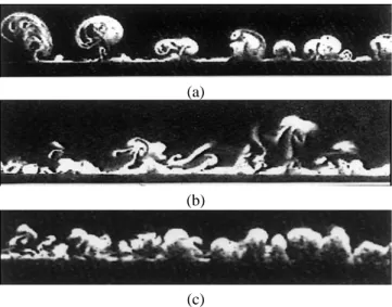
Figure 5. (a) HONJI-TYPE COHERENT STRUCTURES ATβ= 74800 ANDKC = 0.35ON THE HALL-LINE, (b) QUASI-COHERENT STRUC-TURES IN ZONE D AT β = 1365000AND KC = 0.3 (1.8KCcr),

(c) HTCS AND QCS IN ZONE C AT β= 1365000AND KC = 0.1

(0.59KCcr). REPRINT FROM SARPKAYA [27]

By integrating by part the first term in the integral in Eqn. (55), considering the above boundary conditions and taking the limit

δ→ 0, it comes: lim δ→0I(θ,δ) = limδ→0 £ −r2_u θ¤R_R1₁+δ= −2 ˙e(t)R21sinθ (58)

By introducing it in Eqn. (54), the fluid force is evaluated as:

F(t) =¡−2ρπR2₁e(t) +¨ ρπR2₁e(t)¨ ¢ex= −ρπR21e(t) e¨ x (59) which is the ideal inviscid value for an infinite fluid domain. It has been shown that if the body is started from rest in a viscous fluid initially at rest, the initial value of the added mass is in agreement with its ideal value (obtained with the potential the-ory) because the vorticity is still confined to a thin sheet on the boundary. In general, the diffusion has not the time to adjust to the unsteady conditions imposed on the flow, and the instanta-neous state is strongly influenced by the entire history of motion. In harmonic laminar unseparated movement, this results in the creation of a damping term, and in laminar linear movement with a general time-dependency, this can be expressed by a convolu-tion product [40]. In cases in which no wake is formed, and at sufficiently high Stokes number so that the boundary layer is very thin, this derivation can help to explain why the ideal added mass for an infinite fluid domain is a good fluid forces approximation.

Stability of the two-dimensional flow

When the inner cylinder rotates at a given frequency and the outer one is at rest, the two-dimensional fluid flow is known to be unstable to a three-dimensional centrifugal instability, result-ing in the formation of the Taylor vortices. In the case

consid-Figure 6. ZONES IN THE PARAMETERS SPACE (KC,β).

ered in this paper, the inner cylinder is not subjected to a rotat-ing motion, but is subjected to a radial oscillation. No result on the stability of this flow is available in the literature for a con-fined fluid domain. However, more is known for the case of a circular cylinder oscillating in an infinite fluid domain. The instability, which was first discovered by Honji (1981) [41], re-sults in a well-organized ”disturbed laminar” regime which has three-dimensional features. This fluid flow consists in a series of mushroom-shape vortex structures (see Fig. (5.a)) along the two lines where the local ambient velocity is maximum (at the crown of the cylinder). They are named ”Honji-type coherent struc-tures, HTCS” in [21, 42]. This regime clearly provides a limit on the range of validity of the Stokes-Wang theory, which assumes a two-dimensional flow. Hall [43] carried out a stability analysis of the two-dimensional flow assuming a largeβ. His study shows that these coherent structures (of centrifugal nature) appear when the Keulegan-Carpenter number is equal to the critical value:

KCcr= 5.78β−1/4(1 + 0.21β−1/4+ ...) (60)

which is in accordance with Honji’s experiments. This equa-tion corresponds to the Hall-line in Fig. 6. When the Keulegan-Carpenter number exceeds this critical value (zone D), HTCS may first exhibit a disturbed form (see Fig. 5(b)) giving rise to ”Quasi-coherent structures, QCS” [21]. If KC is again increased, separation, vortex shedding and turbulence may appeared. Ir-regular boundary-layer type instabilities over a finite region of

KC smaller than KCcr(zone C) are also observed [21, 42]. They

consist of a combination of QCS and occasional HTCS (see Fig. 5(c)). The lower limit where no instabilities are created dur-ing an entire cycle is experimentally given by the stability line defined by:

KCs≈ 12.5β−2/5 (61)

Figure 6 displays the different zones separated by the Hall-line and the stability line. These three-dimensional structures can strongly influence fluid forces, and specially the fluid damping term. In some measurements obtained atβ= 1000 [5], HTCS

are linked to a jump in the drag coefficient from Cd (Eqn. (27))

for KC < KCcrto 1.3Cdwhen the structures appeared. In zones A

and B (Fig. 6), no instability is predicted so that the Stokes-Wang theory is expected to be valid. However, there is experimental evidence that it is only valid whenβ< 4500. When the Stokes number exceeds this value a jump from Cdto 2Cdis observed in

zones B and C in many experiments [21, 44, 45]. Whereas this jump could be explained by the existence of QCS in zone C, the reason why it also occurs in zone B, even for Keulegan-Carpenter number as much as two orders of magnitude below KCs, is still

missing. This indicates that the Hall-line and the stability line are not the only limits of the Stokes-Wang theory and that the flow may be subjected to another instability not yet identified, perhaps in other regions of the cylinder. As suggested in [45], it may be induced by structural changes in the boundary layer. It will be very difficult to identify the reason of this damping term jump. Since it occurs at high Stokes number and is a three-dimensional phenomenon, it is numerically very costly and even out of reach for the highest Stokes numbers. It is also difficult to appreciate experimentally since the boundary layer is all the thinner asβis high.

Due to the statistical nature of the structures, the different zones in Fig. 6 can not be separated by simple lines. For instance, the stability line comes from human interpretation of intermittent fluid motions [21]. Moreover, the lines depend not only on the dimensionless parameters KC andβbut also on more uncontrol-lable ones such as the presence of air bubbles in the fluid and on the cylinder, temperature gradients, dissymmetry in the base flow, roughness. There have been some experimental attempts to identify the roughness influence in this flow. In [44], the roughness induced by an abrasive paper characterized by a ratio

k/d = 0.00079 is considered. A jump in the damping coefficient

from 2C_d for a smooth surface to 3C_d with the abrasive paper was found. Some experiments in [21] carried out at k/d ≈ 0.01 have shown that the flow separates from the sand grains at all the parameter values performed in the ranges 104_<β_{< 1.3.10}6_and

0.0052 < KC < 0.6. These attempts to identified the roughness influence can not yet be industrially used since much more ex-periments and theoretical studies have to be performed so as to make it understandable.

CONCLUSION

Various fluid force models have been reviewed for an os-cillating infinitely long circular cylinder in cylindrical confine-ment and in infinite fluid domain. It has been shown that the in-compressible inviscid model provides a lower limit of the added mass term when the flow is unseparated. This added mass term is only slightly increased by viscous corrections, see Eqn. (26) and Eqn. (27) for a reasonable confinement, but is strongly underes-timated in extreme confinement (see Eqn. (51) and Fig. 4). It is also the lower limit in case of a compressible flow, when the os-cillation frequency is smaller than the resonance frequency (see

Eqn. (33) and Fig. 2). Moreover it does not predict any damp-ing terms, which are of considerable importance even if they are much smaller than the added mass term in norm. They can ef-fectively limit the body motions by absorbing a part of the exci-tation energy. Damping can arise from laminar viscous effects, see Eqn. (26) and Eqn. (27), but also from the flow induced by the body motion in lubricant film (Eqn. (50)). In infinite fluid domain, it has been shown that the damping term predicts by the Stokes-Wang theory is available only in a small part of the parameters space (KC,β) and strongly underestimates the real damping induced by three-dimensional instabilities in the other zones. So, the simplified models used in design office tend to un-derestimate both added mass and damping effects. Design mar-gin could be significantly improved by taking into account the real fluid behavior. However, a huge amount of experimental, theoretical and numerical studies is still to be done. For instance, there is nothing on the stability of the two-dimensional cylindri-cally confined flow induced by radial motions of the inner cylin-der.

REFERENCES

[1] Bouard, R., and Coutanceau, M., 1980. “The early stage of development of the wake behind an impulsively started cylinder for 40 < Re < 104”. J. Fluid Mech., 101, pp. 583– 607.

[2] Haller, G., 2004. “Exact theory of unsteady separation for two-dimensional flows”. J. Fluid Mech., 512, pp. 257–311. [3] Dutsch, H., Durst, F., Becker, S., and Lienhart, H., 1998. “Low-Reynolds-number flow around an oscillating circu-lar cylinder at low Keulegan-Carpenter numbers”. J. Fluid

Mech., 360, pp. 249–271.

[4] Tatsuno, M., and Bearman, P., 1990. “A visual study of the flow around an oscillating circular cylinder at low Keulegan-Carpenter numbers and low Stokes numbers”. J.

Fluid Mech., 211, pp. 157–182.

[5] Sarpkaya, T., 1986. “Force on a circular in viscous oscil-latory flow at low Keulegan-Carpenter numbers”. J. Fluid

Mech., 165, pp. 61–71.

[6] Williamson, C., 1985. “Sinusoidal flow relative to circular cylinders”. J. Fluid Mech., 155, pp. 141–174.

[7] Koumoutsakos, P., and Leonard, A., 1995. “High resolu-tion simularesolu-tions of the flow around an impulsively started circular cylinder using vortex methods”. J. Fluid Mech.,

296, pp. 1–38.

[8] El-Shafei, A., and Crandall, S., 1991. “Fluid inertia forces in squeeze film dampers”. ASME, Rotating Machinery and

Vehicule Dynamics, 35, pp. 219–228.

[9] Tichy, J., and Bou-Sa¨ıd, B., 1991. “Hydrodynamic lubrifi-cation and bearing behavior with impulsive loads”. STLE,

Trib. Trans., 34, pp. 505–512.

cylindrical squeeze films. part I: short and long lengths”. J.

Fluids Struct., 15, pp. 151–169.

[11] Usha, R., and Vimala, P., 2003. “Squeeze film force using an elliptical velocity profile”. ASME, J. Appl. Mech., 70, pp. 137–142.

[12] Vance, J., 1988. Rotordynamics of Turbomachinery. John Wiley and sons, New York.

[13] Sigrist, J.-F., 2004. “Mod´elisation et simulation num´erique d’un probl`eme coupl´e fluide/structure non-lin´eaire. Ap-plication au dimensionnement de structures nucl´eaires de propulsion navale”. PhD Thesis, University of Nantes, France.

[14] Sigrist, J.-F., Laine, C., Lemoine, D., and Peseux, B., 2003. “Choice and limits of a linear fluid model for the numeri-cal study in dynamic fluid structure interaction problem”. In Proceedings of ASME, Vol. 454 of Pressure Vessel and

Piping, Cleveland, pp. 87–93.

[15] Melot, V., Sigrist, J.-F., Laine, C., Auvity, B., and Peerhos-saini, H., 2005. “Fluid structure interaction for a strongly accelerated cylinder: a numerical study of flow and fluid forces”. In 11th International Topical Meeting on Nuclear Reactor Thermal Hydraulics, Avignon, France.

[16] Noca, F., Shiels, D., and Jeon, D., 1999. “A comparison of methods for evaluating time-dependent fluid dynamic forces on bodies, using only velocity fields and their deriva-tives”. J. Fluids Struct., 13, pp. 551–578.

[17] Quartapelle, L., and Napolitano, M., 1982. “Force and mo-ment in incompressible flows”. AIAA Journal., 21, pp. 911– 913.

[18] Saffman, P., 1993. Vortex Dynamics. Cambridge University Press, Cambridge.

[19] Keulegan, G., and Carpenter, L., 1958. “Forces on cylinders and plates in an oscillating fluid”. J. Res. Nat. Bur. Stand.,

60, pp. 423–440.

[20] Axisa, F., 2001. Mod´elisation des syst`emes m´ecaniques.

Int´eractions fluide/structure. Herm`es.

[21] Sarpkaya, T., 2001. “Hydrodynamic damping and quasi-coherent structures at large Stokes numbers”. J. Fluids Struct., 15, pp. 909–928.

[22] White, E., Rice, J., and Ergin, F., 2005. “Receptivity of sta-tionary transient disturbances to surface roughness”. Phys.

Fluids, 17, p. 064109.

[23] Bottaro, A., and Zebib, A., 1997. “G¨ortler vortices pro-moted by wall roughness”. Fluid Dyn. Res., 19, pp. 343– 362.

[24] Joseph, G. G., Zenit, R., Hunt, M. L., and Rosenwinkel, A. M., 2001. “Particle-wall collisions in a viscous fluid”. J.

Fluid Mech., 433, pp. 329–346.

[25] Protas, B., Styczek, A., and Nowakowski, A., 2000. “An effective approach to computation of forces in viscous in-compressible flows”. J. Comp. Phys., 159, pp. 231–245. [26] Tan, B., Thompson, M., and Hourigan, K., 2005.

“Evaluat-ing fluid forces on bluff bodies us“Evaluat-ing partial velocity data”.

J. Fluids Struct., 20, pp. 5–24.

[27] Morison, J., O’Brien, M., Johnson, J., and Schaaf, S., 1950. “The force exerted by surface waves on piles”. Petroleum

Transactions, AIME, 189, pp. 149–157.

[28] Sarpkaya, T., 2001. “On the force decompositions of Lighthill and Morison”. J. Fluids Struct., 15, pp. 227–233. [29] Fritz, R., 1972. “The effects of liquids on the dynamics motion of immersed solids”. Trans. ASME, J. Eng. Ind., pp. 163–171.

[30] Chen, S., Wambsganss, M., and Jendrzejczyk, J., 1976. “Added mass and damping of a vibrating rod in confined viscous fluids”. ASME, J. Appl. Mech., pp. 325–329. [31] Chen, S., 1987. Flow induced vibrations. Hemisphere

Pub-lishing Corporation.

[32] Sinyavaskii, V., Fedotovskii, V., and Kukhtin, A., 1980. “Oscillation of a cylinder in a viscous fluid”. Prikladnaya

Mekhanika, 16.

[33] Stokes, G., 1851. “On the effect of the internal friction of fuids on the motion of pendulums”. Trans. Camb. Phil.

Soc., 9, pp. 8–106.

[34] Wang, C., 1968. “On high-frequency oscillatory viscous flows”. J. Fluid Mech., 32, pp. 55–68.

[35] Kurihara, E., Inoue, Y., and Yano, T., 2005. “Nonlinear resonant oscillations and shock waves generated between two coaxial cylinders”. Fluid Dyn. Res., 36, pp. 45–60. [36] Lu, Y., and Rogers, R., 1995. “Instantaneous squeeze film

force between a heat exchanger tube with arbitrary tube mo-tion and a support plate”. J. Fluids Struct., 9, pp. 835–860. [37] Zhou, T., and Rogers, R., 1997. “Simulation of two-dimensional squeeze film and solid contact forces acting on a heat exchanger tube”. J. Sound. Vib., 203, pp. 621–639. [38] Sarpkaya, T., 2004. “A critical review of the intrinsic of

vortex-induced vibrations”. J. Fluids Struct., 19, pp. 389– 447.

[39] Leonard, A., and Roshko, A., 2001. “Aspects of flow-induced vibration”. J. Fluids Struct., 15, pp. 415–425. [40] Basset, A. B., 1888. “On the motion of a sphere in viscous

fluid”. Phil. Trans. Roy. Soc. Lond., 179, pp. 43–63. [41] Honji, H., 1981. “Streaked flow around an oscillating

cir-cular cylinder”. J. Fluid Mech., 107, pp. 507–520.

[42] Sarpkaya, T., 2002. “Experiments on the stability of sinu-soidal flow over a circular cylinder”. J. Fluid Mech., 457, pp. 157–180.

[43] Hall, P., 1983. “On the stability of unsteady boundary layer on a cylinder oscillating transversely in a viscous flow”. J.

Fluid Mech., 146, pp. 337–367.

[44] Chaplin, J., and Subbiah, K., 1998. “Hydrodynamic damp-ing of a cylinder in still water and in transverse current”.

Appl. Ocean Res., 20, pp. 251–259.

[45] Chaplin, J., 2000. “Hydrodynamic damping of a cylinder atβ= 106_{”. J. Fluids Struct., 14, pp. 1101–1117.}