A PDE viewpoint on basic properties of coordination algorithms with symmetries

A PDE viewpoint on basic properties of

coordination algorithms with symmetries

Alain Sarlette and Rodolphe Sepulchre

Abstract— Several recent control applications consider the

coordination of subsystems through local interaction. Often the interaction has a symmetry in state space, e.g. invariance with respect to a uniform translation of all subsystem values. The present paper shows that in presence of such symmetry, fundamental properties can be highlighted by viewing the distributed system as the discrete approximation of a partial differential equation. An important fact is that the symmetry on the state space differs from the popular spatial invariance property, which is not necessary for the present results. The relevance of the viewpoint is illustrated on two examples: (i) ill-conditioning of interaction matrices in coordination/consensus problems and (ii) the string instability issue.

I. INTRODUCTION

During the last decades, the control literature has consid-ered several applications involving the collective behavior of locally interacting subsystems. For instance, distributed con-trol is applied e.g. to stabilize a perfectly smooth configura-tion for a membrane or segmented telescope mirror (see [24], [13], [3]), or for cross-directional control of industrial paper machines (see [25], with additional applications); platoons of cars following each other are considered a key technology enabling automated highways (see [26]); the “consensus problem” where a set of communicating agents must reach agreement on a decision value has become standard (see [27] for an early discussion, [20] for a review).

Applications focus on different aspects like optimal con-figuration, collision avoidance, nonlinear dynamics,... in the literature on vehicle formation control (see e.g. [18], [17], [11], [7], [15]); information passing issues, e.g. time delays and the graph structure formed by communication links, in the consensus literature [27], [4], [21], [20]; decentralized linear controller design in the distributed systems literature (see e.g. [25], [13], [2]). These different studies feature similar basic properties for controlling the overall behavior of a set of locally interacting entities, e.g. phenomena due to very different system response to long-range and short-range effects (see e.g. [3], [24], [14], [8], [21], [16]).

The present paper proposes to view distributed systems with particular symmetries as the discretization of a partial differential equation (PDE); it shows that this allows to study fundamental system properties on the basis of the continuous PDE approximation. Specifically, the considered distributed systems consist of linear subsystems which are Department of Electrical Engineering and Computer Science (Mon-tefiore Institute, B28), University of Li`ege, 4000 Li`ege, Belgium.

alain.sarlette@ulg.ac.be, r.sepulchre@ulg.ac.be

locally coupled through an operator satisfying a state sym-metry condition. The coupling operator is then viewed as the

discretization of a spatial derivative operator. This approxi-mation is shown to be valid for long-range spatial signals. The utility of our viewpoint is illustrated by (i) providing a natural explanation for several observations associated to very different system response to long-range and short-range effects; (ii) showing that spatial invariance is not necessary for these observations to hold; and (iii) highlighting the link between string stability (see e.g. [22], [26]) and stability of the associated PDE for some simple settings.

The goal is to draw a link which allows to reflect on the behavior of locally coupled distributed systems by exploiting existing knowledge and tools for PDEs. The link between PDEs and their discretization is subtle; see e.g. the finite difference PDE discretization literature [19], [5], [9] which studies the converse operation: approximating a continuous PDE by a discrete system. Formal conclusions are therefore limited in this paper. The hope is that controller design can benefit from intuitive insights of the PDE viewpoint, although final analysis of the resulting system may still have to consider the exact discrete setting. It seems that this has not been exploited in the literature. The fact that PDEs in physics are often used to model the behavior of interacting particles supports our point.

A complementary approach may be found in papers like [12]: interactions on graphs are written with “partial difference equations” whose abstract formulations mimick PDEs; however, the only abstract analogy precludes intuitive comparison of system properties.

Much previous work on locally coupled distributed sys-tems focuses on spatially invariant syssys-tems. Analysis (see e.g. “spatial bandwidth” discussion in [14], [8], [1]) and constructive controller design results are proposed thanks to a “spatial frequency shaping” approach (see e.g. [25], [13], [2]), similar to the standard “temporal frequency shaping”. The present paper rather proposes a “spatial continuous” approximation of distributed systems, similar to the standard approximation of time sampled systems by continuous-time equations. It shows that spatial invariance is in fact not nec-essary for several observations, which is a major distinction with respect to previous work.

A behavorial viewpoint on interconnected systems and symmetries can be found e.g. in [10].

The paper is organized as follows. Section II defines how to associate a PDE to a discrete distributed system satisfying certain properties. The following sections justify this step

by showing that the associated PDE reflects some basic properties of the distributed system. Section III considers the correspondence at a static level between local coupling and spatial derivatives; this allows to naturally explain how the collective response of a coupled system differs for long-range and for short-long-range effects. Section IV considers the link between dynamical distributed systems and associated PDEs, starting with examples of the string stability problem before briefly discussing the general case; the latter is the subject of ongoing investigation.

Notation: Imaginary unit is j = √−1; ksk and arg(s) denote the norm and angular argument of complex number s. R>0 is the set of strictly positive real numbers.

II. ASSOCIATING APDETO A DISTRIBUTED SYSTEM The present section takes the opposite step of PDE dis-cretization (see e.g. [19], [9], [5]). For simplicity, everything is kept one-dimensional at this stage.

Consider a distributed system composed ofN subsystems. Denote by u(k, t), y(k, t) and Hk respectively the scalar

input, scalar output and linear dynamics of subsystemk, for k = 1, 2, ..., N . Dynamics are typically formulated as

Pk(_dtd)y(k, t) = Qk(_dtd)u(k, t) (1)

where Pk(_dtd) and Qk(_dtd) are constant coefficient

polyno-mials in the time derivative operator. Denoting u(t) and y(t) the column vectors containing all u(k, t) and all y(k, t) respectively, the subsystems are coupled through

u(t) = Γy(t) (2)

whereΓ is a linear static operator represented by a constant matrix _{∈ R}N ×N; the element in row l, column k of Γ is denoted Γl,k. To separate spatial and temporal couplings,

we here assume identical subsystem dynamics Hk = Hj ∀j, k; future work might relax this condition. The following assumptions are considered on the coupling.

(A.1) Symmetry in _{y: ∃ M ≥ 1 such that (i) y(k) = k}m belongs to the kernel ofΓ, i.e.P_k Γl,kkm= 0 ∀l, for

all_{m ∈ {0, 1, ...M − 1}; (ii)}P_k Γl,kkM 6= 0.

(A.2) Local coupling (one-dimensional lattice): _{∃ c ≪ N} such thatΓk,k+m= 0 when |m modulo N| > c.

The meaning of (A.2) is clear; it can be easily adapted to multi-dimensional coupling lattices. The modulo N opera-tion allows ring interconnecopera-tions where the “last” subsys-tems are coupled to the “first” ones. Integer M in (A.1) characterizes the degree of state space symmetry, associated in what follows to the order of spatial derivatives. M = 1 corresponds toP_k Γl,k= 0 which implies that any constant

signaly(k) = y leads to u(k) = 0; this situation is familiar at least in consensus problems. Importantly, note that spatial invariance is not considered:Γ is not assumed to be circulant. Assumptions (A.1) and (A.2) often hold locally ink. Typ-ically, higher symmetry orderM is obtained when disregard-ing the boundary of the overall system, where the number of coupled subsystems decreases. Since the developments in this paper are based on spatially local analysis, they still very reasonably hold when discarding boundaries.

Proposition 1: Associate to the spatially discrete signal

y(k, t) the spatially continuous signal y(x, t), where x is continuous. If Γ satisfies (A.1), then a Taylor development of (1),(2) associates toy(x, t) the “infinite-order” PDE

P (_dtd)y(x, t) = Q(_dtd) +∞ X q=0 aq(x) (q+M)! ∂M+q ∂xM+q ! y(x, t) (3)

where aq(x) is a continuous interpolation of aq(k) = P

lΓk,l((l − k)moduloN)q+M. In particular, forx = k the PDE becomes equal to the distributed system equation.

Proof: One readily checks, by expanding the expression, that (A.1) is equivalent to P_l Γk,l(l − k)m= 0 ∀l for all m ∈ {0, 1, ...M − 1}. Consider the Taylor expansion

y(k + n) = y(k) + n_∂x∂y(k) + n2 1 2

∂2_y

∂x2 + ... (4) where constants in n are overlined for better visualization. Inserting (4) inu(k) =P_lΓ(k, l)y(l) with l = k + n, (A.1) implies that the _{M first terms of (4) sum to zero, ∀k; the} others yield coefficientsaq(k) as specified. Thus by taking aq(x) to be interpolations of the aq(k), (3) indeed becomes

equal to the distributed system equations forx = k. △

Remarks:

(a) The infinite series in (3) is not handy; its convergence for_{x 6= k is an issue that will not be discussed here.} The following sections show that some properties of the distributed system can be investigated by truncating the sum in (3) to a few terms. This kind of argument is well known in the finite differences literature like [19], [9]. The important property is the absence of spatial derivatives of orders_{0 to M − 1 implied by (A.1).} (b) The assumed invariance combines elements on the same

row of Γ, implying symmetry with respect to certain y-patterns. In contrast, spatial invariance ([8], [2],...) requires equality of elements on the same diagonal of Γ, such that Γ becomes circulant; this is a symmetry in k (or x). If (A.1) and spatial invariance hold, then (3) becomes a (infinite-series) linear PDE with constant coefficients aq, and spatiotemporal frequency domain

tools can be used. This is strictly analog to time-domain characterizations: time-invariance simplifies the analysis but many properties hold without it.

We believe that state space symmetry, as a fundamental

structural property of the coupling characterizing the

dis-tributed system, plays an important role regardless of the complexity of subsystem dynamics. Taking such structural properties into account in large state space approaches to analysis and design can be difficult. The following sections illustrate how the spatial derivative/PDE viewpoint, which inherently contains the symmetry, provides useful insight.

III. LOCAL COUPLING AS DISCRETIZED SPATIAL DERIVATIVES

This section leaves dynamics aside, focusing on the inter-pretation of coupling operatorΓ as a discretization of spatial derivatives. This is justified as follows.

Proposition 2: Consider a linear static coupling (2)

satisfy-ing (A.1) and (A.2). Then the small-q terms are dominant in the Taylor series of (3) describing Γ at least for low spatial frequencies of a harmonic signal y(k) = sin(ωk). In particular, the amplification ofy through Γ decreases as ωM _{whenω approaches 0.}

Proof: Considery(l) = y(k+n) = sin(ω(k+n)). Building its Taylor expansion around y(k) and applying (2) as for Proposition 1 leads to u(k) = +∞ X q=0 X l Γk,l(ω(l−k)) (q+M ) (q+M)! ! bq(k) (5)

where_|bq(k)| ∈ {sin(ωk), cos(ωk)} ≤ 1 ∀k, q. Low spatial

frequencies correspond to ω = f π_N with f a small integer. If Γk,l 6= 0, then (A.2) implies |(l − k)| ≤ c ≪ N so ω(l − k) ≪ 1. Therefore the series is dominated by the terms of smallq. In particular, the first nonzero term implies

a behavior inωM _{when ω tends to 0. △}

Remarks:

(a) The conditions “small_{ω” and “local coupling c ≪ N”} are actually combined to get _{ωc ≪ N. Thus for more} localized coupling (smallerc), the approximation holds up to higher frequenciesω.

(b) If the moduloN operation is used in (A.2), then the distributed system is coupled in a ring structure and the continuous variablex belongs to the circle S1_{. If (A.2)}

holds without applyingmoduloN , then x belongs to a line segment [x0, xL].

The viewpoint of Γ as a discretized spatial derivative provides a natural fundamental explanation for an order of magnitude difference in responses to long-range and to short-range effects in distributed systems. Phenomena related to the latter fact — e.g. bad system conditioning for robust-ness/performance (see [3], [24], [14], [8]), or slow consensus in non-“small-world” networks (see [21], [16] and references therein) — have been independently observed in several applications. The following reviews several examples with our common viewpoint. Spatial invariance plays an important role in existing studies, like [1]. However, according to the present interpretation, spatial invariance is not necessary for the observations to hold; this is illustrated in Example 4.

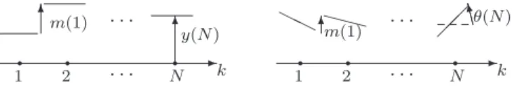
Example 1: (see Figure 1, e.g. [3]) A segmented mirror

is composed of straight segments aligned along a spatial dimension at k = 1, 2, ..., N . The output m(k) used to control mirror shape is the difference in vertical position at adjacent segment edges. First assume that segments only translate vertically to positions y(k); then m(k) = y(k + 1) − y(k). Observability is seen to go down for long-range deformations; this induces noise robustness and performance issues in the MIMO controller design for the full system. This property can be understood by viewing outputs m(k) as the first-order spatial derivative (see Appendix) of states y(k): then m(k) is expected to linearly decrease to zero with spatial frequencyω.

A similar effect is observed for short-range deformations when segments only rotate to orientationsθ(k). In this case m(k) = − sin(θ(k + 1)) − sin(θ(k)) ≈ −(θ(k + 1) + θ(k)). Change of variables [¯θ(k), ¯m(k)] := (−1)k[θ(k), m(k)] transforms high spatial frequencyθ-signals into low spatial frequency ¯θ-signals and conversely, and leads to the same output equation as for vertical translation, m(k) = ¯¯ θ(k + 1) − ¯θ(k). The property is then similarly interpreted.

-k . . . . . . q q q 1 2 N 6_{m(1) 6} y(N ) -k . . . . . . q q q 1 2 N HH XX_6m(1) CCOθ(N )

Fig. 1. Setting of the segmented mirror example: (left) restricted to translation, (right) restricted to rotation.

Example 2: (see Figure 2, e.g. [24], [8]) A membrane is

controlled with actuators uniformly distributed at positions k = 0, 1, ..., N − 1. Actuator input y(k) is assumed to linearly induce deformations in its neighborhood, e.g. such that membrane displacementd(k) = y(k) + y(k−1)+y(k+1)₂ (except at boundaries). Controllability is seen to go down when approaching the spatial Nyquist frequency of short-range deformations. Change of variables [¯y(k), ¯d(k)] := (−1)k_{[y(k), −d(k)] brings the Nyquist frequency to the}

origin, transforming high spatial frequency[y, d]-signals into low spatial frequency [¯y, ¯d]-signals. The resulting equation

¯

d(k) = y(k−1)+¯¯ ₂y(k+1)− ¯y(k) involves a discretized second-order spatial derivative (see Appendix). This naturally ex-plains quadratic decrease of controllability for low frequency

¯

d-signals, thus for d-signals close to the Nyquist frequency.

-k 6 6 6 6 . . . . . . 6 6 6 1 2 3 N -k . . . . . . q q q q q q q 6 d(3) 1 2 3 N 0

Fig. 2. Setting of the membrane example: (left) actuator forces, here

y(k) 6= 0 for k = 3 only; (right) membrane response to these forces.

Example 3: (see e.g. [16]) The consensus problem requires

a set of agents, indexed byk, to reach agreement on an e.g. scalar quantity y. In the standard consensus algorithm (see e.g. [27], [20]), every agent moves towards the average of its “neighbors” in the “interconnection graph”:y(k)+_{= u(k) =} P

j∈neighbors(y(j) − y(k)) where y+ denotes the update on y. Particular graphs of interest are the path or the ring. In a directed ring,_{u(k) = y((k + 1)moduloN ) − y(k) ∀k. In} an undirected ring,_{u(k) = (y((k + 1)moduloN ) − y(k)) +} (y((k − 1)moduloN) − y(k)). The right sides of these equa-tions match coupling relaequa-tions of Example 1 and Example 2 respectively. The viewpoint of spatial derivatives explains why convergence speed to consensus decreases respectively asω and as ω2 _{for low spatial frequency disagreements.}

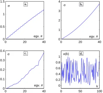
Example 4: Previous examples are all invariant in the

direction ofk, i.e. the output at k + 1 due to input at j + 1 is the same as the output at k due to input at j (up to possible boundary effects). This spatial invariance is broken

e.g. by introducing a k-dependent weight α(k) > 0 in the consensus algorithm on a directed ring:u(k) = α(k)(y((k + 1)moduloN ) − y(k)). Then u = Γy with Γ containing zeros except Γk,k = −α(k) and Γk,(k+1)moduloN = α(k), ∀k. Figure 3 shows the 40 smallest singular values σ of Γ for N = 100 and three different choices of α(k): uniform α(k) = 1 ∀k, linearly increasing α(k) = k/10, and uniformly independently randomly distributed in(0, 1). Only the first case is invariant along k, but the roughly linear decrease of singular values to zero, causing a decrease in consensus convergence speed, is clearly visible in all plots.

0 20 40 0 0.5 1 1.5 egv. # σ 0 20 40 0 1 2 3 4 egv. # σ 0 20 40 0 0.1 0.2 0.3 0.4 egv. # σ 0 50 100 0 0.2 0.4 0.6 0.8 1 k α(k) a. b. c. d.

Fig. 3. Smallest singular values of update coupling matrixΓ for consensus

in a directed ring with weightα(k): a. α(k) = 1 ∀k, b. α(k) = k/10 and

c.α(k) uniformly randomly chosen in (0, 1)N_{; plot d. shows the actual}

α(k) used in c.

IV. LINKING DISTRIBUTED SYSTEM ANDPDE PROPERTIES

Section III indicates that, for low spatial frequencies, the series development of Γ can be truncated to its first term(s). The present section returns to the interplay between spatial coupling and temporal dynamics in relation with the associated continuous limit of a partial differential equation. It first considers examples of the string stability problem before discussing the general case.

A. A PDE viewpoint on string stability

Consider N vehicles aligned one behind the other on a straight line (“the road”). The goal is to make each vehicle interact with neighboring vehicles to maintain inter-vehicle distance δ, see Figure 4. Numbering the vehicles from 1 (leader) to N (tail), the desired evolution of vehicle k’s position is _{p(k, t) = a(t) − δk for some a(t) : R →} R independent of k. The vehicles do not get an explicit referencea(t): to position itself correctly, vehicle k compares p(k) to e.g. p(k − 1) + δ. Define y(k, t) = p(k, t) + δk. Then the desired evolution becomes y(k, t) = a(t), i.e.

consensus of they(k), and vehicle k compares y(k) to e.g. y(k − 1). String stability — see e.g. [22], [6], [26] and references therein — characterizes how a disturbance on one vehicle affects the others: letting N tend to infinity, if a bounded disturbance ony(k) leads to unbounded disturbance on _{y(l) for |l − k| tending to infinity, then the system is}

string unstable; else it is string stable. Several dynamics and

coupling schemes have been analyzed against string stability. The following considers three simple examples.

e e e e e δ . . . . . . _{3 2 1 k ∼ x} -p

Fig. 4. Vehicles (depicted by circles) following each other on a straight road, to be examined for string stability. Note thatx increases in opposite

direction ofp.

Example 5: Vehicles have first-order dynamics and react to

the preceding vehicle according to

d

dty(k,t)= α (y(k−1,t)− y(k,t)) (6)

with_{α ∈ R}>0. Equation (6) is equivalent to the

continuous-time consensus algorithm on a directed path, which is known to appropriately converge. The cascade interaction structure implies that a disturbance onk is transmitted to k + 1, then k + 2,... through the vehicle chain. The transfer function at k from input_{y(k − 1) to output y(k) is s+α}α , so from y(k) to y(k + K), K > 0, it is ( α

s+α)

K_{. Its amplitude is lower than} 1 for any s = jω, tending to 1 for ω = 0. Thus time-varying disturbances are attenuated when transmitted through the chain, while a constant displacement of one vehicle implies the exact same displacement of its followers. The system is string stable.

In terms of the associated PDE, keeping the first term in the series, (6) corresponds to the transport equation

∂y ∂t = −α

∂y

∂x. (7)

Its solution is _{y = f (x − αt) for any function f: any} disturbance travels towards the positivex at speed α without modifying its shape. This situation is marginally stable. Adding the second term of the expansion yields

∂y ∂t = −α ∂y ∂x+ α ′ ∂2y ∂x2 (8) with α′ _{∈ R}

>0. This adds dissipation to (7), such that

disturbances are in fact smoothed out in time. More formally, assume a solutiony(x, t) = ejξx_est _{withξ ∈ R and s ∈ C.}

Plugging into (8) we obtain_{s = −jαξ − α}′ξ2_{. Thus s has}

negative real part, such that any solution that is not constant inx vanishes to zero as time evolves.

Example 6: Each vehicle follows the preceding one

accord-ing to second-order spraccord-ing-damper dynamics

d2

dt2y(k,t)= α (y(k−1,t)− y(k,t)) + β (_dtdy(k−1,t)−_dtdy(k,t))

(9) with _{α, β ∈ R}>0. Equation (9) is equivalent to a

for which convergence is not ensured as with first-order dynamics, see [23]. The transfer function from input_y(k−1) to outputy(k) is _s2βs+α_+βs+α. Its amplitude is larger than 1 at least for small s = jω, so slow disturbances are amplified along the chain and the system is string unstable. This conclusion still holds when adding dissipation _−γdtdy(k, t) withγ small enough.

In terms of the associated PDE, (9) corresponds to

∂2_y ∂t2 = −α ∂y ∂x− β ∂2_y ∂x∂t. (10)

Assuming a solution y(x, t) = ejξx_est_{, (10) requires s}2 ₌ −jαξ − jβξs. This implies s = −jλ1 ± λ2ejλ3 where λ1 = βξ₂ > 0, λ2 = √ kβ2_ξ2_+j4αξk 2 > 0 and λ3 = arg(β2_ξ2_+j4αξ)+π 2 ∈ ( π 2, 3π

4 ). Therefore one solution takes

the form s = µ1 − jµ2 with µ1, µ2 ∈ R>0, implying y(x, t) = ej(ξx−µ2t)_eµ1t_{: a solution propagating towards} positivex (the direction of information passing in the original discrete setting) is amplified as time evolves.

Example 7: Each vehicle is coupled to the preceding and

following one according to spring-damper dynamics: d2 dt2y(k,t) = α (y(k−1,t)+ y(k+1,t)− 2y(k,t)) (11) +β (d dty(k−1,t)+ d dty(k+1,t)− 2 d dty(k,t))

with_{α, β ∈ R}>0. Since the system is bidirectionally coupled,

it is not possible anymore to use the transfer function argument. Equation (11) is equivalent to a second-order dynamics consensus algorithm on an undirected graph, for which convergence can be ensured, see [23]. The system is string stable.

In terms of the associated PDE, (9) corresponds to

∂2_y ∂t2 = α ∂2_y ∂x2 + β ∂3_y ∂x2_∂t. (12)

For β = 0 this would be a wave equation; β > 0 adds dissipation, such that (12) is sometimes called the

strongly damped wave equation. Assumingy(x, t) = ejξx_est

with (12) requires s2 _{= −αξ}2 _{− βξ}2_{s; this implies s =} −βξ2_±√_β2_ξ4_−4αξ2

2 . Both cases have negative real part for all ξ. Thus any such solution vanishes to zero as time evolves andy(x, t) converges to a solution constant in x.

Remarks:

(a) Although the formal definition of string stability in-volves a spatially invariant system, observations remain valid if e.g. _{α, β depend on k (⇔ x); however, when} non-standard PDEs appear in this way, the required analysis may be difficult.

(b) The converging algorithms still feature different attenu-ation for short- and long-range disturbances, according to the observation of Section III. This is reflected in the ξ-dependence of the exponential attenuation factor. B. Discussion towards general conclusions

The previous examples are encouraging for a charac-terization of distributed system properties on basis of the associated PDE. However, the link is weak in the general case. A formal result takes the following form.

Proposition 3: Consider the PDE associated as in Section II

to a distributed system satisfying (A.1) and (A.2), truncated to a few first terms. If its general solution, restricted to propagation directions allowed by the distributed system (see e.g. Example 6), is exponentially unstable for all spatial frequencies in [0, ε) for some ε > 0, then the distributed system is unstable.

Proof idea: For low spatial frequencies _{∈ [0, ε), the} dis-tributed system described by the truncated PDE corresponds to (1) with modified couplingu(t) = (Γ + δ(t))y(t), where the elements ofδ become arbitrarily small when ε tends to 0. Robustness of exponential system properties then implies that the original distributed system is unstable. △

Remark: The truncation to “a few first terms” is chosen

to at least contain the first term which leads to exponential stability or instability of the PDE (e.g. second term for Example 5, first term for Examples 6 and 7). Adding further terms to this dominant part will not change the limit behavior for spatial frequency tending to0.

A tighter link cannot be proposed in general because the PDE approximation is valid for low spatial frequencies only: instability of the PDE at high spatial frequencies does not necessarily carry over to the distributed system, and instabil-ity of a distributed system at high spatial frequencies is not necessarily reflected on the PDE. The last point means that a stable PDE does not necessarily imply a stable distributed system. The existence of differences in stability properties between a PDE and its discretization is well-known and analyzed in the literature on finite differences for PDE numerical simulation, e.g. [19], [9]. Their results may be advantageously used in the present context both for analysis and design. Indeed, “bad” and “good” discretization schemes — the latter accurately reflecting stability properties of the original PDE — are characterized for many standard PDEs. It is worth noting that “good” space and time discretization schemes sometimes require implicit update equations.

In a design context, a first step would be to examine what type of PDE can be obtained with the imposed temporal dynamics and coupling structure of the distributed system. A second step could then design a PDE with the appropriate behavior on the basis of physical PDE knowledge. Further or in parallel, one might check how/if the distributed system can implement a “good” discretization of the designed PDE. The resulting discrete system could finally be analyzed on its own to confirm its behavior. The examples of Subsection IV.A, where PDE and distributed system have the same stability properties, are encouraging for our ongoing work on this subject.

V. CONCLUSION

The present paper proposes to study distributed systems with appropriate symmetries on the basis of an associated PDE. It illustrates this viewpoint by providing a natural inter-pretation for very different system response to long-range and short-range effects, and by highlighting the correspondence

between string stability of a discrete chain and stability of the corresponding PDE for several simple settings. The paper also shows that invariance along the “spatial” dimension along which the systems are interconnected is not necessary for fundamental observations to hold.

The goal of the paper is mainly to describe the concept and argue its plausibility. Several questions remain to be answered to formalize the link between PDE and distributed system behaviors. In particular, sufficient conditions ensuring stability of the distributed system (for all spatial frequencies) on the basis of conditions on the associated PDE would be of practical interest. Extensions are also planned to more complex dynamic settings — maybe nonlinear and heterogeneous subsystems — and higher-dimensional local coupling lattices; indeed [1] shows, under spatial invariance, that performance of locally coupled systems is inherently limited for 1- or 2-dimensional interconnection lattices, but better performance is recovered in higher dimensions. Most importantly, we plan to further examine distributed controller and algorithm design on the basis of associated PDEs. This could motivate further development of “PDE shaping con-trol”, where in contrast to traditional e.g. boundary control problems, the actual form of the PDE must be designed.

VI. ACKNOWLEDGMENTS

This paper presents research results of the Belgian Network DYSCO (Dynamical Systems, Control, and Optimization), funded by the Interuniversity Attraction Poles Program, initiated by the Belgian State, Science Policy Office. The scientific responsibility rests with its authors. The first author is supported as an FNRS fellow (Belgian Fund for Scientific Research).

REFERENCES

[1] B. Bamieh, M. Jovanovic, P. Mitra, and S. Patterson. Effect of topological dimension on rigidity of vehicle formations: fundamental limitations of local feedback. Proc. 48th IEEE Conf. Decision and

Control, pages 369–374, 2008.

[2] B. Bamieh, F. Paganini, and M.A. Dahleh. Distributed control of spa-tially invariant systems. IEEE Trans. Automatic Control, 47(7):1091– 1107, 2002.

[3] Ch. Bastin, A. Sarlette, R. Sepulchre, M. Dimmler, T. Erm, B. Bauvir, and B. Sedghi. European extremely large telescope M1 control strategies study. ESO Internal report E-TRE-ULG-0449-0007, 2009. [4] S. Boyd, A. Ghosh, B. Prabhakar, and D. Shah. Randomized

gossip algorithms. IEEE Trans. Information Theory (Special issue), 52(6):2508–2530, 2006.

[5] R.W. Brockett and J.L. Willems. Discretized partial differential equa-tions: Examples of control systems defined on modules. Automatica, 10(5):507–515, 1974.

[6] Kai Chung Chu. Decentralized control of high speed vehicle strings.

Transportation Research, pages 361–383, June 1974.

[7] J.P. Desai, J.P. Ostrowski, and V. Kumar. Modeling and control of formations of nonholonomic mobile robots. IEEE Trans. Robotics

and Automation, 17(6):905–908, 2001.

[8] S.R. Duncan and G.F. Bryant. The spatial bandwidth of cross-directional control systems for web processes. Automatica, 33(2):139– 153, 1997.

[9] J.A. Essers. Partial differential equations: characterization for numer-ical solution and the finite differences method. Master degree course

at Florida State University / University of Li`ege, 1988 / 2004.

[10] F. Fagnani and J.C. Willems. Interconnections and symmetries of linear differential systems. Mathematics of Control, Signals and Systems, 7(2):167–186, 1994.

[11] J. Fax and R.M. Murray. Information flow and cooperative control of vehicle formations. IEEE Trans. Automatic Control, 49(9):1465–1476, 2004.

[12] L. Galbusera, M.P.E. Marciandi, P. Bolzern, and G. Ferrari-Trecate. Control schemes based on the wave equation for consensus in multi-agent systems with double-integrator dynamics. Proc. 46th IEEE Conf.

Decision and Control, pages 1498–1503, 2007.

[13] D.M. Gorinevsky, S.P. Boyd, and G. Stein. Design of low-bandwidth spatially ditributed feedback. IEEE Trans. Automatic Control,

53(2):257–272, 2008.

[14] W.P. Heath. Orthogonal functions for cross-directional control of web forming processes. Automatica, 32(2):183–198, 1996.

[15] J.M. Hendrickx, B.D.O. Anderson, J.C. Delvenne, and V.D. Blon-del. Directed graphs for the analysis of rigidity and persistence in autonomous agents systems. International journal of robust and

nonlinear control, 17(10):960–981, 2007.

[16] J.H. Kim, M. West, S. Lall, E. Scholte, and A. Banaszuk. Stochastic multiscale approaches to consensus problems. Proc. 48th IEEE Conf.

Decision and Control, pages 5551–5557, 2008.

[17] J.R. Lawton and R.W. Beard. Synchronized multiple spacecraft rotations. Automatica, 38:1359–1364, 2002.

[18] N.E. Leonard, D. Paley, F. Lekien, R. Sepulchre, D. Frantantoni, and R. Davis. Collective motion, sensor networks and ocean sampling.

Proc. IEEE, 95(1):48–74, 2007.

[19] K.W. Morton and D.F. Mayers. Numerical solution of partial

differ-ential equations, an introduction. Cambridge University Press, 2005.

[20] R. Olfati-Saber, J.A. Fax, and R.M. Murray. Consensus and cooper-ation in networked multi-agent systems. Proc. IEEE, 95(1):215–233, 2007.

[21] A. Olshevsky and J.N. Tsitsiklis. Convergence rates in distributed consensus and averaging. Proc. 45th IEEE Conf. Decision and Control, pages 3387–3392, 2006.

[22] L. Peppard. String stability of relative-motion PID vehicle control.

IEEE Trans. Automatic Control, 19(5):579–581, 1974.

[23] Wei Ren and R.W. Beard. Distributed Consensus in Multi-vehicle

Cooperative Control. Communications and Control Engineering. Springer, 2008.

[24] G. Stein and D.M. Gorinevsky. Design of surface shape control for large two-dimensional arrays. IEEE Trans. Control Systems Technology, 13:422–433, 2005.

[25] G.E. Stewart, D.M. Gorinevsky, and G.A. Dumont. Two-dimensional loop-shaping. Automatica, 39(5):779–792, 2003.

[26] D. Swaroop and J.K. Hedrick (advisor). String stability of intercon-nected systems: an application to platooning in automated highway systems. PhD Thesis, University of California Berkeley, 1994. [27] J.N. Tsitsiklis and M. Athans (advisor). Problems in decentralized

decision making and computation. PhD Thesis, MIT, 1984. APPENDIX

The present appendix recalls Fourier transforms of discrete derivative approximations, to illustrate how they closely approximate continuous derivatives at low frequencies.

1st order: The first derivativey(1)_{(x) :=} dy

dx of signal y(x) is approximated by y(1)_{(k) = y(k+1)−y(k). Then y}(1)

is the convolution of_{y with the signal der = [−1 1 0 ... 0].} In the Fourier domain dy(1) _{= y dbder, where for a signal y}

of (e.g. even) length/period N the functions are defined at frequencies ωk = k2π_N with k = −N₂ , −N₂ + 1, ..., N₂ − 1.

Then dder(ωk) = ejωk/22j sin(ω₂k). For small ωk, this is a

close approximation in frequency domain of the continuous derivative c_dxd = jω.

2nd order: The second derivative y(2)_{(x) :=} d2y dx2 of y(x) is approximated by y(2)_{(k) = y(k + 1) + y(k − 1) −} 2y(k). Then y(2) _{is the convolution of y with dder =} [1 − 2 1 0 ... 0]. In the Fourier domain, dy(2) _{= y dbdder}

with ddder(ωk) = −4 sin2(ω₂k), which for small ωk is a close