Science Arts & Métiers (SAM)
is an open access repository that collects the work of Arts et Métiers Institute of
Technology researchers and makes it freely available over the web where possible.
This is an author-deposited version published in:
https://sam.ensam.eu
Handle ID: .
http://hdl.handle.net/10985/20167
To cite this version :
Paul KERDRAON, Boris HOREL, Patrick BOT, Adrien LETOURNEUR, David LE TOUZÉ
-Development of a 6-DOF Dynamic Velocity Prediction Program for offshore racing yachts - Ocean
Engineering - Vol. 212, p.107668 - 2020
Ocean Engineering 212 (2020) 107668
0029-8018/© 2020 Elsevier Ltd. All rights reserved.
Contents lists available atScienceDirect
Ocean Engineering
journal homepage:www.elsevier.com/locate/oceaneng
Development of a 6-DOF Dynamic Velocity Prediction Program for offshore
racing yachts
Paul Kerdraon
a,b,∗, Boris Horel
b, Patrick Bot
c, Adrien Letourneur
a, David Le Touzé
b aVPLP Design, 18 Allée Loïc Caradec, 56000 Vannes, FrancebEcole Centrale Nantes, LHEEA Lab. (ECN and CNRS), 1 Rue de la Noë, 44300 Nantes, France cNaval Academy Research Institute - IRENAV CC600, 29240 Brest Cedex 9, France
A R T I C L E I N F O
Keywords:
Dynamic Velocity Prediction Program (DVPP) Sailing yacht Offshore trimaran System-based modeling Time-domain simulation Hydrofoil
A B S T R A C T
Thanks to high lift-to-drag ratios, hydrofoils are of great interest for high-speed vessels. Modern sailing yachts fitted with foils have thus reached impressively high speeds on the water. But this hydrodynamic efficiency is achieved at the expense of stability. Accurate tradeoffs are therefore needed to ensure both performance and safety. While usual Velocity Prediction Programs (VPPs) are inadequate to assess dynamic stability, the varying nature of the offshore racing environment further complicates the task.
Dynamic simulation in the time-domain is thus necessary to help architects assess their designs. This paper presents a system-based numerical tool which aims at predicting the dynamic behavior of offshore sailing yachts. A 6 degrees of freedom (DOF) algorithm is used, calculating loads as a superposition of several components (hull, appendage, sails). Part of them are computed at runtime while the others use pre-computed dataset, allowing a good compromise between efficiency and flexibility.
Three 6DOF simulations of an existing offshore trimaran (a maneuver, unsteady wind conditions and quartering seas) are presented. They underline the interest of dynamic studies, demonstrating how important the yacht state history is to the understanding of her instantaneous behavior and showing that dynamic simulations open a different field of optimization than VPPs.
1. Introduction
The need for dynamic simulation is growing in many fields of engineering, as it allows to test and compare prototypes and processes at much lower costs than actual full-scale tests. Naval architecture is no exception. Nowadays, it widely relies on Velocity Prediction Programs (VPPs) to help architects and engineers in the design process of sailing yachts. However VPPs have proved inadequate to optimize
all of the design parameters. Originally introduced byKerwin(1978),
VPPs are constrained non-linear steady state optimizers which, based on experimental, numerical or empirical data, enable boat settings optimization to derive the reachable speeds in given steady conditions. Unlike inshore yachts such as the AC45 or the AC75 where class rules limit the acceptable wind and waves conditions, offshore vessels may encounter rough sea and wind conditions with short characteristic time of evolution. In such unsteady environments, racing yachts may be compelled to sail at much lower speed than the steady state optimized values. Assessing the boat real performance and her ability to safely maintain high average speeds in varying conditions is therefore a key
∗ Corresponding author at: VPLP Design, 18 Allée Loïc Caradec, 56000 Vannes, France.
E-mail addresses: kerdraon@vannes.vplp.fr(P. Kerdraon),boris_horel@hotmail.fr(B. Horel),patrick.bot@ecole-navale.fr(P. Bot), letourneur@vannes.vplp.fr(A. Letourneur),david.letouze@ec-nantes.fr(D. Le Touzé).
measure of her racing efficiency and should be included in the design trade-offs.
In addition, recent years have seen a substantial growth of foiling technologies, leading to fully flying yachts and introducing specific stability issues with direct impact on average speed. A better knowledge of the dynamic response of flying yachts is paramount for safe and sustained offshore flight. Non-linear couplings between the different degrees of freedom further complicate the study and traditional VPPs have proven inadequate to handle these matters with the accuracy required for high performance sailing.
In this context, numerical tools enabling time-domain analysis and including unsteady environment – often called Dynamic Velocity Pre-diction Programs (DVPPs) – have become a major research topic. This paper is interested in such a simulation tool, handling variable wind and waves as well as mode transition between Archimedean and
fully flying conditions. Section2presents a literature review on yacht
dynamic simulation. The mathematical modeling is given in Section3.
https://doi.org/10.1016/j.oceaneng.2020.107668
Notations
� Wave amplitude [m]
� Added mass coefficients matrix [kg, kg m,
kg m2]
�∞ Infinite frequency added mass matrix [kg,
kg m, kg m2]
� Damping coefficients matrix [kg/s, kg m/s,
kg m2/s]
�∞ Infinite frequency damping matrix [kg/s,
kg m/s, kg m2/s]
� Yacht breadth [m]
C Yacht center of effort
� Appendage characteristic chord length [m]
�� Sail drag coefficient [–]
�� Sail lift coefficient [–]
�� Midship section coefficient [–]
� Yacht draft [m]
� � Froude number [–], � � = ̄�∕√��WL
� External linear forces vector [N]
�� Force component i [N, Nm]
|��| Diffraction force modulus [N/m, N]
�� Reduced frequency [–], ��= �∕� �
G Ship center of gravity
� Acceleration of gravity [m/s2]
� Yacht inertia matrix [kg, kg m, kg m2]
�� Controller proportional coefficient [◦/◦]
� Wave number [m−1], � = 2�∕�
�� Unsteady wind intensity factor for
compo-nent � [–]
� Impulse response function matrix [kg/s2,
kg m/s2, kg m2/s2]
��� Yacht pitch radius of inertia [m]
�WL Waterline length [m]
� Yacht mass [kg]
� External moments vector [Nm]
� Outgoing body’s normal unit vector
O Origin of the ship reference frame ��
�� Pressure of incoming waves [N/m2]
�0=
(
�0, �0, �0
)
Earth-fixed reference frame
��=(��, ��, ��) Ship-fixed reference frame
�Sails Total sail area [m2]
�� Yacht wetted area [m2]
� Appendage characteristic period of
oscilla-tions [s]
�� Controller derivative coefficient [s]
�� Unsteady wind period for component � [s]
̄
� Yacht mean speed [m/s]
Section4presents and analyzes three examples of dynamic simulation
performed with the developed numerical tool.
2. Sailing yacht dynamic simulation
The ability to simulate maneuvers and especially tacking has long
been the main subject of sailing dynamic studies (Masuyama et al.,
1995; Keuning et al., 2005;Gerhardt et al., 2009). In match racing, maneuvers are critical and simulations provide an efficient way for
designers as well as crew to improve the on-water results (Binns et al.,
� Yacht linear velocity vector [m/s]
��∕f low Apparent flow velocity vector at X [m/s]
����� Wave orbital velocity [m/s]
� Leeway angle [◦]
�� Rudder angle [◦]
� Pitch angle [◦]
� Wave length [m]
� Ship-waves relative heading [◦]
� Ship perturbation vector [m, rad]
�� Potential of incoming waves [m2/s]
� Heel angle [◦]
�� Diffraction force phase [rad]
� Water density [kg/m3]
�air Air density [kg/m3]
� Yaw angle [◦]
�� Autopilot target heading [◦]
� Frequency-domain variable [s−1]
Wave frequency [s−1]
�� Frequency of encounter [s−1]
� Yacht angular velocity vector [s−1]
∇ Displacement [m3]
AWA Apparent Wind Angle
AWS Apparent Wind Speed
CFD Computational Fluid Dynamics
DOF Degree(s) of Freedom
DSYHS Delft Systematic Yacht Hull Series
DVPP Dynamic Velocity Prediction Program
IMS International Measurement System
QST Quasi-Steady Theory
RANS Reynolds-averaged Navier–Stokes
RAO Response Amplitude Operator
TWA True Wind Angle
TWD True Wind Direction (relative to North)
TWS True Wind Speed
VPP Velocity Prediction Program
2008). As match racing competitions are generally run inshore,
shel-tered from the deep-water waves, and due to the complexity of waves effect, the first numerical tools considered flat water conditions. Most of
these works are based on the usual maneuvering approach (Abkowitz,
1964) in which loads are described using hydrodynamic derivatives: a
Taylor-series expansion of the forces with respect to all the involved pa-rameters (attitudes, sinkage, speed components). Such models allowed the study of the three or four degrees of freedom (DOFs) boat motion (surge, sway, yaw and sometimes roll). Nevertheless foiling greatly enhances the need to factor in the two other degrees of freedom as heave (flight height) and trim (appendages angles of attack) are now
at the core of boat stability (Heppel,2015). Full 6 degrees of freedom
modeling is therefore needed.
Introduction of time-domain studies in the design of racing yachts occurred for the victorious 26th America’s Cup challenger Stars and
Stripes (seeOliver et al.,1987) using a quasi-steady approach. Velocity Prediction Program results were combined with wind statistics and game theory to simulate match races between several candidates and isolate the best performing design. Based on the widely used steady
state models of the IMS VPP (Claughton,1999), the four degrees of
freedom program ofLarsson(1990) included a first account of wave
effects by computing added resistance through strip theory.Masuyama
et al.(1993,1995) developed a numerical tool based on hydrodynamic derivatives computed from tank tests and aerodynamic coefficients
Fig. 1. Developed simulation tool visualization window.
derived from wind tunnel measurements. Comparison of their 4 degrees of freedom results with full-scale measurements proved successful. In
the second paper,Masuyama et al.(1995) reported on the substantial
role of sails in roll damping and proposed a strip theory model
ig-noring three dimensional effects.Keuning et al. (2005) enlarged the
possibilities and modularity of such tools by introducing the use of Delft Systematic Yacht Hull Series (DSYHS) to compute the hydrody-namic coefficients. While comparison with full-scale tests showed good agreement, the weaknesses of the aerodynamic model (based on the IMS VPP) is nevertheless underlined by the authors.
To the author’s knowledge,Day et al.(2002) were the first to report
on a 6 degrees of freedom time-domain simulation tool. The program used the Delft Systematic Yacht Hull Series for the hydrodynamic loads and the IMS VPP quasi-steady approach for sail forces. Comparison with full-scale data showed good trends although the author underlined
some discrepancies. A few years later,Harris(2005) proposed another
numerical tool to simulate the upwind behavior of sailing yachts. Ma-neuvering loads were computed through a panel code, while radiation and diffraction loads were expressed from strip theory. A strip theory approach was also used for the aerodynamic loads.
On the other hand, constant improvements of computational power have opened the possibility to use CFD for time-domain simulation by directly coupling the RANS (Reynolds Averaged Navier–Stokes) flow
solvers with rigid body dynamic solvers (Jacquin et al., 2005; Roux
et al., 2008; Lindstrand Levin and Larsson, 2017). Such approaches enable great accuracy while eliminating the need for empirical data or numerical pre-computations. The use of CFD as numerical VPP was achieved and work is now undertaken to add unsteady environ-ment. Nevertheless, the computational time and costs of such tech-niques make them currently unavailable for naval architects when the comparison of several designs and configurations is needed.
System-based approaches, on the contrary, use empirical and theo-retical models, experimental results or pre-computed numerical data to derive the hydrodynamic and aerodynamic loads and model the
boat global behavior (Horel, 2016, 2019) with a computational
ef-ficiency that enables systematic studies, of appendages shapes and configurations for instance.
This paper presents therefore a system-based approach to the
time-domain simulation of sailing yachts (seeFig. 1). Due to the importance
of the sea state on offshore yachts performance, the model was built to account for wave loads and thus enables the improvement of the yacht response. Besides, to allow an accurate optimization of foiling yachts, the numerical tool handles motion in the six degrees of freedom. Unlike most of the cited papers, it has been chosen to handle maneuvering loads not by Taylor expansions or semi-empirical formula but using interpolated Computational Fluid Dynamics (CFD) data to increase accuracy. The numerical models are presented in the following section.
Fig. 2. Coordinate systems definition. � is the leeway angle.
3. Mathematical modeling
This section presents the models implemented in the simulation tool to compute the loads of each yacht component and derive the ship motion.
3.1. Dynamics
The developed numerical tool is based on the time-domain integra-tion of the 6 degrees of freedom rigid body mointegra-tion equaintegra-tions, derived from the conservation of linear and angular momentum in the non inertial ship-fixed reference frame:
⎧ ⎪ ⎨ ⎪ ⎩ �[�̇ + ̇� × �� + � × (� + � × ��)] = � � ̇�+ � �� × ̇�+ � × � � + � �� × (� × �) = � (1) where � and � are the ship linear and angular velocity vectors, and
̇
�, ̇� their time derivatives. �, � are the external forces and moments
acting on the yacht, and �, � her mass and inertia at the origin � of the ship reference frame. � is the body’s center of gravity.
Unlike conventional boats, sailing yachts loading conditions are generally asymmetric to increase the righting moment (water ballast, canting keel, equipment windward stacking). Therefore no assumption is made hereafter on the values of the products of inertia of � or on the transverse coordinate of ��.
The ship-fixed reference frame ��=
(
��, ��, ��)is defined with ��
positive direction forwards, �� to port and �� upwards (seeFig. 2).
Its orientation with respect to the earth-fixed inertial reference frame
�0 = (�0, �0, �0)is expressed using the usual gimbal angles �, �, �
(roll, pitch and yaw).
The rotation matrix from the ship-fixed reference frame ��to the
earth-fixed one �0 is given by:
��→�0= ⎡ ⎢ ⎢ ⎢ ⎣
cos � cos � cos � sin � sin � − sin � cos � cos � sin � cos � + sin � sin � sin � cos � sin � sin � sin � + cos � cos � sin � sin � cos � − cos � sin �
− sin � cos � sin � cos � cos �
⎤ ⎥ ⎥ ⎥ ⎦ (2)
Thus vectors ��expressed in the body reference frame are transformed
into the Earth fixed frame using �0=��→�0��. The angular velocity
vector � in ��are linked to the derivatives of the gimbal angles by the
following expression: ⎡
⎢ ⎢ ⎣
1 sin � tan � cos � tan �
0 cos � − sin �
0 sin �∕ cos � cos �∕ cos �
⎤ ⎥ ⎥ ⎦ �= ⎡ ⎢ ⎢ ⎣ ̇� ̇� ̇� ⎤ ⎥ ⎥ ⎦ (3)
which presents a singularity for � = ±�∕2. This is however not an issue in normal sailing conditions.
Several explicit numerical integration schemes with various orders are available as well as adaptive time-stepping methods, which enable computational time optimization. In practice, with a small enough time-step, we experienced that the choice of integration scheme had no – or very limited – impact on the result.
External loads are expressed as a superposition of all boat loaded components and can be divided in three main groups: hull loads (H), appendage loads (AP) and aerodynamic loads (AE):
�= �H+ �AP+ �AE+
∑
�,�∈{�, �� , ��}
��∕�+�0→���� (4)
with � the gravity vector. The three main components are detailed in
the following sections. ��∕�is the interaction term of component � over
component �. As in the majority of system-based models most of those interactions are neglected. However, depending on the setups chosen by the user in the pre-computation steps, some of them may be accounted
for, such as the interaction between hull and appendages’ forces �AP∕H
for instance.
3.2. Hull loads
Hydrodynamic loads on the hull can be split in low frequency (maneuvering) and high frequency (seakeeping: radiation and waves) loads.
3.2.1. Maneuvering loads
Instead of the usual hydrodynamic derivatives approach (Abkowitz,
1964) for the maneuvering forces, the dynamic simulation tool uses
polynomial response surfaces based on numerical viscous computations (RANS) which allow to decrease the computation burden. The response surfaces are built on steady-state calculations over an appropriate range of hull attitude, sinkage, leeway angle and speed, which are then the input variables to the polynomial fit. The computations are carried out in flat-water conditions, and the hydrostatic components of the loads are removed so that they are only accounted once, when integrating over the wetted surface due to the incoming wave field.
It enables a full modeling of the six components of the hydrody-namic loads on each hull, including dependency to the boat possible changes of attitude and displacement due to the effect of appendages.
3.2.2. Radiation force
The higher frequency loads are based on the classical distinction between radiation, diffraction and Froude–Krylov forces. The former considers damping and added mass effects due to radiated waves generated by ship oscillations at the free surface. They are computed in the frequency-domain using the Boundary Element Method (BEM)
code Aquaplus (Delhommeau,1987) developed at the Ecole Centrale
de Nantes. Transformation of these frequency-domain coefficients to
the time-domain is carried out through Cummins equation (Cummins,
1962) convolving the impulse response function � with the hull
veloc-ity: �RD= − � ( ∞, ̄�)̈� − �(∞, ̄�)̇� − ∫ � 0 �(�− �, ̄�)̇� (�) �� (5)
where �RDis the radiation force, �
(
∞, ̄�)and �(∞, ̄�)the added mass
and damping at infinite frequency and mean speed ̄� and � the ship
perturbation vector. � is given by the inverse Fourier transform of the frequency dependent damping component:
�(�, ̄�)= 2 � ∫ ∞ 0 [ �(�, ̄�)− �∞ (̄ �)]cos (��) �� (6)
with � the frequency-domain variable.
3.2.3. Wave loads
As this simulation model is concerned with offshore yachts, only deep water waves are considered. Diffraction loads are the first wave excitation force component. They originate in the reflection of the incident waves on the ship surface. Similarly, they are linearly modeled through the seakeeping code outputs, but directly using the frequency-domain expression : �DF= �|��|(��) cos ( ��− �� + ��(��) ) (7)
where �DFis the diffraction force,|��| and ��its modulus and phase, �
the ship abscissa along the wave propagation axis, � the wave number
and � its amplitude. ��is the frequency of encounter, which for linear
waves is given by:
��= � −�
2
��cos � (8)
with � the angle between the ship track and the wave propagation and
� the yacht speed.
Finally, Froude–Krylov force �FK gathers the loads of the incident
wave pressure field ��on the instantaneous ship wetted surface ��:
�FK= − ∬
��
��� �� (9)
where � is the outward unit normal vector to the body surface. ��is
expressed through potential flow theory of gravity waves:
��= −� [ ��� �� + 1 2 ( ���)2 ] (10)
with � the fluid density and ��the incident waves potential.
While computing Froude–Krylov force, a correction of the hydro-static loads is also performed to account for the deformation of the free surface.
3.3. Appendage loads
Appendage loads are in a first approach modeled using a Vortex
Lattice Method (VLM, see for instanceKatz and Plotkin, 2001) with
correction for viscous effects. This provides a numerically efficient way to compute the spanwise distribution of lift for lifting surfaces of any aspect ratio, dihedral and sweep. Assuming that the appendages are not located in the wake of one another, their interaction is currently neglected. Velocity induced by the yacht angular motion, wave velocity field and appendage trimming angles are accounted for by computing effective angles between the appendage and the incoming flow follow-ing the Quasi-Steady Theory (QST) approach to compute the apparent flow velocity vector:
��∕f low= � + � × � − ����� (11)
where � is the coordinate vector of the considered location and �����
is the wave orbital velocity vector. The Vortex Lattice Method provides the full 6 components load tensor of each appendages, also the forces and moments generated by the appendages are accounted for. Loads are computed for each appendage without assuming any symmetry in the setup, so that asymmetric attitudes are reflected in the computed forces and moments and that windward and leeward appendages can be tuned differently.
The reduced frequency ��provides an interesting measure of the
importance of dynamic effects on a hydrofoil. It may be expressed as:
��= �
��∕f low�
(12) where � is the foil characteristic chord length and � the characteristic period of the oscillations. In waves, it is typically the period of
en-counter. According toFossati and Muggiasca(2011) who cite previous
references, the unsteadiness of the flow must be accounted for when reduced frequencies are larger than 0.05. In such cases, the temporal variations of the generated vortices and the added mass effects become
non negligible, specific behaviors such as hysteresis loops are observed. In the considered situation, the reduced frequency encountered by the appendages are expected to be smaller, especially because of their relatively small chord length.
3.4. Aerodynamic loads
Similarly, the aerodynamic models are based on the usual
Quasi-Steady Theory assumption (see Richardt et al.,2005; Keuning et al.,
2005). Specifically, steady state sail polars (RANSE calculations)
includ-ing the three dimensional position of the center of effort are used while the apparent wind calculation accounts for the heel angle (effective
angle theory, see e.g.Kerwin,1978) and the induced velocity due to
the yacht angular motion. Sail forces are assumed to lie in a plane perpendicular to the mast, at the height and longitudinal position given by the position of the center of effort �. Thus in the boat reference frame, the sails force vector is given by:
�Sails= 1 2�����SailsAWS 2⎡⎢ ⎢ ⎣
−��cos AWA + ��sin AWA
−��cos AWA − ��sin AWA
0 ⎤ ⎥ ⎥ ⎦ (13)
where �� and �� are the three dimensional lift and drag coefficients
of the sails given by the polar, �air the air density and �Sails the sails
total area. AWS and AWA are respectively the apparent wind speed and angle. The force vector is then displaced to the yacht center of gravity
�to express the aerodynamic moments:
��Sails= �� × �Sails (14)
The sail polars are built by finding the optimum sail parameters that maximize the driving force, possibly under heeling moment or side force constraints. The de-powering of this optimally trimmed sail plan
is modeled through the IMS VPP approach (Claughton,1999;Jackson,
2001) using the Flat (sail lift reduction) and Twist (center of effort
low-ering) parameters. There is no need for a Reef parameter as different polars are used when the sail configuration is altered (change of head sail or reef).
Seakeeping studies of sailing yachts have shown that the transverse aerodynamic inertia provided by the sailplan has a substantial impact on the yacht response especially in roll. In order to account for this
phenomenon the method described in Gerhardt et al. (2009) is
im-plemented. The sails added mass is approximated using a strip theory approach and integrating the potential flow expression of the added
mass of a flat plate along the sail surface. The work of Tuckerman
(1926) is used to derive a three-dimensional effect factor that proved
rather consistent when compared to experimental measurements on a
model sail byGerhardt et al.(2009).
As was shown by Fossati and Muggiasca (2011), Gerhardt et al.
(2011) and Augier et al. (2014), such simple models do not fully
reproduce the unsteady aerodynamic behavior of sails, and especially hysteresis phenomena. Further work still needs to be carried out to integrate such aspects in DVPPs if higher relative frequencies are to be considered.
Finally, windage is modeled using reference drag areas in a similar manner as the IMS VPP.
3.5. Control systems
Class rules on yacht control systems are a key issue in the future of high-performance sailing, especially offshore. Sportsmanship, human safety, energy consumption, financial costs are intimately linked to the decision to authorize them on board or not. For the time being, the Ultim Class 32/23 does not allow control system other than the helm autopilot. As this paper is concerned with the simulation of an offshore trimaran complying with these class rules, no control system of foils or centerboard is enabled and therefore no control of heel, pitch or ride-height. Unlike dinghies, Moths or America’s Cup catamarans, Ultim trimarans take advantage of their substantial inertia which enables them to go through (limited) changes of the environmental conditions, wind gusts for instance, without immediate capsize.
The autopilot is an usual proportional-derivative controller:
��= �� ( �− �� ) + ����̇� (15) where �� rudder angle, �� targeted heading,
� , ̇� yacht heading and its first order derivative,
�� controller proportional coefficient,
�� controller derivative coefficient.
In addition, the controlled parameter, here the rudder angle, is bounded by saturation values to ensure that it remains in a realistic range.
The coefficients used in this paper have been manually tuned on a
one degree of freedom (yaw) test simulation. To this end, ��is first set
Fig. 4. Yacht trajectory during the maneuver.
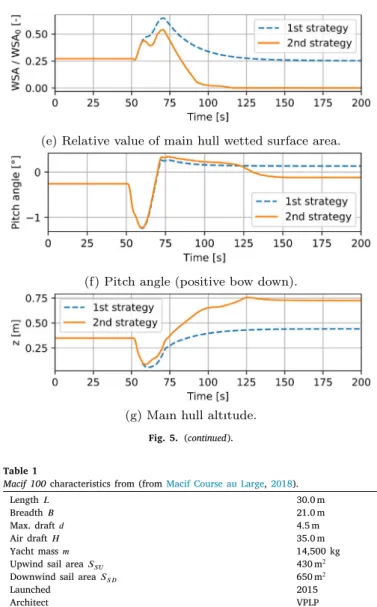
Fig. 5. Comparison of the two trimming strategies (Design 1).
to zero and �� adjusted by finding a compromise between the system’s
stability and settling time. Second, ��is increased to reduce oscillations
while avoiding excessive overshoots and instability.
4. Offshore trimaran simulations
This section presents three application cases of dynamic simulations: a maneuver, a case with unsteady wind on flat water and one in waves.
Fig. 5. (continued). Table 1
Macif 100 characteristics from (fromMacif Course au Large,2018).
Length � 30.0 m
Breadth � 21.0 m
Max. draft � 4.5 m
Air draft � 35.0 m
Yacht mass � 14,500 kg
Upwind sail area ��� 430 m2
Downwind sail area ��� 650 m2
Launched 2015
Architect VPLP
Shipyard CDK technologies
Table 2
First appendage configuration characteristics.
Foil Board Main rudder Float rudder
Max. depth (m) 1.9 3.6 1.8 1.6
Total span (m) 3.2 4.2 3.0 2.7
Mean chord (m) 0.9 1.1 0.5 0.4
4.1. Considered yacht
This section presents three simulation examples which underline specificities and interests of dynamic studies compared to steady ones. The simulated yacht is Macif 100, an offshore trimaran of the Ultim class. Skippered by François Gabart, she has been the holder of the single-handed sailing around-the-world record since 2017 (in 42 days
16 h 40 min 35 s). Her main particulars are given inTables 1and2. The
first two simulations consider the appendage package that was used for
the circumnavigation (Fig. 3a): two small L-foils, one centerboard and
three T-rudders (one on each hull), in the last simulation a second set
of appendages is used (Fig. 3b), with a larger foil and an elevator on
the centerboard. The windward foil is raised to the upper position in all examples.
Fig. 6. Distribution of vertical forces (in Earth fixed frame) as a percentage of yacht displacement (Design 1).
4.2. Simple maneuver
As known by VPP engineers, a given configuration (the parameters of the VPP: appendage tunings, ballast, sail trim, etc.) may lead to different equilibrium states (and thus different boat speeds), especially when the yacht has the ability to sail in different modes (Archimedean, fully flying, hybrid). The aim of this first simulation is to illustrate this specificity by comparing two sail trimming strategies, while adapting to new sailing conditions, and showing that even though the final configuration is the same in both cases, the final state largely differs, with a substantial speed delta.
Flat water conditions are considered. The yacht initially sails
up-wind in 19 knots of up-wind at 50◦ True Wind Angle on port tack. The
simulation is carried out in six degrees of freedom, with no active control system other than an autopilot for the rudder angle. At � = 50 s, the target heading is increased by sixty degrees so that the yacht bears
away (seeFig. 4). No change of sail is allowed.
As explained in Section3.4, the sail polars give the sail forces at the
considered steady Apparent Wind Angle (AWA) for an optimal trim. In dynamic conditions, such an approach is an idealization as it means that the sails are trimmed for maximum driving force at the same rate as the Apparent Wind Angle varies. However, the maximum driving force may not be the tuning that allows the maximal speed.
Fig. 7. True Wind Direction evolution.
Fig. 8. Time series of hulls and foil vertical forces (in Earth fixed frame) as percentage of yacht displacement (Design 1).
VPP studies carried out to optimize initial and final states configura-tions (board extension, rudder rake, Flat and Twist, etc.) show that the sails must be de-powered (twisted) after the bearing away maneuver. The sail twist enables to lower the center of effort, which decreases the heeling moment at the cost of an increased drag coefficient. The compared strategies focus on the timing of this specific action. In the first one, twist is operated progressively, but directly after the rudder action, while in the second one, the sails are twisted only after the main hull is lifted out of the water.
Fig. 9. Dynamic simulation results compared to steady VPP optimization on the same True Wind Angle value (orange) and range (green) (Design 1). (For interpretation of the references to color in this figure legend, the reader is referred to the web version of this article.)
With the second strategy the yacht maintains a strong heeling moment which makes her heel and decreases the wetted area of the main hull. The yacht can then accelerate, increasing thus the lift force of the foil in a virtuous circle that sees the hulls dynamic buoyancy and drag replaced by the foil action. Finally, the sails need to be twisted to enable the heeling moment to be balanced (as the boat accelerates, the aerodynamic heeling moment keeps on increasing otherwise). Acting too soon, as in the first strategy, prevents the yacht, under-powered,
from lifting the main hull (Figs. 5c, and5g), with an implicated lack of
speed of more than 4.5 knots (Fig. 5a).
Pushed by the inertial forces after the start of the turn, the yacht keeps briefly a non negligible speed component in the direction of her initial motion, that is to windward. This explains the negative leeway
peak shown inFig. 5b.
The ratio of the main hull wetted surface area to its nominal value
is shown inFig. 5e. Its evolution is close to the heel angle behavior and,
while it saturates at about 25% when using the first strategy, it indeed tends to zero in the second case, which corresponds to flying the main hull.
The pitch angle evolution is visible inFig. 5f. Its evolution is driven
by three main phenomena. First, the appendage tuning is changed during the maneuver, altering the pitching moment generated initially. The tuning history being similar in both strategies, this does not cause the difference between their final state. Second, after the maneuver, speeds are higher in both strategies, and as the speed increases, the aerodynamic bow down moment increases, leading to a greater pitch
angle. Finally, a last factor is at stake in the second strategy: the main hull leaves the water and its pitching moment component vanishes. That is why the second strategy shows a lower pitch angle than the first one.
While the timing of the sail twist varies between both strategies, other parameters are altered when bearing away but with identical timing in both cases. It is for instance necessary to partially lift up the centerboard and to change the rake angle of foils and rudders. This modifies the balance of the boat and explains the perturbations seen on the time series.
Fig. 6shows the time evolution of the distribution of vertical forces (aligned with acceleration of gravity) as a percentage of the yacht displacement. On both strategies, the load transfer from the float to the foil as the speed increases is visible, allowing to accelerate even more as the foil has a substantially better lift to drag ratio at such speeds. As previously shown, in the second strategy, the main hull is lifted out of the water by the sails heeling moment and the displacement is transferred to the foil and to a lesser extent to the float. Finally, the foil carries 50% of the yacht in the first strategy while in the second strategy this percentage reaches 70%.
This simulation highlights an interesting aspect verified in full-scale: one must build up speed before setting on the final configuration and track. This is very important as – especially for foiling yachts which can evolve in very different modes – one given configuration does not lead to a unique equilibrium. Dynamic simulation allows to work on
Table 3
Wind sinusoidal components.
i Period [s] Intensity factor
1 41 0.04
2 17 0.03
3 7 0.02
4 6.5 0.005
5 5 0.01
the strategy necessary to reach the VPP optimized steady speed and to optimize those transient phases.
4.3. Behavior in unsteady wind conditions
This second simulation case aims at showing the interest of dy-namic studies to predict potentially critical situations when evolving in unsteady conditions. The consequences on the yacht behavior of an irregular wind are studied. For this example, unsteadiness is modeled by adding sinusoidal components to the mean True Wind Direction
TWD0while the True Wind Speed is kept constant at 18 knots:
TWD (�) = TWD0 [ 1 +∑ � ��sin ( 2� ��� )] (16)
The periods ��and the intensity factors ��of the five sinusoidal
com-ponents are chosen arbitrarily. They are given inTable 3. Periods are
chosen so that they are not multiples of each other, in order to increase the time necessary to observe a periodic behavior. Time evolution of
the True Wind Direction is visible inFig. 7over the time range of the
simulation, those variations impact both the Apparent Wind Speed and the Apparent Wind Angle.
Flat water conditions are considered. At � = 0, the simulation is launched from a VPP optimized equilibrium corresponding to TWA
110◦/ TWS 18 kn, so that the unsteady wind acts as a perturbation to
this situation. It is interesting to notice that, in such a configuration the boat speed is about 30 knots, and therefore a major component of the apparent wind. The fluctuations of the apparent wind are thus much smaller than the true wind variations. During the 400 s simulation
the standard deviation of the True Wind Direction is 4.3◦ and the
amplitude between extrema is 19.5◦, while the corresponding values
for the Apparent Wind Angle are respectively 1.4◦ and 6.1◦. Some of
the simulation outputs are shown inFigs. 8and9. The yacht is free
to move in 6 degrees of freedom, while an autopilot with a constant
heading target (��= 0◦) controls the rudders.
As can be seen fromFig. 8, the yacht evolves in hybrid mode, with
in average 50% of the yacht displacement sustained by the foil. One can notice three peaks where the heel angle almost reaches
12◦(at t equals 200, 280 and 320 s, seeFig. 9c). Consistently,Fig. 7
shows that they correspond to situations where the wind heads (TWD maxima as the yacht heads North on port tack). However, such values of the True Wind Angle are reached several times without resulting in such heel angle peaks. This demonstrates how the wind sequence has a strong impact on the yacht instantaneous behavior and proves how necessary time-domain simulations are for the complete understanding of the yacht behavior.
Similarly,Fig. 9shows in green the limits reached in a steady VPP
when the yacht configuration is kept constant and the True Wind Angle
ranges from 100◦ up to 120◦, the minimal and maximal values of
Fig. 7. The heel variations are highly correlated to the wind direction signal, but very high peaks occur incidentally. This shows, as could be expected, that steady state analysis can miss critical situations. On the contrary, the simulated boat speed is well contained within the VPP limits, as the wind oscillates too quickly for the speed to settle to the steady equilibrium values seen in VPP. The average speed during the simulated sequence is 29.3 knots, which is slightly below the speed reached in steady wind (29.5 knots).
Fig. 11. Normalized cross-correlation function between True Wind Direction and boat speed (a) and Heel angle (b) (the first peak is highlighted in the enlargement).
Unlike the other outputs, the boat speed presents a low frequency component strongly dominating the high frequency ones. This low-pass filtering can be explained by the loads’ dependency to the boat speed that tends to damp the response as well as, unlike heel or heave, the absence of a strong hydrodynamic stiffness. This can be verified by comparing the power spectral densities of the output signals with the
input one (Fig. 10), which consistently shows that the first component
of the speed PSD is largely dominant over the other components. On the contrary, the signals of angular position show a spectrum that is relatively close to the input one, with some additional very small harmonics. The fourth component being rather weak and close to the third one, it is hardly distinguishable in the shown spectra.
Another difference between the yacht attitudes and her horizontal velocity components is the delay with which they respond to the wind perturbation. This can be shown by computing the normalized
cross-correlation function between input and output signals (seeFig. 11). The
first peak height gives the strength of the correlation while the abscissa indicates the phase shift. As expected the heel angle is highly correlated to the True Wind Direction (maximum correlation coefficient of 0.90) with a very short 0.85 s lag. On the contrary, the boat speed, which is also well correlated (maximum correlation coefficient of 0.71), presents a much higher delay of 7.22 s.
This simulation case has shown that a VPP is unable to predict the critical phases that can occur in unsteady conditions and that may be detrimental to the yacht safety and performance. DVPPs allow to study
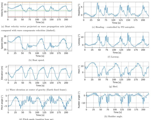
Fig. 12. Downwind sailing in waves results (Design 2). Table 4
Wave components properties.
i Period [s] Amplitude [m] Wavelength [m] Phase velocity [m/s]
1 10.46 1.69 171.1 16.34
2 6.92 0.49 74.8 10.80
3 4.15 0.18 26.9 6.48
these critical situations. Furthermore, they enable to study and improve the ship tuning parameters to optimize the speed in unsteady conditions and smooth even more the output signal. Besides, in such situations, the tuning of the autopilot coefficients may have significant impact on the response. DVPPs thus allow to study the effects of given coefficients and may be used within the tuning loop to optimize the behavior of on-board control systems.
4.4. Downwind sailing in waves
Finally, this third simulation case aims at modeling a sequence in the Southern Oceans (Indian or Pacific) which are generally almost totally sailed downwind in westerly winds. Southern ocean proper-ties corresponding to the period December–January have been chosen
based onYoung(1999). The sea state is constructed by superposition
of three wave components (Table 4) representing respectively the low,
medium and high frequency parts of a fully-developed spectrum of about 4.5 m significant wave height and 12.0 s peak period. All three components propagate in the same direction as the wind.
The pilot target is set at 140◦ of the wind direction. Results are
shown inFigs. 12and13.
Fig. 13. Hulls and foil vertical forces (in Earth fixed frame) as percentage of yacht displacement (Design 2).
While the phase velocities of the three wave components are
respec-tively 16.3, 10.8 and 6.5 m∕s (Fig. 12a), the yacht speed projected along
the wave propagation axis ranges between 9.7 and 15.0 m∕s. When caught up by the largest wave component, the yacht almost reaches its velocity. On the contrary, the smaller components are mostly overtaken by the yacht.
Fig. 12cshows the free surface elevation at the horizontal coordi-nates of the yacht center of gravity. The correspondence with the boat
speed evolution (Fig. 12b) is clearly visible. When the crests of the
largest wave component arrives at the ship (Fig. 14a), she is pushed
forward and surfs (between � = 25 s and 40 s for instance, seeFig. 14b).
The yacht mean speed is 30 knots but it undergoes very large variations, ranging from 25 up to 35 knots during the surfing phases.
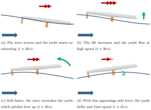
Fig. 14. Schematic sequence of the downwind simulation in waves (Blue arrows: wave propagation, red arrows: yacht speed, green arrows: yacht attitude evolution). (For interpretation of the references to color in this figure legend, the reader is referred to the web version of this article.)
As the yacht surfs in front of the coming wave, the orbital velocities further increase the appendage lift (by increasing the angle of attack, consequence of the wave vertical velocity component), especially of the
foils, and the yacht may reach a flying mode (Fig. 13). She remains
however slightly slower than the wave and is progressively overtaken. As it happens the effect of orbital velocities on the rear appendages is inverted (the wave vertical velocity becomes negative) and their lift decreases, as well as the efficiency of their pitch stabilizing effect.
The pitch angle is reduced (Figs. 12dand 14c) and the bow gains
altitude over the free surface. Consequently, the immersed surface of the foil shaft decreases, leading to a drop in the side force, making
the yacht bear away and drift (see Figs. 12e, 12f, for instance at
� = 40 s, and Fig. 14d). Drifting, and not pushed anymore by the
wave, the yacht slows down and reenters the water (Fig. 14e). It may
reach negative heel angles (Fig. 12g) due to the coupled effect of
decreased aerodynamic heeling moment (less apparent wind speed) and buoyancy on the leeward float bow that may touch the wave. The yacht finally realigns with her heading target as the pilot acts on the rudder (Fig. 12h), and the sequence starts again when another large wave arrives.
InFig. 12c, one can notice the presence of higher harmonics when elevation is positive and smoother behavior otherwise. A possible expla-nation would be that the appendages that carry the boat when elevation is large are more sensitive to small changes in the free surface elevation due to the high frequency waves than the hulls for which free surface
variations are averaged along a larger length. This is however not
clearly visible from the vertical loads time series (Fig. 13). A second,
more convincing, possible explanation is that the platform stability is higher when in Archimedean or hybrid mode than in flying mode, so that the high frequency perturbations are better filtered out.
It is interesting to note that the proportional coefficient of the heading autopilot (1.5 here) has a critical impact on the yacht behavior: with a too stiff autopilot the rudder corrections are too abrupt and the yacht drifts largely, while with a too small coefficient the yacht slaloms slowly, making very wide turns with substantial impacts on the velocity made to mark. The wave spectrum being fully developed and having a tight resonance peak, the first wave component is largely predominant over the others. A quasi-periodic behavior with frequency corresponding to the encounter frequency of this component can thus be observed on the provided time series. A pilot that would be aware of the position of the waves would be able to anticipate the yacht motion while she is overtaken. An autopilot algorithm with learning abilities would be able to recognize such a repeating pattern and determine an action to prevent it. Dynamic simulation allows to develop, train and test such controllers.
5. Conclusion
This paper describes the development and models of a numerical tool for sailing yacht dynamic behavior analysis. Example simulations
12
are presented to demonstrate the DVPP abilities, especially to study dynamic situations in which the yacht attitudes heavily differ from the corresponding steady state ones. In particular, it is shown how for identical values of the wind angle it is possible to observe highly different boat speed and attitudes depending on the recent history of the yacht and her environment. Examples of dynamic simulation show how the simulator can resolve the dynamic response of the yacht in unsteady wind and in waves as well as the sensibility of the yacht behavior to the tuning strategies, and the necessity for the user to find a tuning path to the VPP optimized boat speed.
This second design configuration proves to be closer to a flying mode – which is consistent with the increased size of the lifting surfaces – with a foil that carries in average 60% of the yacht displacement
(30% for the hulls, seeFig. 13) while for the first configuration in the
unsteady wind simulation the distribution was respectively 50% and 40%(Fig. 8). The last 10% are mainly distributed between the T-rudders. The lifting board of design 2 has a small averaged contribution as, due to the large trim variations it regularly exerts a negative lift force. Its main interest resides here in a stabilizing effect.
Such a numerical tool therefore brings a relevant help to yacht designers and sailors in order to predict and identify critical situations where the dynamic stability and performance of the yacht can be affected. Furthermore, from such a non-linear model, it is possible to derive simpler models for specific use. One may for instance compute the load derivatives to perform stability analysis around given equi-librium points and derive the eigenvectors and natural modes of the
system (Heppel, 2015), which can then be compared to actual
time-domain simulation. Deriving linear models from the initial non-linear
one is also of great help for control systems tuning (Legursky,2013).
To further study the motion stability, deriving dedicated criteria and quantities based on dynamic simulations should help assess the quality of given appendages design.
Further work is however still needed, especially regarding ap-pendages and aerodynamic loads, to handle a wider range of dynamic situations, for instance to model imperfectly trimmed sails.
CRediT authorship contribution statement
Paul Kerdraon: Methodology, Software, Writing - original draft. Boris Horel: Supervision, Writing - review & editing. Patrick Bot:
Su-pervision, Writing - review & editing. Adrien Letourneur: SuSu-pervision, Writing review & editing. David Le Touzé: Supervision, Writing -review & editing.
Declaration of competing interest
The authors declare that they have no known competing finan-cial interests or personal relationships that could have appeared to influence the work reported in this paper.
Acknowledgments
This work was supported by VPLP Design, France and the ANRT (French National Association for Research and Technology).
References
Abkowitz, M.A., 1964. Lectures on Ship Hydrodynamics - Steering and Manoeuvra-bility. Report no. Hy-5, Hydrodynamics Department, Hydro- and Aerodynamics Laboratory, Lyngby, Denmark.
Augier, B., Hauville, F., Bot, P., Aubin, N., Durand, M., 2014. Numerical study of a flexible sail plan submitted to pitching: Hysteresis phenomenon and effect of rig adjustements. Ocean Eng. 90, 119–128.
Binns, J.R., Hochkirch, K., De Bord, F., Burns, I.A., 2008. The development and use of sailing simulation for IACC starting manoeuvre training. In: 3rd High Performance Yacht Design Conference. Auckland, New Zealand. pp. 158–167.
Claughton, A., 1999. Developments in the IMS VPP formulation. In: The 14th Chesapeake Sailing Yacht Symposium. Annapolis, MD, USA.
Cummins, W.E., 1962. The Impulse Response Function and Ship Motion. Report 1661, Navy Department, David Taylor Model Basin – Hydromechanics Laboratory, MD, USA.
Day, S., Letizia, L., Stuart, A., 2002. VPP vs PPP: challenges in the time-domain prediction of sailing yacht performance. In: High Performance Yacht Design Conference. Auckland, New-Zealand.
Delhommeau, G., 1987. Les Problèmes de Diffraction-Radiation et de Résistance de Vagues : Étude Théorique et Résolution Numérique par la Méthode des Singularités (Ph.D. thesis). Ecole Nationale Supérieure de Mécanique, Nantes, France.
Fossati, F., Muggiasca, S., 2011. Experimental investigation of sail aerodynamic behavior in dynamic conditions. J. Sailboat Technol. Society of Naval Architects and Marine Engineers.
Gerhardt, F.C., Flay, R., Richards, P., 2011. Unsteady aerodynamics of two interacting yacht sails in two-dimensional potential flow. J. Fluid Mech. 668, 551–581. Gerhardt, F.C., Le Pelley, D., Flay, R., Richards, P., 2009. Tacking in the wind tunnel. In:
The 19th Chesapeake Sailing Yacht Symposium. Annapolis, MD, USA. pp. 161–175. Harris, D.H., 2005. Time domain simulation of a yacht sailing upwind in waves. In: The 17th Chesapeake Sailing Yacht Symposium. Annapolis, MD, USA. pp. 13–32. Heppel, P., 2015. Flight dynamics of sailing foilers. In: 5th High Performance Yacht
Design Conference. Auckland, New Zealand. pp. 180–189.
Horel, B., 2016. Modélisation Physique du Comportement du Navire par mer de l’Arrière (Ph.D. thesis). Ecole Centrale de Nantes, France.
Horel, B., 2019. System-based modelling of a foiling catamaran. Ocean Eng. 171, 108–119.
Jackson, P., 2001. An improved upwind sail model for VPPs. In: The 15th Chesapeake Sailing Yacht Symposium. Annapolis, MD, USA. pp. 11–20.
Jacquin, E., Guillerm, P.-E., Derbanne, Q., Boudet, L., Alessandrini, B., 2005. Simulation d’essais d’extinction et de roulis forcé à l’aide d’un code de calcul Navier-Stokes à surface libre instationnaire. In: 10èmes Journées de L’Hydrodynamique. Nantes, France.
Katz, J., Plotkin, A., 2001. Low-Speed Aerodynamics. Cambridge University Press. Kerwin, J.E., 1978. A Velocity Prediction Program for Ocean Racing Yachts Revised
to June 1978. H. Irving Pratt Project Report 78–11, Massachusetts Institute of Technology, Cambridge, MA, USA.
Keuning, J.A., Vermeulen, K.J., De Ridder, E.J., 2005. A generic mathematical model for the maneuvering and tacking of a sailing yacht. In: The 17th Chesapeake Sailing Yacht Symposium. Annapolis, MD, USA. pp. 143–163.
Larsson, L., 1990. Scientific methods in yacht design. Annu. Rev. Fluid Mech. 22 (1), 349–385.
Legursky, K., 2013. Least squares estimation of sailing yacht dynamics from full-scale sailing data. In: The 21st Chesapeake Sailing Yacht Symposium. Annapolis, MD, USA.
Lindstrand Levin, R., Larsson, L., 2017. Sailing yacht performance prediction based on coupled CFD and rigid body dynamics in 6 degrees of freedom. Ocean Eng. 144, 362–373.
Macif Course au Large, 2018. Le trimaran Macif.https://www.macifcourseaularge.com/ trimaran-macif/bateau/. [Online; accessed 10-September-2018].
Masuyama, Y., Fukasawa, T., Sasagawa, H., 1995. Tacking simulation of sailing yachts – Numerical integration of equations of motion and application of neural network technique. In: The 12th Chesapeake Sailing Yacht Symposium. Annapolis, MD, USA. Masuyama, Y., Nakamura, I., Tatano, H., Takagi, K., 1993. Dynamic performance of sailing cruiser by full-scale sea tests. In: The 11th Chesapeake Sailing Yacht Symposium. Annapolis, MD, USA. pp. 161–179.
Oliver, J.C., Letcher, Jr., J.S., Salvesen, N., 1987. Performance predictions for Stars & Stripes. In: SNAME Trans., Vol. 95. New York, NY, USA. pp. 239–261. Richardt, T., Harries, S., Hochkirch, K., 2005. Maneuvering simulations for ships
and sailing yachts using FRIENDSHIP-Equilibrium as an open modular work-bench. In: International EuroConference on Computer Applications and Information Technology in the Maritime Industries, COMPIT. Hamburg, Germany. pp. 101–115. Roux, Y., Durand, M., Leroyer, A., Queutey, P., Visonneau, M., Raymond, J., Finot, J.-M., Hauville, F., Purwanto, A., 2008. Strongly coupled VPP and CFD RANSE code for sailing yacht performance prediction. In: 3rd High Performance Yacht Design Conference. Auckland, New Zealand. pp. 215–226.
Tuckerman, L.B., 1926. Inertia Factors of Ellipsoids for Use in Airship Design. TR 210, National Advisory Committee for Aeronautics, Washington, DC, USA.
Young, I.R., 1999. Seasonal variability of the global ocean wind and wave climate. Int. J. Climatol. 19 (9), 931–950.