Decomposition algorithms for global solution of deterministic and stochastic pooling problems in natural gas value chains

Decomposition Algorithms for Global Solution of

Deterministic and Stochastic Pooling Problems in Natural

Gas Value Chains

by

Emre Armagan

Submitted to the Department of Mechanical Engineering

in partial fulfillment of the requirements for the degree

oA

MASSACHUSETTS INSTITWE OF TECHN!OLOGY

Master of Science in Mechanical Engineering

[

at the

L

BTRARIES

MASSACHUSETTS INSTITUTE OF

TECHNOLOGY

L-January 2009

© Massachusetts Institute of Technology 2009. All rights reserved.

A uthor ...

Departm nt of Mchanical Engineering

January 28, 2009

Certified by ...

Certified by ....

Professor,

Paul I. Barton

Professor, Department of Chemical Engineering

Thesis Supervisor

Stephen C. Graves

Department of Mechanical Engineering and Management

S~

T

Supervisor

Accepted by...

David E. Hardt

Chairman, Department Committee on Graduate Students

Decomposition Algorithms for Global Solution of Deterministic and

Stochastic Pooling Problems in Natural Gas Value Chains

by

Emre Armagan

Submitted to the Department of Mechanical Engineering

on January 28, 2009, in partial fulfillment of the

requirements for the degree of

Master of Science in Mechanical Engineering

Abstract

In this thesis, a Benders decomposition algorithm is designed and implemented to solve

both deterministic and stochastic pooling problems to global optimality. Convergence of

the algorithm to a global optimum is proved and then it is implemented both in GAMS and

C++ to get the best performance. A series of example problems are solved, both with the

proposed Benders decomposition algorithm and commercially available global

optimiza-tion software to determine the validity and the performance of the proposed algorithm.

Moreover, a two stage stochastic pooling problem is formulated to model the optimal

ca-pacity expansion problem in pooling networks and the proposed algorithm is applied to

this problem to obtain global optimum. A number of example stochastic pooling problems

are solved, both with the proposed Benders decomposition algorithm and commercially

available global optimization software to determine the validity and the performance of the

proposed algorithm applied to stochastic problems.

Thesis Supervisor: Paul I. Barton

Title: Professor, Department of Chemical Engineering

Thesis Supervisor: Stephen C. Graves

Acknowledgments

First and foremost, I would like to thank my parents, Gulden and Kadri Armagan, for their

love and support. Without their help this degree would not have been possible.

I would like to thank my thesis supervisor Professor Paul I. Barton for his direction,

assistance, and guidance. His recommendations and suggestioris have been invaluable for

the project and for this thesis. I am grateful to Professor Stephen C. Graves for reading and

evaluating my thesis.

I also wish to thank Professor Asgeir Tomasgard and Lars Hellemo from Norwegian

University of Science and Technology (NTNU). Professor Tomasgard's assistance and

sug-gestions have been a tremendous help.

I am indebted to Ajay Selot who helped me whenever I need assistance and helped

me to learn necessary programming skills. In addition, I am also grateful to all of my

colleagues in the Process Systems Engineering Laboratory, especially Patricio Ramirez,

for their support and encouragement.

This research was supported by funding from StatoilHydro, SINTEF and NTNU. I

would like to thank them all for their financial support.

Contents

1 INTRODUCTION 17

1.1 POOLING PROBLEMS.. .. .... ... ... . ... .... . . 17

1.2 IMPORTANCE OF POOLING PROBLEMS IN THE NATURAL GAS VALUE CHAIN ... ... ... 19

1.3 BENDERS DECOMPOSITION FOR THE GLOBAL SOLUTION OF POOLING PROBLEMS . ... ... 21

2 PROBLEM DEFINITION 23 2.1 THE P-, Q- AND PQ-FORMULATIONS . ... . .... ... . .... 29

3 LITERATURE REVIEW 33 3.1 DETERMINISTIC POOLING PROBLEM . . . ... . .. . ... . . 33

3.2 INFRASTRUCTURE DEVELOPMENT AND THE STOCHASTIC POOLING PROB-LEM . . . ... . . 36

4 BD ALGORITHM FOR DETERMINISTIC POOLING PROBLEM 41 4.1 INTRODUCTION OF BENDERS DECOMPOSITION ALGORITHM . ... 41

4.2 PROOF OF CONVERGENCE ... . .. ... ... .. 46

4.3 IMPLEMENTATION ... ... 50

4.3.1 GAMS IMPLEMENTATION ... .. ... .... 50

4.3.3 RESULTS ... ... ... ... 58

5 APPLICATION TO THE STOCHASTIC POOLING PROBLEM 61 5.1 INFRASTRUCTURE DEVELOPMENT PROBLEMS IN NATURAL GAS VALUE CHAIN ... ... ... ... .. 61

5.2 INTRODUCTION TO STOCHASTIC PROGRAMMING ... . ... .... . 63

5.3 IMPORTANCE OF STOCHASTIC POOLING PROBLEMS IN NATURAL GAS INFRASTRUCTURE DEVELOPMENT ... ... . ... . 65

5.4 FORMULATION OF THE STOCHASTIC POOLING PROBLEM . . .... .. 67

5.5 IMPLEMENTATION OF THE BD ALGORITHM IN STOCHASTIC POOLING PROBLEMS... ... ... . ... 73

5.6 RESULTS . ... ... ... . 78

6 CONCLUSION 83 A EXAMPLE POOLING PROBLEMS 87 A.1 ADHYA'S POOLING PROBLEM . . ... . ... . . . .... 87

A.2 FOULDS' POOLING PROBLEM . . ... . .. . . . ... 89

A.3 EXAMPLE 1 ... . 91

A.4 EXAMPLE2 ... ... ... 91

A.5 EXAMPLE 3 ... ... ... .... 91

A.6 EXAMPLE 4 ... . 92

B GAS NETWORK EXAMPLE 121 C THE STOCHASTIC POOLING PROBLEM 135 C.1 STOCHASTIC EXAMPLE I . ... . .... . ... . .... 136

C.2 STOCHASTIC EXAMPLE 2 . ... ... ... . 138

C.3 STOCHASTIC EXAMPLE 3 ... ... . ... 140

C.4 STOCHASTIC EXAMPLE 4 .. ... . 142

List of Figures

2-1 Graphical representation of a general pooling problem .... ... . 24

2-2 Haverly's pooling problem ... ... ... . 27

2-3 The q-formulation of the Haverly's pooling problem ... 29

2-4 The pq-formulation of the Haverly's pooling problem ... 30

4-1 Flowchart of the proposed BD algorithm ... ... .... . 48

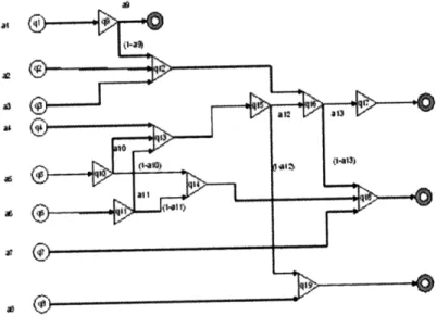
4-2 The gas network example ... . 55

5-1 Basic illustration of decomposition algorithms in stochastic programming . 66 B-1 Representation of a mixer (a) and splitter (b) . ... . .... ... 122

List of Tables

2.1 Parameters of the pooling problem and corresponding definitions . ... . 25

2.2 Solution times for the p-,q- and pq- formulations in example problems (in seconds). ... ... ... ... 31

4.1 Optimal objective values in GAMS .... ... ... 52

4.2 Solution times in GAMS (in seconds) ... ... 53

4.3 Solution times for the gas network problem (in seconds) . ... 55

4.4 Solution times in C++ with and without Range Reduction (in seconds) . . . 58

4.5 Solution times in C++ (in seconds) ... ... . . 58

5.1 Parameters and corresponding definitions for the first stage problem . . .. 70

5.2 Parameters and corresponding definitions for the second stage problem ... 71

5.3 Solution times of stochastic pooling problems with one quality variable (in minutes) ... ... ... 80

5.4 Solution times of stochastic pooling problems with two quality variables (in minutes) ... ... ... ... 80

5.5 Solution times of stochastic pooling problems with three quality variables (in minutes) ... ... 80

A. 1 Quality parameters in source nodes for Adhya's problem ... ... . 88

A.2 Cost parameters in source nodes for Adhya's problem . ... 88

A.4 Flow requirements in demand nodes for Adhya's problem . A.5 A.6 A.7 A.8 A.9 A.10 A.11 A.12 A.13 A.14 A.l15 A.16 A.17 A.18 A.19 A.20 A.21 A.22 A.23 A.24 A.25 A.26 A.27 A.28 A.29 A.30

Prices in demand nodes for Adhya's problem . ... 89

Quality parameters in source nodes for Foulds' problem . ... 89

Cost parameters in source nodes for Foulds' problem ... ... 90

Quality requirements in demand nodes for Foulds' problem ... 90

Flow requirements in demand nodes for Foulds' problem . ... 90

Prices in demand nodes for Foulds' problem . ... 91

Quality parameters in source nodes for Example 1 ... .... 92

Cost parameters in source nodes for Example 1 ... ... 93

Quality requirements in demand nodes for Example 1 ... ... 93

Flow requirements in demand nodes for Example 1 . ... .. 94

Prices in demand nodes for Example 1 ... . .. . . . 94

Quality parameters in source nodes for Example 2 ... ... . 95

Cost parameters in source nodes for Example 2 . ... 96

Quality requirements in demand nodes for Example 2 . ... 96

Flow requirements in demand nodes for Example 2 . ... 97

Prices in demand nodes for Example 2 ... ... 97

Quality parameters in source nodes for Example 3 . ... 98

Cost parameters in source nodes for Example 3 . ... . 98

Quality requirements in demand nodes for Example 3 . ... 99

Flow requirements in demand nodes for Example 3 ... ... 99

Prices in demand nodes for Example 3 ... . 99

Quality parameters in source nodes for Example 4 . ... 100

Cost parameters in source nodes for Example 4 ... ... 100

Quality requirements in demand nodes for Example 4 . ... ..101

Flow requirements in demand nodes for Example 4 . ... 101

B. 1 Quality parameters in source nodes for the gas network example ... 123 B.2 Cost parameters in source nodes for the gas network example ... 123 B.3 Quality requirements in demand nodes for the gas network example . . . . 123

B.4 Flow requirements in demand nodes for the gas network example ... . 123 B.5 Prices in demand nodes for the gas network example . ... 124

C. 1 Source quality parameters in scenarios and the respective probability values 136 C.2 First stage investment costs of pools for Stochastic Example I ... . 136 C.3 First stage investment costs of pipelines (sources to pools) for Stochastic

Example 1 ... 137 C.4 First stage investment costs of pipelines (pools to demands) for Stochastic

Example 1 ... . ... ... .137 C.5 Second stage cost parameters in source nodes for Stochastic Example 1 . .137 C.6 Second stage quality requirements in demand nodes for Stochastic

Exam-plel... 137 C.7 Second stage flow requirements in demand nodes for Stochastic Example 1 137 C.8 Second stage prices in demand nodes for Stochastic Example 1 ... 137 C.9 First stage investment costs of pools for Stochastic Example 2 ... 138 C.10 First stage investment costs of pipelines (sources to pools) for Stochastic

Example2 ... ... . ... 138 C. 11 First stage investment costs of pipelines (pools to demands) for Stochastic

Example 2... ... 138 C. 12 Second stage cost parameters in source nodes for Stochastic Example 2 . .139 C.13 Second stage quality requirements in demand nodes for Stochastic

Exam-ple 2 ... ... 139 C. 14 Second stage flow requirements in demand nodes for Stochastic Example 2 139 C. 15 Second stage prices in demand nodes for Stochastic Example 2 ... 139 C.16 First stage investment costs of pools for Stochastic Example 3 ... 140

C. 17 First stage investment costs of pipelines (sources to pools) for Stochastic Example 3 ... ... ... 140 C. 18 First stage investment costs of pipelines (pools to demands) for Stochastic

Example 3 ... ... 140 C. 19 Second stage cost parameters in source nodes for Stochastic Example 3 . . 141 C.20 Second stage quality requirements in demand nodes for Stochastic

Exam-ple3... ... 141 C.21 Second stage flow requirements in demand nodes for Stochastic Example 3 141 C.22 Second stage prices in demand nodes for Stochastic Example 3 ... 141 C.23 First stage investment costs of pools for Stochastic Example 4 .... . .. 142

C.24 First stage investment costs of pipelines (sources to pools) for Stochastic Example 4... ... 143 C.25 First stage investment costs of pipelines (pools to demands) for Stochastic

Example 4... ... ... 143 C.26 Second stage cost parameters in source nodes for Stochastic Example 4 . . 144 C.27 Second stage quality requirements in demand nodes for Stochastic

Exam-ple4 ... ... ... 144 C.28 Second stage flow requirements in demand nodes for Stochastic Example 4 144 C.29 Second stage prices in demand nodes for Stochastic Example 4 . .... .. 145

Chapter 1

Introduction

1.1 Pooling Problems

The pooling problem is a planning problem that arises in blending materials to produce products; an example might be the blending of petroleum or natural gas. Pooling occurs whenever streams are mixed together, often in a storage tank, and the resulting mixture is distributed to several locations. Pooling and blending of raw materials and stored products is an important step in the synthesis of end products having different quality specifications. Products possessing different attribute qualities are mixed in a series of pools in such a way that the attribute qualities of the blended products of the end pools must satisfy given re-quirements. Pooling also occurs in distillation and other separation processes. The mathe-matics of the pooling problem applies to such processes and their applications. In a pooling problem, each material has a set of attributes with associated qualities, such as percentage of sulfur or carbon dioxide percentage. Pool qualities are defined by a flow-weighted aver-age of the source qualities and product qualities are similarly defined by a flow-weighted average of the pool qualities. Product qualities are constrained to lie in specified ranges. The pooling problem is to maximize the total profit, subject to flow and quality constraints. The pooling problem is a bilinear optimization problem because the output stream

qual-ities, which are unknown, depend on the flowrates, which is also unknown, and on the quality of the input streams. Because of the bilinear terms, the process of pooling intro-duces nonlinearities and nonconvexities into optimization models leading to the possibility of several locally optimal solutions some of which may be suboptimal. Naturally, it takes more effort to solve a problem to guaranteed global optimality than it takes to find a locally optimal solution and one must often weigh the benefits against the costs. However, it is ap-parent that global optimization of the pooling and blending process could lead to substantial

savings in cost, resulting in higher profits as in the case of the petroleum industry.

Numerical algorithms for solving pooling problems have included sensitivity and feasi-bility analysis and local optimization techniques. However, because of the benefits of solv-ing poolsolv-ing problems to guaranteed global optimality as explained above, more recently deterministic global optimization algorithms (which use Branch-and-Bound, Benders De-composition (BD) or Generalized Benders DeDe-composition (GBD), etc.) have also been proposed. However, the application of global optimization algorithms to the pooling prob-lem continues to be a challenge because of the slow convergence speed of the proposed algorithms. Since the nonconvexities and nonlinearities of a pooling problem come from the bilinear terms, a BD or GBD based algorithm looks as a promising approach in order to find the global optimal solution of the problem. Moreover, decomposition algorithms are often regarded as better candidates to solve stochastic infrastructure development prob-lems in the natural gas value chains, which is the ultimate objective of this project. How-ever, as explained in the later sections of this thesis, until now in the literature, in order to solve pooling problems to global optimality with GBD algorithms (in the literature, a BD algorithm has not yet been proposed for the solution of pooling problems), only one of the variables appearing in the bilinear terms was taken as the complicating variable (de-tailed information about BD and GBD algorithms is provided in Chapter 4) and with this approach even for relatively simple pooling problems, the proposed GBD algorithms con-verge to suboptimal solutions, even non-KKT points, and therefore does not guarantee a

global optimum.

1.2

Importance of Pooling Problems in the Natural Gas

Value Chain

Natural gas is a vital component of the world's supply of energy and its importance has been increasing as a fossil fuel in recent years because of different factors. First of all, unlike other fossil fuels, natural gas is a relatively clean fuel since it emits low levels of potentially harmful byproducts such as sulphur particulates, carbon dioxide and nitrogen oxides, as it bums. In addition, from the geographical perspective, natural gas is more uniformly distributed than oil. Moreover, since it is relatively easy, cheap and clean to convert it into hydrogen, natural gas is considered to be one of the most important elements in the transition to a hydrogen economy.

Raw natural gas typically consists primarily of methane (CH4), the shortest and lightest

hydrocarbon molecule. It also contains varying amounts of heavier gaseous hydrocarbons

(ethane (C2H6), propane (C3H8), butane (C4H1 0), etc.), acid gases (carbon dioxide (CO2), hydrogen sulfide (H2S), etc.), nitrogen (N2), helium (He) and water vapor. All of those

gases except methane are called the impurities and the raw natural gas must be purified to meet the quality standards specified by the contractual agreements between production companies and major pipeline transmission and distribution companies. Those quality stan-dards vary from pipeline to pipeline and are usually a function of a pipeline systems design and the markets that it serves. In general, the standards specify that the natural gas be within a specific range of heating value (For example, in the United States, it should be about 1,035 + 5% Btu per cubic foot of gas at 1 atmosphere and 60 'F); be delivered at or above a specified hydrocarbon dew point temperature; be free of particulate solids and liquid water to prevent erosion, corrosion or other damage to the pipeline; be dehydrated of water vapor sufficiently to prevent the formation of methane hydrates within the gas

processing plant or pipeline; contain no more than trace amounts of components such as hydrogen sulfide, carbon dioxide, nitrogen, and water vapor [10].

If natural gas is transported in the form of liquefied natural gas (LNG), during LNG production, the liquefaction process involves condensation of natural gas into liquid form by cooling it to approximately -163 'C (-260 'F). The natural gas fed into the LNG plant has to be treated to remove water, hydrogen sulfide, carbon dioxide and other components that will freeze under the low temperatures needed for storage or be destructive to the liquefaction facility.

Moreover, with the advent of sustained higher natural gas prices and declining reserves, and as technology and geological knowledge advances, so-called "unconventional" natural gas sources are coming to market. Although, there are many different sources of "uncon-ventional" natural gas today, one common characteristic of all is the higher concentration of acid gases compared to "conventional" natural gas sources. Therefore, as technology ad-vances, large amounts of off-spec natural gas becomes available that does not meet pipeline quality without some sort of adjustment. This off-spec gas has to be processed to meet the requirements before being pumped into pipelines.

Hence, to transport natural gas from fields to consumers by any means or to make "un-conventional" natural gas available to consumers, it is required to reduce the concentration of undesired molecules. Two methods exist to achieve this goal: purification and blending. The process of purification of natural gas to pipeline gas quality levels is quite complex, highly capital-intensive and usually involves four main processes to remove the various impurities: oil and condensate removal, water removal, separation of natural gas liquids, sulfur and carbon dioxide removal. These processes become more complex and therefore more expensive, as the concentration of the impurities increases in the natural gas being purified and increases the cost of the natural gas for consumers while reducing the prof-its of the production companies. Detailed information about purification processes can be found in Guo and Ghambalor (2005) [17].

Blending of natural gas from different fields or wells with different different concentra-tions of hydrocarbons, carbon dioxide, hydrogen sulfide and nitrogen is a cheaper method. However, it does not always guarantee achievement of the desired concentration levels. But, blending can be utilized to reduce the concentrations of undesired molecules before purification processes in order to reduce the cost of the purification. The opportunity for blending different sources of natural gas comes into the picture especially when the natural gas production infrastructure is being developed. When new wells or fields are being de-veloped, it is possible to construct the pipeline system such that the gas from different wells are mixed together to satisfy the requirements for different qualities. However to develop the pipeline system optimally, a stochastic version of the pooling problem where the qual-ity parameters in the wells are not known exactly has to be solved. Although advancing technology provides the necessary tools to predict the gas content of natural gas in different fields during the exploration stage, the impurities in the natural gas are still uncertain before drilling the well. Thus, stochastic programming principles have to be used to achieve an optimum solution to the infrastructure development problem. As mentioned, in this study, one of the important reasons to develop a BD algorithm to solve pooling problems is the adaptability of decomposition algorithms to stochastic programming. More information about the stochastic pooling problem is given in Chapter 5 of this thesis.

1.3

Benders Decomposition for the Global Solution of

Pool-ing Problems

As explained in Section 4.1, BD and GBD algorithms are proposed to solve multi-variable nonlinear programs and take at least one of the variables appearing in bilinear terms as fixed to solve the problem. In the literature, in order to solve pooling problems to global optimality with GBD, only one of the variables appearing in the bilinear terms was taken as the complicating variable. With this approach, even for relatively simple pooling problems,

the GBD algorithm tends to generate suboptimal points and does not guarantee to attain a global optimum. For instance, Floudas & Aggarwal (1990) [11] use the GBD algorithm to solve pooling problems by fixing the pool quality variables as the complicating variables and decompose the original pooling problem into a primal problem and a relaxed master problem. But, their strategy is only successful for Haverly's pooling problem (which is a very simple problem) and in general, it offers no guarantee for global optimality. This GBD algorithm may converge to a local minimum, a local maximum, or even a non-KKT point. In this study, both of the variables appearing in bilinear terms are treated as the com-plicating variables and by doing so the problem can be formulated such that the Benders Decomposition algorithm can be used instead of Generalized Benders Decomposition and hence satisfaction of the Property P becomes unnecessary and, unlike Floudas & Aggarwal (1990) [11], convergence is guaranteed and can be proven directly from Benders (1962)

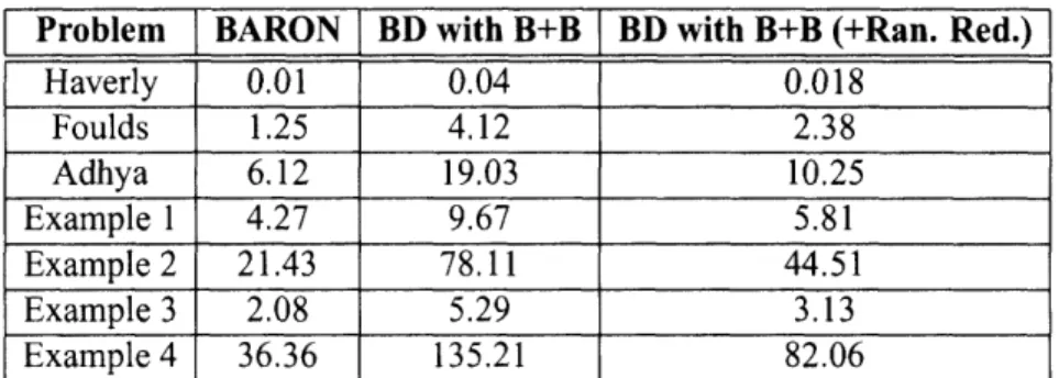
[5]. Fixing both variables in the bilinear terms provides a linear program in the first stage of the algorithm and smaller (and hence easier to solve) bilinear second stage problems. For comparison of the proposed algorithm with a well known and respected global solver, The Branch And Reduce Optimization Navigator (BARON) is selected [42]. BARON is a com-putational software developed by Nikolaos Sahinidis and Mohit Tawarmalani for solving nonconvex optimization problems to global optimality. Purely continuous, purely integer, and mixed-integer nonlinear problems can be solved with this software. BARON com-bines constraint propagation, interval analysis, range (domain) reduction and duality with enhanced Branch-and-Bound (B+B) concepts to solve optimization problems globally. In general, BARON is a nonconvex optimization solver using range reduction methods in-tegrated into the B+B algorithm with advanced relaxation techniques [39]. In this study, in order to check global optimality and validity of the approach, various example pooling problems are solved with both the proposed BD algorithm and BARON. In addition, the solution times of the BD algorithm and BARON are compared to study the overall perfor-mance of BD for pooling problems.

Chapter 2

Problem Definition

In general, the pooling problem can be stated in a general way as follows: given several streams with different qualities, what quantities of each must be mixed in intermediate pools in such a way that the quality and quantity requirements of all demands are satisfied. A pooling network consists of several source nodes, pools and end-product nodes. Each source node has a unique quantity of available supply and quality components. Sources are linked to pools and each pool represents a blend from various source nodes and the quality component of a pool is a function of the levels of in-flows from sources and their qualities. Pools are linked to product nodes and each pool's total in-flow is equal to its total out-flow (mass balance). The quality component of a product node is also a function of the levels of in-flows from sources and pools and their qualities. Product nodes are subject to specific demand and quality requirements. In practice, because of the presence of a large number of supply nodes, pools, qualities and end-products, pooling problems are more complicated than expected. Usually, each stream into a pool can have more than one quality compo-nent. The pooling problem then becomes a problem with multiple component qualities and every end product has to be in the range of expected quality specifications for each of the quality components. The existence of multiple pools, products and qualities creates hun-dreds of bilinear terms even for a relatively small problem and therefore a large number of

suboptimal local minima can also exist, hence the need for a global optimization approach increases.

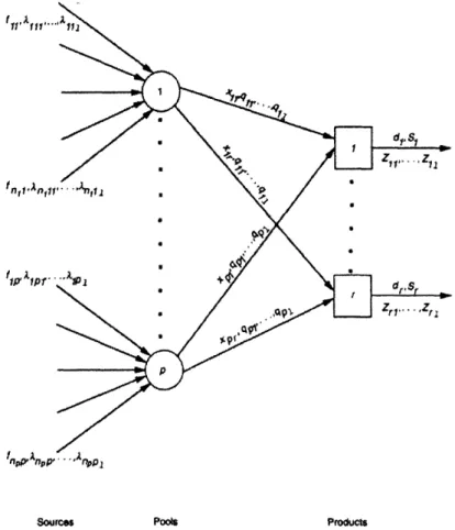
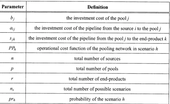
Figure 2-1 shows a general pooling problem with n sources, p pools, r end-products and / quality parameters. In this representation, i is the index for sources, j is the index for pools, k is the index for products and w is the index for qualities. In addition, fjj is the variable for the total flow from the ith source into poolj; qjw is the variable for the wth quality component of pool j and xjk is the variable for the total flow from the jth pool to product k. Also parameters in this representation are listed in Table 2.1.

Ztl .. ' Zl1

fi .t

ZrI.. -.. Zrl

f Ap~.'qp

Sources Pool Products

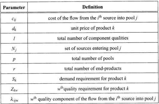
Parameter Definition

C . cost of the flow from the ith source into poolj

dk unit price of product k

1 total number of component qualities Nj set of sources entering poolj

p total number of pools

r total number of end-products

Sk demand requirement for product k

Zkw wthquality requirement for product k

kjjw Wt h quality component of the flow from the ith source into poolj Table 2.1 : Parameters of the pooling problem and corresponding definitions

Then, a mathematical representation of the general pooling problem that is represented in Figure 2-1 becomes: (2.1) s.t.

_I

j

j

fli < fI < fi- , i= 1,...,nj; j = 1,...,p

<fqj,

k<

<

xk,

j=

1,...,p; k= 1,...,r

In this formulation, the objective function represents the difference between the cost of the flow from the source nodes and the returns from selling the end-products. (2.2) represents the mass balances for each pool. (2.3) expresses the mass balance for each quality component. (2.4) ensures that the flows to each end-product node do not exceed the demands. (2.5) enforces that the quality requirements are satisfied at each end-product node. More information about the formulation can be found in Audet et. al. (2004) [3].

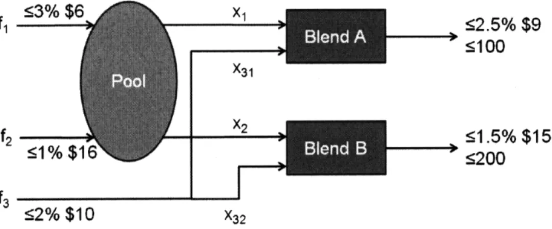
In addition, in the literature there are some widely known and solved pooling problem formulations which are just special cases of this general representation. These problems are solved in numerous papers about the pooling problem and hence their global optimal solutions are known and there are different global optimization algorithms, which have already been proven to converge, available for them, which can be used for comparison with the BD algorithm. Thus, these problems can be used as examples to check the validity and performance of the proposed BD algorithm. The pooling problem was first investigated by Haverly (1978-1979) [19, 20]. Therefore, Haverly's pooling problem is one of these widely known pooling problems and it consists of only 3 source nodes, 1 pool and 2 demand nodes as shown in Figure 2-2. Figure clearly represents that three feed streams are available (fi, f2 and f3), with the costs of $6, $16 and $10 (per unit) respectively. There are also two output streams with the prices of $9 and $15 (per unit) respectively.

In Haverly's pooling problem, there is a single pool which receives supplies from two different sources which have different sulfur qualities. A third supply is not connected to

X1 X31 X2

I

5100

51.5% $15

:200

Figure 2-2: Haverly's pooling problem

the pool but is directly feeding the two end-product nodes. The quality parameters for the streams going into the pool are 3% for the first source node, 1% for the second and 2% for the third node. The blending of flows from the pool and from the third supply node produces products 1 and 2, which are subjected to sulfur quality requirements of 2.5% and 1.5% respectively. The maximum demands for products 1 and 2 are 100 and 200 respectively. Then the mathematical formulation of Haverly's pooling problem is:

min

6ft

+ 16f

I

53% $6

52% $10

(2.6)

(2.8)

(2.10)

P

N ln

qx12 +2X22 - 1.5 (X12 +X22) < 0

Xll +X2 1 < 100

x1 2 +x 2 2 < 200

where q is the sulfur quality of the pool output, fj are the quantities of supplies, xl 1 and

x12 are the magnitude of flows from pool to end-products and xz21 and X22 are the magnitude

of flows from the third source node to end-products. Similar to the general formulation, the objective function represents the difference between the cost of the flow from the source nodes and the returns from selling the end-products. (2.7) and (2.8) represent the mass balance. (2.9) represents the sulfur mass balance. (2.10) and (2.11) expresses the quality restrictions on the products; (2.12) and (2.13) ensure that the flows to each end-product node do not exceed the demands. GAMS implementation of Haverly's pooling problem is provided in Appendix A.

As it can be realized, although the objective function is linear, the bilinear terms in (2.9), (2.10) and (2.11) introduce nonconvexities in the problem (which are enough to make this problem nonconvex) causing multiple local optima. Therefore, local nonlinear program-ming (NLP) solution algorithms (well known examples are SNOPT, MINOS, CONOPT, etc.) may provide suboptimal solutions which are usually not useful in any practical sense and hence it is necessary to explore global optimization techniques in pooling problems.

In this study, also Adhya's [1] and Foulds' [12] pooling problems are solved to test the BD algorithm. Since they are just special versions of the general formulation, it is not necessary to give explicit formulations for those problems, just the numbers of pools, sources, qualities and end-products should be enough to produce an explicit formulation by using the general problem formulation. For Adhya's problem, the number of pools

is 7; the number of sources is 8, the number of qualities is 4 and the number

of

end-products is 4; in Foulds' problem, the number of pools is 8; the number of sources is 14,

the number of qualities is 1 and the number of end-products is 6. More information for both

of these example problems including quality specs, demand requirements, cost coefficients

and GAMS implementations are given in Appendix A.

2.1 The p-, q- and pq-Formulations

The formulation of the pooling problem given above was first proposed by Haverly (1978)

[19] and referred to as the p-formulation. A distinct, but equivalent formulation is proposed

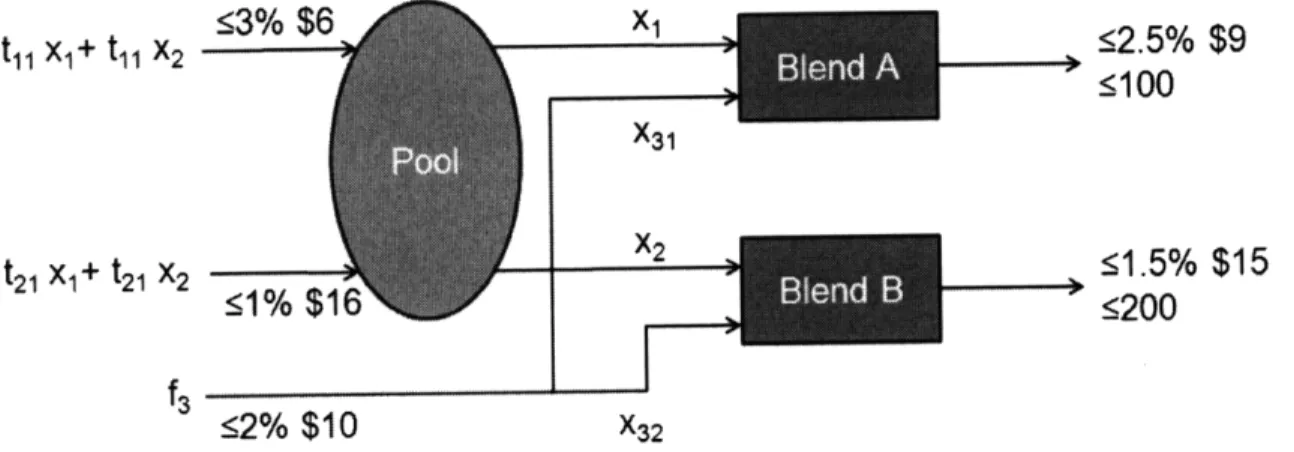
by Ben-Tal et al. (1994) [6] which is called the q-formulation. Ben-Tal et al. (1994) [6]

derives the q-formulation of the pooling problem by introducing new variables tijsatisfying

the relationship:

fj

It can be easily shown that the p- and q-formulations are equivalent. However, the main

advantage of the q-formulation is that, in many applications, the number of extreme points

of the simplex containing the variables tij is much smaller than the number of extreme

points of the hypercube qjw. This advantage is exploited algorithmically by Ben-Tal et al.

(1994) [6]. Figure 2-3 shows the q-formulation of the Haverly's pooling problem.

13% $6

x,

t1

<2.5%

$9

5100

$15

5200

Figure 2-3: The q-formulation of the Haverly's pooling problem

B

Tawarmalani & Sahinidis (2002) [45] constructs the pq-formulation by adding the

fol-lowing constraint to the q-formulation:

1

tijxjk= xjk, j= 1,...,p; k

=

i= 1

Figure 2-4 illustrates the pq-formulation of the Haverly's pooling problem. As can be

realized from this example, the newly added constraints are redundant and don't change the

feasible region. However, the main point of interest in the pq-formulation is the tightness

of the convex relaxations relative to the other two formulations. Tawarmalani&Sahinidis

(2002) [45] prove that the pq-formulation provides much tighter convex relaxations

com-pared to the p- and q-formulations.

<3% $6 x

til x1+ t x2

3

-<1% $16

<2.5%

$9

<100

51.5%

$15

<200

S

B

BlendB

f3

._J

Convexification Const.:

"2% $10

x

x~

t

X

Figure 2-4: The pq-formulation of the Haverly's pooling problem

Tawarmalani & Sahinidis (2002) [45] claim that for all example pooling problems, the pq-formulation decreases solution times drastically and solution times of example pooling problems (solved with BARON) presented in [45] to prove this statement. However, in [45] the chart provided for comparison of three formulations in terms of solution times does feature solutions from different references and therefore with different processors and hence the validity of their claims can be questioned. Therefore, it is decided to model three example pooling problems (Haverly's [18], Foulds' [12] and Adhya's [1]) with all

Table 2.2: Solution times for onds). Problem Haverly Foulds Adhya the p-,q-p- q- pq-0.02 0.016 0.01 1.89 1.46 1.25 9.27 7.71 6.12

and pq- formulations in example problems (in

sec-three different formulations, and these sec-three example problems are solved in GAMS 22.5 [13] with BARON 7.8 [42] used as the global optimization solver. When comparisons are done with a computer having Intel 3.20 GHz Xeon processor, results show that the solution times do not differ immensely as presented in Table 2.2. But still the pq-formulation has the lowest solution times, hence the pq-formulation is featured in this study to formulate the pooling problems to be solved.

Chapter 3

Literature Review

3.1 Deterministic Pooling Problem

Various optimization procedures for the pooling problem have been proposed in the liter-ature. These solution procedures can be classified based on their convergence to either a local or a global optimum. The first algorithm for the pooling problem was suggested by Haverly (1978-1979) [19, 20]. Haverly's approach was based on the idea of using recursion to solve the pooling problem. A recursive approach guesses the value of the pool qualities. These values for the pool qualities converts the pooling problem into a linear program in the flow variables. The actual values of the pool qualities can then be calculated from the values of the flow variables that are obtained by solving the linear program. The process continues until the actual values of the qualities are within a range of tolerance from the guessed values. The main drawback in using any form of recursive method for the pooling problem is that often the algorithm does not converge to a solution, and when it converges, it converges only to a local minimum, a local maximum, or even a non-KKT point. In addi-tion, as the number of pools and end-products increases, recursive methods tend to become more unstable, resulting in computational difficulties.

Successive Linear Programming (SLP) approaches which solve nonlinear problems as

a sequence of linear programs are also widely used. Lasdon (1979) [31] proposes an al-gorithm based on SLP technique. These approaches also do not guarantee global optimal solutions and may converge to even a non-KKT point.

As in the case of GBD, decomposition methods are based on the observation that a dif-ficult problem can be converted to an easier problem by fixing values of certain variables. In the case of the pooling problem, for example, fixing the pool quality variables converts it into a linear program. By using this approach, Floudas & Aggarwal (1990) [11] sug-gest an algorithm based on fixing the pool quality variables as the complicating variables and decomposing the original pooling problem into a primal problem and a relaxed master problem and iterating between these problems based on the GBD algorithm until the termi-nation conditions are satisfied. Although their decomposition strategy is successful for the problems suggested by Haverly, in general it offers no guarantee for global optimality. This GBD algorithm may converge to a local minimum, a local maximum, or even a non-KKT point. Visweswaran & Floudas (1996) [50] propose a GOP algorithm for solving the pool-ing problem. The algorithm was proven to terminate finitely with a global optimum. Uspool-ing this algorithm, the authors were able to solve three cases of the Haverly problem. It is also reported that a single pool, five-product problem, with each stream having two quality components is solved to global optimality using this algorithm. Large-scale pooling prob-lems, generated randomly, having up to 5 pools, 5 products, and 30 qualities, were solved by Androulakis et al. (1996) [2] using a different implementation of the GOP algorithm.

Branch-and-bound (B+B) methods for pooling and blending problems have been sug-gested by different authors. These methods usually differ in the relaxations used to provide valid lower bounds to the global optimum. Foulds et al. (1992) [12] use a procedure which involves replacing the bilinear terms in the pooling problem by their McCormick (1983) [35] concave and convex envelopes. The nonlinear pooling problem can be relaxed to a linear programming problem, the solution of which provides a lower bound on the global optimal solution. The B+B procedure proceeds by partitioning the feasible set and relaxing

on each partition. It is quite obvious that by replacing each bilinear term by its concave or convex envelope introduces a relaxation, but this relaxation also tends to zero as the partitions get finer and the algorithm converges to the global optimal solution. Using this approach, Foulds et al. (1992) [12] were able to solve single-quality problems, with the largest problem having 8 pools and 14 products. The constraints which provide the convex and concave envelopes of the problem at a specific node of the B+B tree are not in general valid for other nodes of the tree. Thus, the convex and concave envelopes have to be gener-ated at each node of the B+B tree. However, the McCormick relaxation requires four linear constraints to provide the envelopes for each bilinear term in the problem. Hence, as the number of pools, products, or component qualities increase, the size of the linear program to be solved at each node of the B+B tree also increases.

Ben-Tal et al. (1994) [6] propose another lower-bounding procedure based on La-grangian relaxation of another formulation of the pooling problem (explained in the pre-vious chapter as the q-formulation). In this paper, a B+B algorithm which partitions the feasible set of the pooling problem is provided and it is shown that this approach can reduce the duality gap between a nonconvex problem and its dual. Later it is also proven that for partially convex problems such as the pooling problem, under certain regularity conditions, this approach can reduce the duality gap between the primal and the dual to zero.

Adhya et al. (1999) [1] use yet another formulation of the pooling problem (explained in the previous chapter as the pq-formulation). The authors provide a new Lagrangian relaxation approach for developing lower bounds for the B+B to solve the pooling problem and it is proven that the Lagrangian relaxation approach provides tighter lower bounds than the standard linear-programming relaxations used in global optimization algorithms and hence guarantees faster convergence speeds.

3.2 Infrastructure Development and the Stochastic

Pool-ing Problem

For the infrastructure development problem, most of the literature is on oil production planning and unfortunately there is only small amount of literature dealing specifically with natural gas production planning, but usually modeling and solution strategies for oil and gas infrastructure development problems are very similar. Hence, no distinction is made between the oil and gas production planning literature, and the literature for oil production planning is also included to this review.

Most of the available literature for planning of oil and gas field infrastructures uses a de-terministic approach without considering how uncertainty affects the overall system (Iyer, Grossmann, Vasantharajan & Cullick (1998) [22]; Van den Heever & Grossmann (2000) [47]; Van den Heever & Grossmann (2001) [48]; Barnes, Linke & Kokossis (2002) [4]; Lin & Floudas (2003) [32]; Ortiz-Gomez, Rico-Ramirez & Hernandez-Castro (2002) [37]). For a recent review of the existing literature on deterministic approaches for these problems, re-fer to Van den Heever & Grossmann (2001) [48]. Recently, there has been some work that considers uncertainty in the infrastructure development problem. Jonsbraten (1998) [24] presents an MILP model for optimizing the investment and operation decisions for an oil-field under uncertainty in oil prices. The author uses the Progressive Hedging Algorithm to solve the problem. Jonsbraten (1998ii) [25] presents an implicit enumeration algorithm for the sequencing of oil wells under uncertainty in oil reserves. The decision models for both these papers include investment and operational decisions for one field only. Jornsten (1992) [27] uses Lagrangian relaxation of constraints to solve a stochastic program for the sequencing of gas fields under uncertainty in future demands. The author assumes that production profiles and capacities of platforms have already been fixed. Haugen (1996) [18] proposes a single parameter representation for uncertainty in the size of reserves and incorporates it into a Stochastic Dynamic Programming model for scheduling of petroleum

fields. This work also assumes that the only decisions that need to be made are regarding the scheduling of fields. Meister, Clark, and Shah (1996) [36] present a model to derive exploration and production strategies for one field under uncertainty in reserves and future oil price. The model is analyzed using stochastic control techniques. Lund (2000) [33] presents a stochastic dynamic programming model for evaluating the value of flexibility in offshore development projects under uncertainty in future oil prices and in the reserves of one field. Jonsbraten (1998iii) [26] discusses an interesting problem dealing with planning of oil field development. A situation is considered where two surface lease owners with access to the same oil reservoir bargain their shares of production. The author assumes a mixed-integer optimization model and uses game theory. Recently, there has also been some work using real options based approaches (Dias, 2001 [9]) for planning of oil and gas field developments under uncertainty.

Based on the dependence of the stochastic process on the decisions, Jonsbraten (2001) [27] and Goel & Grossmann (2004) [15] classify uncertainty in planning problems into two categories: project exogenous uncertainty and project endogenous uncertainty. Prob-lems where the stochastic process is independent of the project decisions are said to have project exogenous uncertainty. For these problems, the scenario tree is fixed and does not depend on the decisions. Hence the most relevant characteristic of this kind of stochastic programming model is that its formulation assumes a given scenario tree. The uncertainty in gas prices in a planning problem similar to the one described here is an example of project exogenous uncertainty. For recent reviews on models and solution techniques for stochastic programs with project exogenous uncertainty, please refer to Kall and Wallace (1994) [29] and Birge and Louveaux (1997) [7]. Problems where the project decisions in-fluence the stochastic process are said to possess project endogenous uncertainty. A gas production planning problem with uncertainty in gas reserves is included in this category. This is because the uncertainty in gas reserves of a field is resolved only if, and when, exploration or investment is done at the field. If no action is taken, the uncertainty in the

field does not resolve at all. For problems with project endogenous uncertainty, the sce-nario trees are decision-dependent. This leads to difficulties in defining the model because, traditionally, the stochastic programming literature has relied on the assumption of given scenario trees. Hence, there is very little literature dealing with problems having process endogenous uncertainty. An intensive literature search provides only four papers (Pflug, (1990) [38]; Jonsbraten, Wets & Woodruff, (1998) [24]; Jonsbraten, (1998ii) [25]; Goel & Grossmann, (2004) [15]) which deal with project endogenous uncertainty.

A Literature review clearly shows that none of the literature about the infrastructure development problem considers the concentrations of the impurities in the natural gas pro-duced as a source of uncertainty, but as mentioned in the first chapter, because of the con-tractual agreements, regulations and the pipeline requirements, the production company has to adjust the composition of the gas within some limits to sell it, and the composition of gas is unknown when infrastructure is being developed. To blend gas from different fields, while the infrastructure is being developed, the pipeline system has to be constructed to allow the gas from different wells to be mixed to satisfy the requirements. Therefore, to develop the value chain optimally, a stochastic version of the pooling problem where the quality parameters in the wells are unknown has to be solved. Therefore, gas quality un-certainty in the infrastructure development problem is selected in this study as the first step to construct and solve a realistic model of the whole infrastructure development problem with more realistic or less assumptions than the literature until now.

Another important assumption in the literature is that the effect of the contractual frame-work is not considered. However, in most fields natural gas cannot be produced unless a contractual demand exists and in addition the rules given in contracts and also in govern-mental regulations need to be taken into account to reach a realistic model of the system. In addition, there are other important assumptions: no expansion in capacity of a platform is considered; in most of the references production rate decreases linearly in time; flow mod-els and reservoir modmod-els are assumed as linear and more importantly effects of contractual

Chapter 4

BD Algorithm for Deterministic Pooling

Problem

4.1

Introduction of Benders Decomposition Algorithm

The Benders Decomposition algorithm was originally proposed by Benders in 1962 [5] for nonlinear, nonconvex mixed variables programming problems of the form:

max _{cTx + f(y)} (4.1)

s.t. Ax+F(y) < 0 (4.2)

x EXC Rn

x,y EU C n y

where y is a vector of complicating variables, since the problem above can be solved more easily when y is fixed constant. In other words, for fixed y, this problem separates into a number of smaller problems each having only subsets of x as variable or the problem assumes a special structure, such as a linear program as in the case of the pooling problem

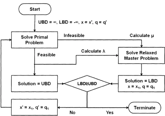
or the problem is converted into a convex program. In these cases, by fixing y, a simpler primal problem can be solved and a relaxed master problem is solved to generate valid lower bounds and the algorithm converges to the global optimum by iterating between these problems. In practice, the BD algorithm decomposes problem into two smaller problems: primal problem (linear program) and relaxed master problem (nonlinear program in bilinear problems). The primal problem is used to find the upper bound (UBD); the relaxed master problem is used to find the lower bound (LBD). When LBD>UBD, algorithm terminates.

On the other hand, the Generalized Benders Decomposition algorithm is first proposed by Geoffrion (1972) [14] and also based on Benders Decomposition, but it is proposed to solve more general form of nonconvex nonlinear programs of the form:

max f(x,y) (4.3)

xy

s.t. g(x,y) < 0 (4.4)

x EX C Rnx,y E U C Rn y

where y is a vector of complicating variables, again, in the sense that it is much easier to solve in x when y are held fixed. However, the problem to be solved has to satisfy a property called "Property P", unlike Benders Decomposition. Basically, the problem to be solved has to be formulated such that for every X > 0, (where Xs are the Lagrange multipliers), the infimum of f (x,y) + , Tg(x,y)) over X can be taken essentially independently of y, so that the constraints in the relaxed master problem can be obtained explicitly with little or no more effort than is required to evaluate it at a single value of y.

As it is known, bilinear terms are formed by the multiplication of two variables of the problem and these bilinear terms introduce nonconvexities to the problem. If the noncon-vexities in the problem are only introduced by the bilinear terms, as in the case of pooling

problems, it is possible to treat the whole bilinear terms as a complicating variable in the BD algorithm as opposed to fixing only one of the variables in bilinear terms as the com-plicating variable. Fixing the bilinear terms yields constant parameters. Then, the general formulation of the pooling problem can be written (consistently to the notation given in

Chapter 2) as:

max cTf + dTy (4.5)

s.t. Af + F(y) 0 (4.6)

f E F c Rf,y

E

where c is the cost vector, d is the price vector, f is the input flow vector and y is the vector for the bilinear terms which is equal to qTx (q is the vector of quality variables and

x is the vector for flow from the pools to demands as explained in Chapter 2).

Therefore, the BD algorithm can be applied to pooling problems and is guaranteed to converge to the global optimum (as proved in the next section) when both of the bilinear terms are taken as the complicating variables. Obviously, in the BD implementation, the primal problem becomes a linear program which is obviously convex and the relaxed mas-ter problem is a nonconvex NLP where a global solver such as BARON can be used to obtain global optimal solutions. Using these global optimal solutions to iterate, it is pos-sible to generate valid cuts that converge. Hence, this approach is expected to converge to the global optimum of the pooling problem with Benders Decomposition reliably.

Then, for instance, in Haverly's pooling problem, the primal problem can be formulated

as:

min 6fi +1 16f2 + 10fl2-9 x + 2 1 -15 x1 2 +x2 2) (4.7)

s.t.

fii

f12 - X21 - X22 = 0 (4.9)

q' (Xl+XX2) -3fiI -f21 =0 (4.10)

qxll +x21 -2.5 xl I +X21 ) 0 (4.11)

qx2

+

+

where q, xl₁ and xl2 are constant parameters which are assigned as the fixed compli-cated variables. Therefore, bilinearities in the primal problem disappear and it becomes a linear program and therefore, it is convex. However, the relaxed master problem is still a bilinear program and it is obviously a nonconvex NLP. Hence, still the relaxed master problem has to be solved with a global solver such as BARON. But, the potential benefit of utilizing BD algorithm might be to solve number of smaller problems (the relaxed master problems) with the B+B procedure (such as BARON) instead of solving one huge prob-lem with the B+B. B+B _{based algorithms are exponential-time algorithms. In other words,}

as the problem size increases, solution times of B+B algorithms increases exponentially. Therefore, instead of solving a problem with large number of variables, solving number of problems with small number of variables can be quicker in terms of the solution times.

As mentioned, the primal problem becomes a linear program and general formulation of the primal problem becomes:

p r p min cijfij- dk Xjk f ,x j=1 iNj k=1 j=l r s.t. fij- xjk = 0 j= 1,. ieNj k= 1 r qw Xjk k=l (4.13) (4.14) (4.15) I

,ijwfij = 0,

where qi, Xjk are the fixed parameters. And as it is seen, also in a general pooling problem formulation, the primal problem is a linear program and therefore, it is convex.

In addition, the relaxed master problem can be formulated as: R: min n1 s.t. 71 > inf(F + T _g i) W'gi < 0O (4.18) (4.19) (4.20)

where 2X is the vector of Lagrange multipliers, y is the vector of multipliers for the feasibility problem, F is the objective function and gi are the constraint functions, which

j=

=

k= 1,...,r

k= 1,...,r; w = 1,...,

means: p r p F = cijfij- dk xjk (4.21) j= 1 iENj k=l j=l r gl =

fi-

j

Then, the proposed BD algorithm for pooling problems is presented in Algorithm I and also flowchart of the algorithm is provided in Figure 4-1. As Figure 4-1 represents, basically, The primal problem provides the upper bound value (UBD) whereas the relaxed master problem provides the lower bound value (LBD) and when LBD>UBD, algorithm terminates.

By using this algorithm, different pooling problems from the literature are solved and validity and speed of this approach is tested versus algorithms which guarantees global optimal solution such as BARON. However, before testing the algorithm, the first step is to prove its convergence to global optimum.

4.2

Proof of Convergence

To prove the convergence of the proposed algorithm, the first step is to show that the pooling problem formulation satisfies the form given by Benders (1962) [5]:

Algorithm 1 Benders decomposition algorithm for global solution of pooling problems

{ INITIALIZATION }

i (iteration) := 1, UBD := INF, LBD := -INF, p := 0, r := 0;

Select an initial configuration for the variables: q (i) = q' (i) and x (i) = x' (i)

{STEP 1: LP PRIMAL PROBLEM}

Solve Problem (P) with q (i) = q' (i) and x (i) = x' (i),

{FEASIBLE PRIMAL}

if Problem (P) with q (i) = q (i) and x (i) = x' (i) is feasible then,

Let the solution be f* (i), let p = p+l and = P. (, is the corresponding duality multi-X plier.)

if z* (i) < UBD then, (where z* (i) is obj. value of the LP Primal Problem at iteration i.)

{RECORD BETTER SOLUTION}

UBD := z* (i), x* := x' (i),f* := f* (i), q*:= q' (i). end if

{INFEASIBLE PRIMAL}

if Problem (P) with q (i)

=

=

=

{STEP 2: NLP RELAXED MASTER PROBLEM}

ifp=O then, solve the feasibility version of the NLP Master Problem. else, solve min 1r x,q,17 s.t > inf(h(f,x)+ (i gi(fx,q)), Vj = 1,...,p x,q (P )T gi(f,x, q)

< 0,

r

where h(fx) is the objective function and gi(f,x,q) are the constraints.

Let the solution be qmp (i) and xmp (i), then q' (i + 1) = qmp (i) and x' (i + 1) = xmp (i). end

if

if 7r_* > LBD then,

{RECORD BETTER SOLUTION}

LBD := l* (i). end if if LBD > UBD then, STOP. else, i := i+l, Go to STEP 1. end if

o, LBD = -o, x = x', q= q'

Figure 4-1: Flowchart of the proposed BD algorithm

max _{c x + f(y)}

s.t. Ax+F(y)<O

(4.26)

(4.27)

x EX C Rn ,y E U C Rny

Then, the convergence can be directly proved from Benders (1962). The pooling prob-lem in Chapter 2 can be reformulated as:

max

xf cTf + dTx (4.28)

f

Q

The crucial point in satisfying Benders (1962) [5] formulation and hence proving con-vergence is when the complicating variables are fixed, the resulting formulation has to be a linear program. Since in the proposed algorithm both x and q (bilinear terms) are fixed as complicating variables. The resulting formulation in the pooling problem is:

max cTf + B (4.30)

x,f

s.t. Af+C<O (4.31)

fe FC Rn,

where B = dT, C = F(x, q-) and xand q-are fixed parameters. It is obvious that the re-sulting formulation is a linear program and hence it can be concluded that proof of conver-gence for the proposed BD algorithm can be derived directly from the proof of converconver-gence of Benders original algorithm.

Benders (1962) [5] states that the problem given in the form of (4.28) and (4.29) can be written in the equivalent form by introducing a scalar variable fo:

max {fo fo-cTf - dTx<0 O, Af +F(x,q) < O0,x > 0} (4.32)

In other words, (fo,f,-,q) is an optimum solution of problem if and only if fo =

cTf+ dTy and (f x, q is an optimum solution of the problem.

Theorem 3.1 (Partitioning Theorem for mixed-variables) of Benders (1962) [5] proves that (a) (f, , q) is an optimum solution of problem denoted by (4.29) and (4.30) if and only

if (fo,fx, q) is an optimum solution of (4.33). In addition, this theorem shows that (b) if 47