Deep learning in event-based neuromorphic systems

HAL Id: tel-02417462

https://tel.archives-ouvertes.fr/tel-02417462

HAL is a multi-disciplinary open access archive for the deposit and dissemination of sci-entific research documents, whether they are pub-lished or not. The documents may come from teaching and research institutions in France or abroad, or from public or private research centers.

L’archive ouverte pluridisciplinaire HAL, est destinée au dépôt et à la diffusion de documents scientifiques de niveau recherche, publiés ou non, émanant des établissements d’enseignement et de recherche français ou étrangers, des laboratoires publics ou privés.

To cite this version:

Johannes C. Thiele. Deep learning in event-based neuromorphic systems. Artificial Intelligence [cs.AI]. Université Paris Saclay (COmUE), 2019. English. �NNT : 2019SACLS403�. �tel-02417462�

Th

`ese

de

doctor

at

NNT

:2019SA

CLS403

Neuromorphic Systems

Th`ese de doctorat de l’Universit´e Paris-Saclay pr´epar´ee `a l’Universit´e Paris-Sud Ecole doctorale n◦₅₇₅

Electrical, Optical, Bio : PHYSICS-AND-ENGINEERING (EOBE)

Sp´ecialit´e de doctorat : Sciences de l’information et de la communication

Th`ese pr´esent´ee et soutenue `a Palaiseau, le 22.11.2019, par

J

C

T

Composition du Jury : Antoine Manzanera

Enseignant-Chercheur, ENSTA ParisTech Pr´esident Simon Thorpe

Directeur de Recherche, CNRS Rapporteur Shih-Chii Liu

Privatdozent, ETH Zurich Rapporteur Emre Neftci

Assitant Professor, UC Irvine Examinateur Antoine Dupret

Ing´enieur-Chercheur, CEA/LIST Directeur de th`ese Olivier Bichler

This thesis was hosted by the DACLE department of CEA, LIST. I want to thank Thierry Collette, the former head of the department, and the current head Jean Ren´e Lequepeys, for offering me the possibility to perform my doctoral project in their department. I want to thank all members of the CEA laboratories that hosted me during my thesis, LCE and L3A, and their respec-tive heads Nicolas Ventroux and Thomas Dombek, for the great personal and scientific support they offered me throughout the whole duration of my doc-torate. In particular, I want to express my gratitude towards all members of the neural network group, for answering a physicist his many questions about software design and hardware. It was a great pleasure to work together with all of you and I am happy to be able to continue with our excellent work in the years to come. I am grateful for your great patience and support in those months when I was still getting accustomed to the French language.

Most of all, I want to thank my supervisors Olivier Bichler and Antoine Dupret for supporting me with their extensive technical knowledge and re-search experience. I am grateful for their great trust in me and the autonomy they offered me during my thesis, while always being present to answer my questions with great patience and expertise.

I want to thank all jury members for studying my manuscript and par-ticipating in my defense. In particular, I want to thank my thesis reviewers Shih-Chii Liu and Simon Thorpe for providing me such precise and helpful feedback on my manuscript. Many thanks to Antoine Manzanera and Emre Neftci for participating as jury members in my defense.

I also want to thank our collaborators at INI in Zurich for our productive work, in particular Giacomo Indiveri for offering me the opportunity to spend time in his research group during my thesis.

Finally, I want to thank all my loved ones for supporting me during my doctorate. In particular, I want to express my gratitude towards my parents Walter and Elvira Thiele, for enabling me to pursue my studies for all of these years, up to this final academic degree.

Résumé en français

Les réseaux de neurones profonds jouent aujourd’hui un rôle de plus en plus important dans de nombreux systèmes intelligents. En particulier pour les applications de reconnaissance des objets et de traduction automatique, les réseaux profonds, dits «deep neural networks», représentent l’état de l’art. Cependant, inférence et apprentissage dans les réseaux de neurones profonds nécessitent une grande quantité de calcul, qui dans beaucoup de cas limite l’intégration des réseaux profonds dans les environnements en ressources li-mitées. Étant donné que le cerveau humain est capable d’accomplir des tâches complexes avec un budget énergétique très restreint, cela pose la question si on ne pourrait pas améliorer l’efficacité des réseaux de neurones artificiels en imitant certains aspects des réseaux biologiques. Les réseaux de neurones évènementiels de type «spiking neural network (SNN)», qui sont inspirés par le paradigme de communication d’information dans le cerveau, représentent une alternative aux réseaux de neurones artificiels classiques. Au lieu de pro-pager des nombres réels, ce type de réseau utilise des signaux binaires, appel-lés «spikes», qui sont des évènements déclenchés en fonction des entrées du réseau. Contrairement aux réseaux classiques, pour lequels la quantité de cal-cul effectué est indépendante des informations reçues, ce type de réseau évè-nementiel est capable de traiter des informations en fonction de leur quantité. Cette caractéristique entraine qu’une grande partie d’un réseau évènemen-tiel restera inactif en fonction des données. Malgré ces avantages potenévènemen-tiels, entraîner les réseaux spike reste un défi. Dans la plupart des cas, un réseau spike, pour une même architecture, n’est pas capable de fournir une préci-sion d’inférence égale au réseau artificiel classique. Cela est particulièrement vrai dans les cas où l’apprentissage doit être exécuté sur un matériel de calcul bio-inspiré, dit matériel neuromorphique. Cette thèse présente une étude sur les algorithmes d’apprentissage et le codage d’informations dans les réseaux de neurones évènementiels, en mettant un accent sur les algorithmes qui sont capables d’un apprentissage sur une puce neuromorphique. Nous commen-çons notre étude par la conception d’une architecture optimisée pour

l’ap-entre-carte

Figure 0.1: Structure basique d’une couche convolutive avec inhibition WTA entre-carte et intra-entre-carte. Chaque entre-carte de charactéristiques (montrées en différentes cou-leurs) détecte des charactéristiques dans l’image entière. Si un neurone déclenche un évènement, tous les neurones des autres couches, se trouvant au voisinage du neu-rone déchlenché, sont inhibés, de même que les neuneu-rones de la carte du neuneu-rone déchlenché.

prentissage continu, qui apprend avec une règle d’apprentissage type STDP («spike-timing dependent plasticity», littéralement plasticité dépendant de l’ins-tant de déclenchement). Le STDP est une règle d’apprentissage non-supervisée qui permet, avec un mécanisme compétitif du type WTA («winner-takes-all», littéralement le vainqueur prend tout), une extraction des caractéristiques des données non-étiquettées (figure 0.7). Cette règle est facilement réalisable dans les matériels neuromorphiques. Ce mécanisme d’apprentissage nous permet de construire un système capable d’un apprentissage interne dans une puce neuromorphique, potentiellement avec une haute efficacité énergétique. Cette approche est utilisée pour l’apprentissage des caractéristiques dans un CNN («convolutional neural network», réseau de neurones convolutif). Ce réseau consiste en deux couches convolutives, deux couches de «pooling»(qui re-groupent les entrées en faisant la moyenne d’une région spatiale) et une couche entièrement connectée. Dans les approches précédentes, le mécanisme de WTA permettait seulement une apprentissage couche par couche. En utili-sant un modèle de neurone avec deux accumulateur (figure 0.2), nous sommes capables d’entraîner toutes les couches du réseau simultanément. Ce modèle de neurone représente une caractéristique innovante de notre architecture, qui facilite largement l’apprentissage continu. De plus, nous montrons que le choix spécifique de la règle STDP, qui mesure les temps d’évènements en fonc-tion des dernières remises à zéro et qui n’utilise que des temps absolus,

per-Θinf entrée synaptique STDP évènement (c) ΘWTA remise à zéro

Figure 0.2: (a) Description schématique du neurone en deux accumulateurs. Le neu-rone intègre tous les entrées reçues simultanément dans deux accumulateurs, l’un pour le déclenchement STDP et WTA, l’autre pour l’inférence (cela veut dire la propa-gation d’évènements).(b) Interaction entre deux neurones liés par inhibition latérale. Si l’intégration d’accumulateur WTA dépasse le seuil, aucun évènement n’est propagé à la couche suivante. Cependant, le neurone déclenche STDP et l’inhibition latérale, qui remet à zéro les intégrations des autres neurones. (c) Si l’intégration dépasse le seuil dans l’accumulateur d’inférence, un évènement est propagé et l’intégration est remise à zéro. Les accumulateurs d’inférence des autres neurones restent inaffectés, ou sont alternativement influencés par une inhibition de courte distance (plus courte que l’inhibition des accumulateurs d’apprentissage). Cela permet de contrôler com-bien de cartes par position contribuent à la propagation des évènements.

met d’obtenir une invariance temporelle de fonctionnement du réseau. Nous montrons que notre architecture est capable d’une extraction des caractéris-tiques pertinentes (figure 0.3), qui permettent une classification des images des chiffres de la base de données MNIST. La classification est faite avec une simple couche entièrement connectée dont les neurones correspondent aux prototypes des chiffres. Notre architecture démontre une meilleure perfor-mance de classification que les réseaux de l’état de l’art qui consistent seule-ment en une couche entièreseule-ment connectée, qui montre l’avantage de passer des informations par des couches convolutives. On parvient à une précision de classification maximale de 96, 58%, qui est la meilleure précision pour un réseau où toutes les couches sont entrainées avec un mécanisme STDP. Nous montrons la robustesse du réseau face aux variations du taux d’apprentissage et le temps de présentation des stimuli. En changeant la taille des différentes couches du réseau, nous montrons que la performance du réseau peut être améliorée en augmentant le nombre des neurones dans la couche entièrement

férences de contraste locales. Les caractéristiques du haut niveau sont construites en choisissant pour chaque neurone la caractéristique de la couche précédente avec le poids le plus fort. Parce que les filtres dans des positions différentes se chevauchent, les caractéristiques ont une apparence floue. On voit que dans la deuxième couche convolutive, les neurones deviennent sensibles aux parties de chiffres. Finalement, dans la couche entièrement connectée, chaque neurone a appris une caractéristique qui ressemble à un prototype spécifique d’un chiffre faisant partie d’une des diffé-rentes classes (chiffre de 0 à 9 de gauche à droite).

connectée et la deuxième couche convolutive. Comme extension de ces tra-vaux, nous montrons que le réseau peut aussi être appliqué à l’apprentissage des caractéristiques d’une base de données dynamique, N-MNIST, qui repré-sente une version de MNIST avec des chiffres en mouvement. Avec quelques changements mineurs des paramètres de notre architecture, il est capable d’apprendre des caractéristiques qui maintiennent l’information du mouve-ment (figure 0.4). En ajoutant une deuxième couche entièremouve-ment connectée avec un classificateur supervisé, nous sommes capables d’obtenir une préci-sion de classification de 95, 77%. Cela représente la première démonstration d’un apprentissage de N-MNIST dans un réseau convolutif où toutes les ca-ractéristiques sont apprises par un mécanisme STDP. Nous montrons égale-ment que l’architecture est capable d’une inférence basée seuleégale-ment sur des sous-mouvement. Nos résultats montrent alors que notre architecture pos-sède toutes les capacités nécessaires pour un système neuromorphique qui doit effectuer un apprentissage sur un flux de données évènementielles.

En comparaison avec des approches supervisées fondées sur l’algorithme BP («backpropagation», la rétro-propagation du gradient), notre architecture démontre une performance de classification inférieure. Nous présentons une analyse des différents algorithmes d’apprentissage pour les réseaux spike d’un point de vue localité de l’information. Reposant sur cette synthèse, nous expliquons que les règle d’apprentissage du type STDP, qui sont spatialement et temporellement locales, sont limitées dans leur capacité d’apprendre cer-taines caractéristiques nécessitant une optimisation globale du réseau. Cette

faiblesse pourrait expliquer leurs performances inférieures par rapport aux mécanismes d’optimisation non-locaux type rétro-propagation du gradient.

Pour dépasser ces limites du STDP, nous élaborons un nouvel outil pour l’apprentissage dans les réseaux spike, SpikeGrad, qui représente une implé-mentation entièrement évènementielle de la rétro-propagation du gradient. Cet algorithme est construit à partir d’un modèle de neurone spécial possé-dant un deuxième accumulateur pour l’intégration des informations du gra-dient. Cet accumulateur est mis à jour d’une manière pratiquement équiva-lente à l’accumulateur ordinaire du neurone, avec la différence que la dérivée de la fonction d’activation est prise en compte pour le calcul du gradient. En utilisant un accumulateur d’activation de neurone qui est pondéré par le taux d’apprentissage, SpikeGrad est capable d’effectuer un apprentissage qui repose uniquement sur des accumulations et des comparaisons. De plus, Spi-keGrad possède un autre grand avantage. En utilisant un modèle de neurone type IF («integrate-and-fire», littéralement intègre-et-déclenche) avec une fonc-tion d’activafonc-tion résiduelle, nous montrons que les activafonc-tions accumulées des neurones sont équivalentes à celles d’un réseau de neurones artificiels. Cela permet la simulation de l’apprentissage du réseau évènementiel en tant que réseau de neurones artificiels classique, qui est facile à effectuer avec le ma-tériel de calcul haute performance typiquement utilisé dans l’apprentissage profond.

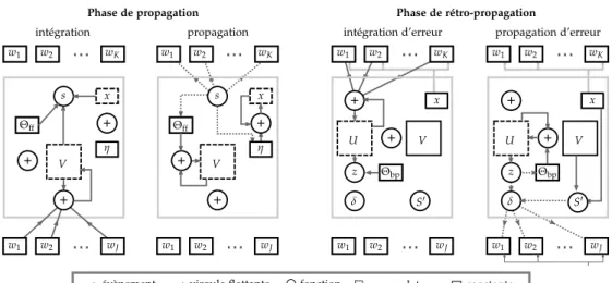
l’entraine-x V w1 w2 wJ U V x S0 δ z Θbp x η s Θff Θff V η s V U x δ z Θbp S0

évènement virgule flottante fonction accumulateur constante

w1 w2 wJ w1 w2 wJ w1 w2 wJ

Figure 0.5: Phases de propagation et rétro-propagation dans un seul neurone dans l’algorithme SpikeGrad. Intégration : Chaque fois qu’un signal évènementiel arrive à une des synapses{w1, ..., wJ}, la valeur du poid est ajoutée à la variable

d’intégra-tion V ponderée par le signe de l’évènement. Après chaque mise à jour, la variable d’intégration est comparée au seuil_±Θ_ffet la trace synaptique x par la fonction d’ac-tivation évènementielle s, qui décide si un évènement sera déclenché. Propagation : Si un évènement est déclenché, il augmente la trace x par le taux d’apprentissage±η, et

il est transmis aux connexions sortantes. L’intégration est augmentée par_±Θ_ffselon le signe de l’évènement. Intégration d’erreur : Des évènements signés sont reçus par les synapses{w1, ..., wK}des connexions sortantes. La valeur du poid est ajoutée à la

variable d’intégration d’erreur U, et elle est comparée au seuil_±Θ_bp par la fonction z. Propagation d’erreur : Si le seuil est dépassé, un évènement signé est émis et U est incrémentée par±Θbp. L’évènement est pondéré par la dérivée de la fonction

d’ac-tivation effective (qui est calculée avec V et x), et propagé à travers les connexions entrantes. Les poids des neurones sont mis à jour en utilisant ce signal d’erreur et les traces synaptiques des neurones de la couche précédente.

ment d’un réseau spike qui est capable d’inférer des relations entre des va-leurs numériques et des images. Notre première démonstration concerne un réseau qui apprend la relation A+B=C. Nous montrons que SpikeGrad per-met d’entraîner ce type de réseau plus rapidement, avec moins de neurones, et avec une meilleure précision d’inférence que les approches bio-inspirés de l’état de l’art. La deuxième tache examinée est l’apprentissage d’une version visuelle de la relation logique XOR, sur les images de 0 et 1 de MNIST. Nous montrons également que le réseau est capable d’une inférence visuelle dans ce scenario, et qu’il peut produire des stimuli artificiels qui ressemblent aux exemples qu’il a reçus pendant l’apprentissage.

La deuxième démonstration des capacités de SpikeGrad est faite sur une tâche de classification. Il est montré que l’outil est capable d’entraîner un

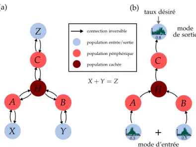
X+Y=Z 0.5 0.3 A B C H population périphérique population entrée/sortie A B C H 0.8 mode d’entrée mode de sortie connection inversible Z Y X population cachée

Figure 0.6: (a) Architecture du réseaux relationnel avec trois variables. Les popula-tions d’entrée/sortie sont marquées par X, Y, Z. Les populapopula-tions périphériques sont marquées par A, B, C, et la population cachée par H. (b) Entraînement du réseau. Pendant l’apprentissage, deux populations servent comme populations d’entrée et fournissent un profil des taux de déclenchement désiré. La troisième population est entraînée pour reproduire ce profil, à partir des entrées. Ces différents rôles des po-pulations sont interchangés pendant l’apprentissage pour permettre une inférence dans tous les sens de la relation.

Y 0.0 0.2 0.4 0.6 0.8 1.0 Z 0.0 0.2 0.4 0.6 0.8 1.0 X 0.0 0.2 0.4 0.6 0.8 1.0 X 0.0 0.2 0.4 0.6 0.8 1.0 Z 0.0 0.2 0.4 0.6 0.8 1.0 Y 0.0 0.2 0.4 0.6 0.8 1.0 X 0.0 0.2 0.4 0.6 0.8 1.0 Y 0.0 0.2 0.4 0.6 0.8 1.0 Z 0.0 0.2 0.4 0.6 0.8 1.0

Figure 0.7: Inférence des trois variables de la relation. Les deux axes du fond marquent les deux variables d’entrée, tandis que l’axe vertical représente la valeur inférée. On voit que le réseau a appris à représenter précisement toutes les directions possibles de la relation.

ressemblent aux autres stimuli de la base de données.

Architecture Méthode Taux Rec. (max[moyen±dev.])

Rueckauer et al. [2017] CNN converti à SNN 99, 44%

Wu et al. [2018b]* SNN entraîné avec BP float. 99, 42%

Jin et al. [2018]* Macro/Micro BP 99, 49%

Ces travaux* SNN entraîné avec BP float. 99, 48[99, 36±0, 06]%

Ces travaux* SNN entraîné avec BP évènementiel 99, 52[99, 38±0, 06]%

Table 0.1: Comparaison des différentes méthodes de l’état de l’art des architectures CNN évènementielles sur MNIST. * marque l’utilisation de la même topologie (28x28-15C5-P2-40C5-P2-300-10).

grand réseau spike convolutif, qui donne des taux de reconnaissance d’image compétitive (figures 0.1 et 0.2). Sur MNIST, nous obtenons une précision de classification de 99, 52%, et sur CIFAR10, nous obtenons 89, 99%. Dans les deux cas, ces précisions sont aussi bonnes que celles des réseaux spike entraî-nés avec la rétro-propagation en virgule flottante. Elles sont aussi comparables avec celles des réseaux de neurones classiques possédant une architecture comparable. De plus, nos résultats montrent que ce type de rétro-propagation évènementielle du gradient pourrait facilement exploiter la grande parcimo-nie qui se trouve dans le calcul du gradient. Particulièrement vers la fin d’ap-prentissage, quand l’erreur commence à diminuer fortement, la quantité de calcul pourrait diminuer fortement en utilisant un codage évènementiel.

Nos travaux introduisent alors plusieurs mécanismes d’apprentissage puis-sants. La première partie de nos travaux avait comme objectif d’utiliser un mécanisme d’apprentissage bio-inspiré pour construire un système neuro-morphique capable d’un apprentissage continue. Pour franchir plusieurs li-mitations de cette approche, nous avons ensuite développé une implémenta-tion évènementielle de la rétro-propagaimplémenta-tion du gradient. Ces approches pour-raient alors promouvoir l’utilisation des réseaux spike pour des problèmes réels. Dans notre opinion, les approches comme SpikeGrad, qui sont basées sur

Wu et al. [2018a]* SNN entraîné avec BP float. (sans «NeuNorm») 89, 32%

Sengupta et al. [2019] SNN (VGG-16) converti à SNN SNN 91, 55%

Ces travaux* SNN entraîné avec BP float. 89.72[89, 38±0, 25]%

Ces travaux* SNN entraîné avec BP évènementiel 89, 99[89, 49±0, 28]%

Table 0.2: Comparaison des différentes méthodes de l’état de l’art des architectures CNN évènementielles sur CIFAR10. * marque l’utilisation de la même topologie (32x32-128C3-256C3-P2-512C3-P2-1024C3-512C3-1024-512-10). Ces travaux (STDP) Année Pr écision [%]

Ces travaux (grad. float.)

Ces travaux (SpikeGrad)

Mozafari et al. [2019] Diehl et Cook [2015] Querlioz et al. [2011] Kheradpisheh et al. [2017] Lee et al. [2016] Neftci et al. [2017] O’Connor et Welling [2016] Diehl et al. [2015] Jin et al. [2018] Rueckauer et al. [2017] BP interne BP externe STDP externe STDP interne

Figure 0.9: Développement des précisions d’inférence de l’état de l’art sur MNIST pendant les dernières années. On voit que les travaux initiaux utilisaient surtout des approches STDP. Alors qu’il y a encore de la recherche sur l’amélioration des performances des SNNs entraînés avec STDP, les meilleurs résultats des dernières années sont fournis par des méthodes qui utilisent des approximations de la rétro-propagation. SpikeGrad est la première méthode pour l’apprentissage interne sur puce qui donne des précisions comparables aux méthodes d’apprentissage externes. Veuillez noter que cette présentation est simplifiée et montre seulement les tendances générales qui sont observables dans la domaine. Surtout, nous n’avons pas pris en compte l’efficacité énergétique ou des différents contraintes matérielles, objectifs d’apprentissage et méthodes. Kheradpisheh et al. [2017] est marqué comme méthode externe à cause de l’utilisation d’un classifieur type «support vector machine».

des grands réseaux, des précisions d’inférence comparables aux réseaux évè-nementiels entraînés avec des méthodes d’apprentissage externe.

Cependant, nous croyons que la future proche des applications des ré-seaux spike sera plutôt l’inférence efficace que l’apprentissage continu. Bien que l’apprentissage continu soit intéressant d’un point de vue théorique, il est difficile aujourd’hui d’imaginer des systèmes industriels avec un tel de-gré d’autonomie. Le problème principal des réseaux spike, qui ralentit leur application industrielle, est l’absence d’un matériel pouvant implémenter un tel système évènementiel d’une manière efficace. De plus, le développement de ce genre de matériel nécessite des outils de production et des expertises très spécialisées. Cette complexité empêche aujourd’hui une standardisation industrielle.

Bibliographie

Peter U. Diehl et Matthew Cook : Unsupervised learning of digit recognition using spike-timing-dependent plasticity. Frontiers in Computational Neuros-cience, 9:Article 99, August 2015.

Peter U. Diehl, Daniel Neil, Jonathan Binas, Matthew Cook, Shih-Chii Liu et Michael Pfeiffer : Fast-Classifying, High-Accuracy Spiking Deep Networks Through Weight and Threshold Balancing. In International Joint Conference on Neural Networks (IJCNN), 2015.

Yingyezhe Jin, Peng Li et Wenrui Zhang : Hybrid Macro/Micro Level Back-propagation for Training Deep Spiking Neural Networks. In Advances in Neural Information Processing Systems (NIPS), pages 7005–7015, 2018.

Saeed Reza Kheradpisheh, Mohammad Ganjtabesh, Simon J. Thorpe et Ti-mothée Masquelier : STDP-based spiking deep convolutional neural net-works for object recognition. Neural Netnet-works, 2017.

Jun Haeng Lee, Tobi Delbruck et Michael Pfeiffer : Training Deep Spi-king Neural Networks Using Backpropagation. Frontiers in Neuroscience, (10 :508), 2016.

Milad Mozafari, Mohammad Ganjtabesh, Abbas Nowzari-Dalini, Si-mon J. Thorpe et Timothée Masquelier : Bio-inspired digit recognition using reward-modulated spike-timing-dependent plasticity in deep convo-lutional networks. to appear in : Pattern Recognition, 2019.

Emre O. Neftci, Charles Augustine, Paul Somnath et Georgios Detora-kis : Event-Driven Random Backpropagation : Enabling Neuromorphic Deep Learning Machines. Frontiers in Neuroscience, 11(324), 2017.

Peter O’Connor et Max Welling : Deep Spiking Networks.

Damien Querlioz, Olivier Bichler et Christian Gamrat : Simulation of a Memristor-Based Spiking Neural Network Immune to Device Variations. In International Joint Conference on Neural Networks (IJCNN), numéro 8, pages 1775–1781, 2011.

Bodo Rueckauer, Iulia-Alexandra Lungu, Yuhuang Hu, Michael Pfeiffer et Shih-Chii Liu : Conversion of Continuous-Valued Deep Networks to Effi-cient Event-Driven Networks for Image Classification. Frontiers in Neuros-cience, 11(682), 2017.

Abhronil Sengupta, Yuting Ye, Robert Wang, Chiao Liu et Kaushik Roy : Going Deeper in Spiking Neural Networks : VGG and Residual Architec-tures. Frontiers in Neuroscience, 13:95, 2019.

Yujei Wu, Lei Deng, Guoqi Li, Jun Zhu et Luping Shi : Direct Training for Spiking Neural Networks : Faster, Larger, Better. arXiv :1809.05793v1, 2018a. Yujei Wu, Lei Deng, Guoqi Li, Jun Zhu et Luping Shi : Spatio-Temporal Backpropagation for Training High-Performance Spiking Neural Networks. Frontiers in Neuroscience, (12 :331), 2018b.

1 Introduction 1

1.1 High level introduction . . . 1

1.1.1 The rise of deep learning . . . 1

1.1.2 The energy problems of deep learning . . . 1

1.1.3 Event-based neuromorphic systems . . . 2

1.2 Thesis outline . . . 3

1.3 Document structure . . . 4

2 Problem Statement and State of the Art 7 2.1 Basic properties of deep neural networks . . . 7

2.1.1 Frame-based artificial neurons . . . 8

2.1.2 Basic layer types . . . 8

2.1.3 The backpropagation algorithm . . . 11

2.2 Spiking neurons: a bio-inspired artificial neuron model . . . . 15

2.2.1 Biological neurons . . . 15

2.2.2 The integrate-and-fire neuron . . . 16

2.2.3 Spiking neuromorphic hardware . . . 18

2.2.4 Information encoding in spiking networks . . . 20

2.3 Simulating event-based computation on classical computers . . 25

2.3.1 Event-based simulation . . . 26

2.3.2 Clock-based simulation . . . 27

2.3.3 Our implementation choices . . . 28

2.4 Training algorithms for deep spiking networks . . . 28

2.4.1 Off-chip training . . . 29

2.4.2 On-chip training . . . 32

2.4.3 Performance comparison . . . 36

3 Online Learning in Deep Spiking Networks with Spike-Timing Dependent Plasticity 39 3.1 Introduction . . . 39

3.1.1 Problem statement . . . 39

3.1.2 Our approach . . . 40

3.2 Methodology . . . 42

3.2.1 Online learning constraints . . . 42

3.2.2 Neuron model and STDP learning rule . . . 43

3.2.3 Network topology and inhibition mechanism . . . 46

3.2.4 Dual accumulator neuron . . . 47

3.3 Experiments . . . 48

3.3.1 Learning on a converted dataset . . . 48

3.3.2 Extension to dynamic data . . . 57

3.4 Discussion . . . 65

3.4.1 Analysis of the architecture characteristics . . . 65

3.4.2 Comparison to other approaches . . . 69

3.4.3 Future outlook . . . 70

4 On-chip Learning with Backpropagation in Event-based Neuro-morphic Systems 73 4.1 Is backpropagation incompatible with neuromorphic hardware? 73 4.1.1 Local vs. non-local learning algorithms . . . 74

4.1.2 The weight transport problem . . . 75

4.1.3 Coding the gradient into spikes . . . 77

4.1.4 Method comparison and implementation choice . . . 77

4.2 The SpikeGrad computation model . . . 78

4.2.1 Mathematical description . . . 79

4.2.2 Event-based formulation . . . 84

4.2.3 Reformulation as integer activation ANN . . . 84

4.2.4 Compatible layer types . . . 90

4.3 Experiments . . . 91

4.3.1 A network for inference of relations . . . 91

4.3.2 MNIST and CIFAR10 image classification . . . 100

4.4 Discussion . . . 104

4.4.1 Computational complexity estimation . . . 104

4.4.2 Hardware considerations . . . 106

4.4.3 Conclusion and future outlook . . . 106

5 Summary and Future Outlook 109 5.1 Summary of our results . . . 109

5.2 The future of SNNs . . . 110

5.2.1 Training by mapping SNNs to ANNs . . . 110

5.2.2 On-chip vs. off-chip optimization . . . 111

5.2.3 Hardware complexity as a major bottleneck of SNNs . . 112

Introduction

1.1

High level introduction

1.1.1

The rise of deep learning

While tremendous advances in computing power in the last decades have lead to machines that can handle increasingly sophisticated algorithms, even modern computers still lack the capacity to perform tasks in domains that seem intuitive to humans, such as vision and language. Creating machines that learn like humans from experience, and which can apply their knowl-edge to solve these kind of problems, has for a long time been a desire with comparably large investments of effort and relatively little practical success.

The field of artificial intelligence (AI) aims to build machines that are ca-pable of performing exactly this type of tasks. In recent years, approaches to AI have become increasingly dominated by a class of algorithms loosely inspired by the human brain. Deep Learning (DL) is a class of artificial neu-ral network (ANN) models that represents information by a hierarchy of lay-ers of simple computational units, that are called artificial neurons. Deep learning has nowadays become a successful and well-established method in machine learning and provides state-of-the-art solutions for a wide range of challenging engineering problems (for recent reviews, see LeCun et al. [2015] or Schmidhuber [2014]). In particular, convolutional neural networks (CNNs) and recurrent neural networks (RNNs) are now used in a huge variety of practical applications, most notably computer vision and natural language processing.

1.1.2

The energy problems of deep learning

The development of deep learning has tremendously profited from the paral-lel improvement of Graphics Processing Units (GPUs). Although GPUs were primarily developed to process the expensive matrix operations used in

com-puter graphics and video game applications, it happens to be exactly the same type of computation that is necessary to execute large artificial neural net-work structures. The extremely high parallelism provided by this specialized hardware has allowed the implementation of extremely powerful systems for large-scale AI problems. While deep learning algorithms have shown im-pressive performance, they require an extreme amount of computation, in particular for the training procedure. The most advanced machine learning systems have become so calculation intensive that only a small number of in-dustrial or academic laboratories are able to perform their training (Strubell et al. [2019]). This is why many of these systems are so far mostly used for centralized, high performance computing applications on large-scale servers (in the “Cloud”).

Besides the huge investments in hardware and energy that are necessary to train deep neural networks, the calculation intensity also prevents their integration into systems with tight resource constraints. These are for instance Internet-of-Things (IoT) applications, autonomous systems and other systems that process data close to where it is acquired (at the “Edge”). Modern GPUs typically have a power consumption of several hundred Watts. Integrating AI algorithms in resource constrained environments however requires power consumption that is orders of magnitude lower. Recent years have seen a rise in specialized AI chips that are able to perform operations more efficiently by a combination of optimized processing infrastructure, precision reduction and topology optimizations (see for instance Jacob et al. [2017] and Howard et al. [2017]). These do however not alter the parallel, vectorized principle of computation. In particular, they cannot easily exploit the high level of sparsity found in many deep neural network architectures (see for instance Loroch et al. [2018] or Rhu et al. [2018] for recent empirical studies).

1.1.3

Event-based neuromorphic systems

This leads us to the foundational idea of neuromorphic engineering, a field of engineering that aims to construct AI systems inspired by the human brain. Despite some loose analogies to information processing in the brain, the afore-mentioned deep learning approaches are orders of magnitude less efficient in performing many cognitive tasks than our very own biological hardware. To achieve a more fundamental paradigm shift, it may thus be necessary to inves-tigate a rather fundamental aspect in which GPU-based DL implementations differ from the real brain: while deep learning models are based on parallel floating point calculations, biological neurons communicate via asynchronous binary signals. So-called spiking neural network (SNN) models, which imi-tate this binary firing behavior found in the human brain, have emerged in recent years as a promising approach to tackle some of the challenges of mod-ern AI hardware. These models could potentially be more energy efficient

due to the lower complexity of their fundamental operations, and because their event-driven nature allows them to process information in a dynamic, data dependent manner. The later aspect allows spiking neural networks to exploit the high temporal and spatial sparsity that can be found in the com-putational flow of many DL topologies, and which is difficult to be exploited by GPUs.

Because event-based systems work so differently from standard comput-ers, mastering this kind of systems requires considering the intimate relation-ship between algorithm and computational substrate. The aim of this thesis is to design algorithms that take into account these particular properties of spiking neuromorphic systems.

1.2

Thesis outline

This thesis will present an investigation of SNNs and their training algo-rithms. Typically these algorithms can be divided into two subcategories: off-chip learning and on-chip learning. In the first case, the actual training of the SNN is performed on an arbitrary computing system. The only con-straint is that the final, trained system has to be implementable on spiking neuromorphic hardware. The learning process therefore does not have to be compatible with the SNN hardware infrastructure. In the second case, the training of the system will also be performed on a spiking neuromorphic chip. This typically complicates the optimization procedure. Most efforts to reduce the energy footprint of both ANNs and SNNs have focused on the inference phase, since most current applications which utilize deep neural networks are trained on servers and then exported to mobile platforms. In the long term, it would however be desirable to have systems with the capability to learn on a low power budget and without the need of a working connection to a high performance computing system. Additionally, embedded learning is in-teresting from a theoretical perspective, since also biological brains are able to perform learning and inference in the same system simultaneously.

This is why this thesis focuses in particular on designing learning algo-rithms for this kind of embedded on-chip learning, with a particular focus on learning hierarchical representations in deep networks. While we will often talk in this context about spiking neuromorphic hardware, this thesis has a strong focus on algorithm design. This means that we take into account the constraints that are common to most potential spiking neuromorphic chips regarding the type of operations that can be used and how information is communicated between units. However, the main objective of this work is to find rather generic algorithms that are agnostic about the exact hardware implementation of the spiking neural network. While we try to design al-gorithms that could be suitable for both digital and analog implementations,

there will be a focus on digital implementations, since these allow an easier theoretical analysis and comparison to standard ANNs. If some fundamental aspects of the implementation depend clearly on the type of hardware that is being used, we provide a discussion that points out the potential issues.

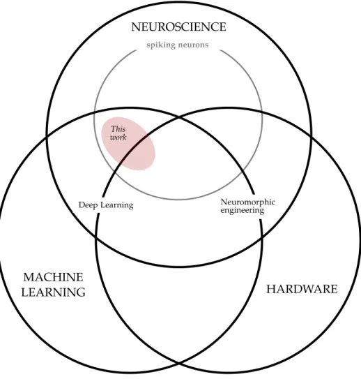
As our general paradigm, our approach will be inspired, but not bio-mimetic: while neuromorphic hardware is generally inspired by the human brain, we will only consider biological plausibility where it could prove useful from an engineering perspective. Our conceptual focus and the relationship of our research to other domains is visualized in figure 1.1.

1.3

Document structure

The remainder of this document is structured as follows:

• Chapter 2 explains general concepts and prior work that are necessary to understand the context of our research. It provides a brief overview of standard artificial neural networks and the backpropagation algorithm. It describes the basic properties of spiking neurons and how they rep-resent information. We briefly discuss the main types of neuromorphic hardware and approaches to computer simulation of spiking neural net-works. Finally, we present the state of the art of training algorithms for spiking neural networks.

• Chapter 3 presents an approach to online learning in neuromorphic sys-tems, using a biologically inspired learning rule based on spike-timing dependent plasticity. The chapter will close with a discussion of the advantages and limitations of local, biologically inspired learning rules. • Chapter 4 is concerned with the implementation of a neuromorphic ver-sion of the backpropagation algorithm. We propose SpikeGrad, a solu-tion for an on-chip implementasolu-tion of backpropagasolu-tion in spiking neural networks.

• Chapter 5 features a discussion of all results in the context of the full thesis and gives an outlook on promising future research directions.

NEUROSCIENCE

HARDWARE

spiking neurons

Deep Learning Neuromorphic_engineering

MACHINE LEARNING

This work

Figure 1.1: Schematic outline of the relationship of this thesis with other research do-mains. Deep learning can be seen as the application of some ideas from neuroscience in machine learning. Neuromorphic engineering aims to build hardware that mimics the workings of the human brain. We will focus on the utilization of artificial spik-ing neurons, a bio-inspired neuron model, for buildspik-ing deep neural networks. While this thesis has a clear focus on learning algorithm development, possible dedicated hardware implementations are taken into account in mechanism design.

Problem Statement and State of

the Art

This chapter gives a detailed overview over the main research problems that are addressed by this thesis. It contains a high level, self-contained descrip-tion of the necessary concepts in deep learning and spiking neural networks that are necessary to understand the experiments in the later chapters of the document. Additionally, it features a detailed discussion of prior research in the field of spiking neural network training.

2.1

Basic properties of deep neural networks

This section gives a brief overview of traditional deep neural networks, how they are currently used to solve machine learning problems. It introduces the notions that are necessary to understand the differences between stan-dard artificial neural networks and spiking neural network models, which are the main topic of this thesis. Additionally, it features a detailed derivation of the backpropagation algorithm that will be frequently referenced in later chapters. From now on, we refer to standard ANNs as frame-based ANNs or simply ANNs, while spiking neural networks are referred to as SNNs.

If not stated otherwise, the notation introduced in this chapter is based on a local, single neuron point of view. This allows a formulation that is more consistent with the local computation paradigm of neuromorphic hardware, which takes the single neuron and its connections as a reference point. The layer of a neuron is labeled by the index l ∈ {0, . . . , L}, where l = 0 cor-responds to the input layer and l = L to the output layer of the network. Neurons in each layer are labeled by the index i. The incoming feedforward connections of each neuron are labeled by j and the incoming top-down con-nections in the context of backpropagation by k. Which neurons are exactly referenced by these indices depends on the topology of the neural network.

2.1.1

Frame-based artificial neurons

The output (or activation) y_i of a basic artificial neuron is described by the following equation: yi =a

∑

The term in parentheses is a linear function of the inputs x_j. The parameters w_ij are called the weights. The term b_i is called bias and represents the offset of the linear function that is described by the weighted sum. The weights and biases are the main parameters of basically every artificial neural network. For a more compact representation, the bias value is sometimes represented as an element of the weights that always receives an input of 1. The activation function a is typically a non-linear function that is applied to the weighted sum.

In standard ANNs, all these variables are typically real-valued. We explain later that this stands in contrast to biological neurons, which typically output a binary spike signals. The biological justification for using real numbers as activations is based on the idea that the information propagated by the neuron is not encoded in the individual spikes, but in the firing rate of the neuron, which is real valued. However, ANNs used in machine learning have been mostly detached from biology, and real valued (floating point) numbers are simply used to represent larger variable ranges.

2.1.2

Basic layer types

We briefly summarize the properties of the most common ANN layer types, which are also used in almost all SNN implementations.

Fully connected

Fully connected (or “linear”) layers represent the simplest form of connectiv-ity. All Zoutneurons in a layer are connected to all Zinneurons of the previous

layer. Adding one bias value for each neuron, the number of parameters in a fully connected layer is therefore:

Nparams = Zin·Zout+Zout. (2.2)

Fully connected layers can be used in all layers of a neural network, but are typically found in the higher layers of a deep convolutional neural network. Convolutional

Convolutional layers are a more specialized type of neural network layer and particularly popular in image recognition. In contrast to fully connected

lay-K K Zout Xout Xin Y_in Yout Z_in

Figure 2.1: Visualization of a convolutional layer with parameters K = 3, S = 1

(without padding). The colored volume represents the weight kernel of size K2_·Zin.

The parameters K and S implicitly set the dimensions Xout and Yout based on the

dimensions Xin and Yin.

ers, they preserve spatial information in the x and y dimensions of the image. Neurons in a convolutional layer are grouped into Zout so-called feature maps

(see figure 2.1). A feature map is parameterized by a weight kernel of size K2_·Z

in, where K is the kernel dimension in x and y direction, and Zin the

number of input channels (the z dimension of the input). For the first layer, Zin is usually 3 (one dimension for each RGB channel). For higher layers, the

number of input channels Zin is the number of feature maps of the previous

layer. This weight kernel is shared by all neurons that are part of the same feature map, which is called weight sharing. Each neuron in a feature map is only connected to a sub-region of size K2 _{in the x and y dimensions of the}

input, but to the full depth Zin in the z dimension. By connecting each

neu-ron in the feature map to a different sub-region, the same kernel is applied to the full image. The output of a convolutional layer is of size Xout·Yout·Zout,

where Xout·Yout is the number of neurons in each feature map. While Zout

is chosen manually as a hyperparameter, Xout and Yout are given implicitly

by the dimension K of the kernel and the number of positions where it is applied in the input. These positions are calculated by shifting the kernel by a fixed number of pixels in the x and y directions. The number of pixels by

Xout P Zout X_in Y_in Yout P Z_in

Figure 2.2: Visualization of a pooling layer with parameters P=2, S=2. In contrast to convolutional layers, pooling layers only connect to one feature map (represented by the 3 colors) and thus reduce the input only in the x and y dimensions.

which the kernel is shifted is called the stride S of the convolutional layer. A convolutional layer is therefore fully characterized by the kernel dimension K, the stride S and the number of feature maps Zout. The number of learnable

parameters in a layer is given by the number of feature maps times the size of the kernel, plus one bias value for each feature map:

Nparams =K2·Zin·Zout+Zout. (2.3)

Often the input to a convolutional layer is artificially expanded by adding constant pixel values (typically zero) in the x and y dimensions. This process called padding is usually used to enforce certain dimensions Xout and Yout of

the convolutional layer, or to ensure that kernels size and stride fit exactly into the input dimensions Xin and Yin. For instance, a kernel size of K = 3

with a stride of 1 is typically used with padding of 1 zero valued pixel at the boundaries of the input. This way we obtain Xout =Xin and Yout =Yin.

Pooling

Convolutional layers are often combined with so-called pooling layers (see figure 2.2). Pooling layers serve to reduce the size of the input, typically in the x and y dimensions. This means that for the channel dimension of the pooling neurons we have Zout = Zin, and each pooling neuron connects only

but will be omitted here). The pooling window dimension P describes the sub-region of size P2_{to which the pooling operation is applied. Like convolutional}

layers, pooling layers have a stride parameter S. For most networks, pooling windows are non-overlapping and thus P = S. We will focus here on two types of pooling operations that are by far the most common: max pooling and average pooling. Max pooling propagates the activity of the neuron with the highest activity in the pooling window. Average pooling takes the average of all neuron activations in the pooling window.

Pooling layers are different from other neural network layers as they do not possess learnable parameters. They only perform a differentiable operation on the output of a previous convolutional layer.

2.1.3

The backpropagation algorithm

The tremendous success of modern deep learning techniques is to a large ex-tent boosted by the backpropagation algorithm (Rumelhart et al. [1986]). The backpropagation algorithm can be seen as an efficient algorithm for the op-timization of differentiable multi-layer structures. From an opop-timization per-spective, it represents an implementation of the gradient descent algorithm, which is a standard method for function optimization in machine learning. Gradient descent optimization

Let us define an artificial neural network structure as a differentiable function f with parameters (weights and biases) w, which maps an input vector X (the data) to an output vector y:

y = f(w, X) (2.4)

We now wish to find the optimal parameters w to produce a desired output of the network. For this purpose, we define a cost function_C which serves as a measure of how close we are to this objective. The optimal parameters ˆw are those that minimize the cost function over the training patterns X:

ˆ

w =arg min

w C(

y(w, X), X). (2.5)

The gradient descent training algorithm tries to solve this problem by itera-tively changing all parameters by a small amount in the negative (descending) direction of the gradient of the cost function with respect to the corresponding parameter:

∆w=₋η∂C(y(w, X), X)

or in a neuron based notation: ∆wl_ij =−η∂C(y(w, X), X) ∂wl_ij , ∆b l i =−η∂C(y(w, X), X) ∂bl_i . (2.7)

The learning rate η represents the step width by which we move in the direc-tion of descending gradient. To solve the optimizadirec-tion problem, we therefore have to find these partial derivatives for all network parameters.

The standard approach is to calculate the gradient over the full training set X (a batch). This is however computationally expensive, since the whole train-ing set has to be processed for a strain-ingle parameter update. The other extreme is to calculate the gradient over a single, random training example, and up-date the parameters for each of these examples. Due to the randomness of the samples that are drawn from the training set, this approach is called stochastic gradient descent (SGD). SGD has lower memory requirements than batch gra-dient descent and can perform more updates given the same computational resources (Bottou and LeCun [2004]).

The drawback of SGD is that it cannot exploit the massive parallelism of GPUs. The gradient is therefore usually calculated with respect to a small number of randomly drawn training examples (a mini-batch) simultaneously, which allows parallelizing the computation. The optimal size of the mini-batch depends on the GPU memory constraints, but can also be an important hyperparameter of the optimization process.

Derivation of the backpropagation algorithm

Gradient descent is a general optimization algorithm that is in principle in-dependent of the function that is optimized. As long as the function is dif-ferentiable, gradient descent can be applied to find at least a local minimum. We will now demonstrate that, in the case of an ANN, this derivative can be calculated exactly and computationally efficient. The fundamental idea is to use the chain rule from differential calculus to calculate exactly the derivative of the cost functionC with respect to each network parameter. We start in the final layer of the network, which provides the input to the cost function:

∂C ∂wL_ij = ∂C ∂y_iL ∂yL_i ∂w_ijL, ∂C ∂b_iL = ∂C ∂yL_i ∂yL_i ∂b_iL. (2.8)

The first factor in both equations depends only on the choice of the cost func-tion. The second term can be calculated based on the neuron model of the layer:

y_il =al(I_il), I_il =

∑

j

wl_ijyl−1

We call the variable I_il the integration of the neuron, which represents the total weighted input transmitted to the neuron. We can see that the output yl_i of each neuron depends on the outputs yl−1

j of the previous layer. Using the

chain rule, this gives for any layer: ∂yl_i ∂wl_ij = ∂al(I_il) ∂I_il ∂I_il ∂w_ijl =a 0_l i ylj−1, ∂yl_i ∂bl_ij =a 0_l i, (2.10)

where we have used the short notation a0l

i := ∂al(Iil)/∂Il

i. Note that this

deriva-tive is evaluated on Il

i of the forward propagation phase, which requires us to

store the Il

i or a0il for each neuron so that it is available during the

backpropa-gation phase. Substitution of (2.10) into (2.8) allows us to obtain the gradients for the top layer:

∂C ∂wL_ij = ∂C ∂y_iLa 0_L i yLj−1, ∂C ∂b_iL = ∂C ∂y_iLa 0_L i . (2.11)

As an example for a cost function that can be used, consider a cost function that consists only of the L2loss between the y_iL of the top layer and the targets

t_i:

C(yL, t) = L2(yL, t) = 1₂

∑

(yL_i −ti)2. (2.12)

This yields for the gradients (2.11): ∂_C ∂w_ijL = (y L i −ti)a0iLyLj−1, ∂_C ∂b_iL = (y L i −ti)a0iL (2.13)

We now continue by calculating the gradient for the penultimate layer L₋1: ∂C ∂wL_ij−1 =

∑

∑

A comparison of (2.15) and (2.11) shows that term ∂_C/∂yL

i was replaced by

the sum in parentheses. These two terms therefore take the same role in both equations and can be seen as an error signal. In the top layer, this error signal is directly calculated based on the cost function. In the penultimate layer, the error term is calculated based on a weighted sum that weights the errors

in the top layer by the activation function derivatives a_kL and the connecting weights wL

ki. The error in the top layer is therefore “back-propagated” through

the network. To write this more explicitly, we define the error in the top layer as:

δ_iL := ∂C ∂yL_i a

0_L

i (2.16)

and for all other layers by the recursive relation: δl_i =

∑

k

δl_k+1wl_ki+1 !

a0_il. (2.17)

Applying these definitions to equation (2.15) gives: ∂C ∂w_ijL−1 =

∑

This can be generalized to any layer of the network. (2.16) and (2.17) can thus be used to obtain the expressions of the gradients in each layer:

∂C ∂wl_ij =δ l iylj−1, ∂C ∂b_il =δ l i. (2.19)

This can now be substituted into (2.7) to obtain the update rule for all network parameters:

∆w_ijl =₋ηδ_ilyl_j−1, ∆bl_i =₋ηδ_il. (2.20) Backpropagation is thus a way to exactly solve the so-called credit assignment problem, that consists in identifying the exact contribution of a learnable net-work parameter to the output of the netnet-work. Only by identifying the con-tribution of each parameter, it is possible to globally optimize a multi-layer neural network to produce a desired output. We can see that the training of an ANN can thus be described by the set of basic equations (2.9), (2.17) and (2.20), including (2.16) for the top layer. Equations (2.9) and (2.17) describe the operations that have to be performed by each individual neuron. Since these operations are independent of other neurons in the same layer, they can be performed in parallel for all neurons of a layer. The computation that has to be performed by each neuron is in both cases a weighted sum, which is performed in hardware as a sequence of multiply-accumulate (MAC) opera-tions.

The power of backpropagation lies in the fact that it can, like the feed-forward computations in ANNs, be implemented very efficiently on modern computing hardware, in particular GPUs. This allows the optimization of the network over many iterations of a large dataset, which is crucial for the training of very deep artificial neural networks.

2.2

Spiking neurons: a bio-inspired artificial neuron

model

This remainder of this chapter motivates the use of spiking neural networks, which can be seen as an extension of ANNs that offers higher biological re-alism (Maass [1997]). We discuss major potential advantages of using this type of neuron, and a brief overview of hardware implementations of spik-ing neurons. Additionally, we discuss how spikspik-ing neurons can be simulated in computers. Finally, we present the state-of-the-art solutions for training SNNs.

2.2.1

Biological neurons

We review in this section the basic properties of biological neurons, as pre-sented in introductory neuroscience books (such as Bear et al. [2007]). The description is rather high-level and omits most of the complexity associated with biological neurons. Since our goal is to be inspired rather than bio-mimetic, we focus on those aspects of biological neurons that serve as the inspiration for the algorithms described in the later chapters of this work.

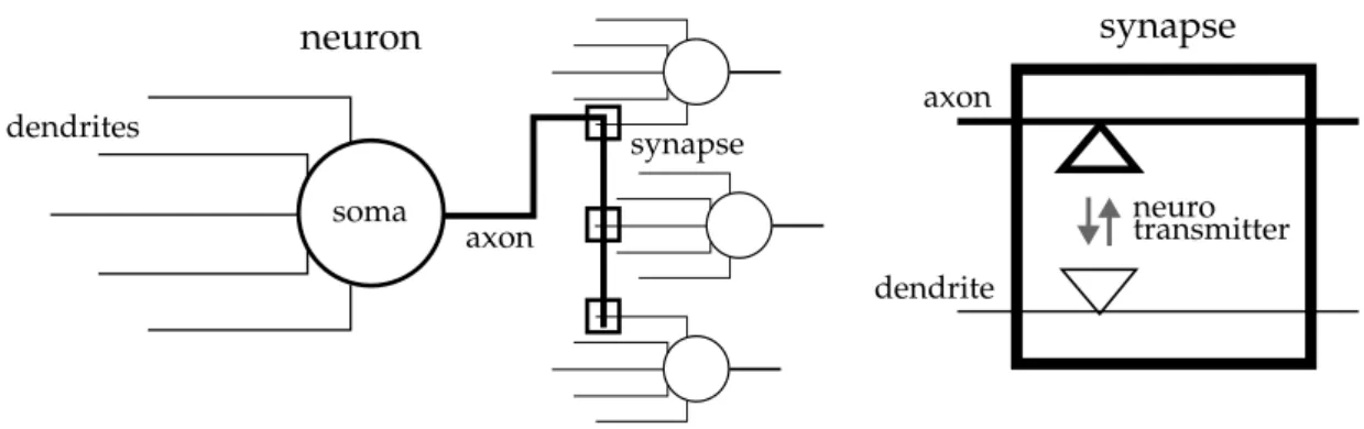
Neurons are a special type of cells that are found, among other cell types, in the human brain. They represent the cell type that is thought to be respon-sible for the execution of most cognitive tasks. On a high level of abstraction, a biological neuron consists of three fundamental parts: dendrites, soma and axon (see figure 2.3). The dendrites represent the incoming connections of a neuron that relay and process information received from other neurons. In particular, the dendrites are the part of the neuron where information is re-ceived via the synapses. Strictly speaking, a synapse does not belong to only one neuron, but represents the point of interaction between two neurons. It is the place where the axon of one neuron (the presynaptic neuron) connects to the dendrites of other neurons (the postsynaptic neurons). The axon is the single outgoing connection of a neuron, which transmits signals emitted from the neuron body. This body of the neuron, the soma, is the place where most of the typical cell organs are found. It can be imagined as the place where in-coming information from the dendrites is integrated and channeled through the axon.

Information in the neuron is stored and transmitted through electrical charge. Changes in the synapses induced by signals from other neurons will change the ion concentration in the neuron, and therefore its membrane po-tential, which is produced by a charge difference between the interior of the neuron and the surrounding environment. If the membrane potential sur-passes a certain threshold value, a rapid discharge of the neuron takes place, which resets the potential to its resting value. This discharge is propagated as a cascade via the axon of the neuron to synapses connecting to other

neu-axon dendrite neuro transmitter neuron dendrites axon soma synapse

Figure 2.3: Abstract description of a biological spiking neuron

rons. There the discharge signal will cause changes in the synapses which will trigger an exchange of chemical neurotransmitters between the two synaptic terminals. These neurotransmitters then again lead to electrical changes in the receiving neuron. Additionally, synaptic plasticity may occur, which is the change of synaptic behavior triggered by electrical and chemical interac-tion between the sending and the receiving neuron. Due to the instantaneous, event-like nature of the discharges of the neurons, which are observable as a spike in the recorded membrane potential of a neuron, these signals are often simply referred to as spikes. The important point in this description is the fact that neurons are only able to propagate binary events. How these events are processed and how information can be effectively communicated with them can depend on a large number of factors, from the synaptic behavior up to the firing dynamics of the full neural systems.

This description of biological neurons will be sufficient for most of the dis-cussions in this thesis. Neuromorphic systems using a more detailed neuron model exist (for example dendritic multi-compartment models such as used in Sacramento et al. [2018]), but will be left out here for clarity.

2.2.2

The integrate-and-fire neuron

Like traditional artificial neurons, spiking neurons can be seen as an abstract representation of biological neurons. The by far most popular mathematical model of spiking neurons is the integrate-and-fire (IF) model. IF models de-scribe the membrane potential by a variable V(t) that changes over time. To abstract from the biological inspiration for V(t) as a potential, we refer from now on to V(t) as the integration variable. This allows us to use a purely math-ematical description without having to take physical units into account. There is a large number of alternative formulations of the integrate-and-fire model, which all put an emphasis on different properties of biological neurons. We restrict ourselves in this discussion to the formulation which we consider the most common in the related literature, and the most relevant for this thesis.

In particular, we do not consider any spike transmission delays or refractory periods.

Leaky integrate-and-fire neuron

The so-called leaky integrate-and-fire (LIF) neuron has the special feature that all variables that are integrated over time are subject to leakage: they decay to zero over time, with time constants λ and λsyn. This decay serves as a kind of

high-pass filter for incoming spike trains. A basic LIF neuron can for instance be modeled by a differential equation of the form:

dV(t)

dt =−λV(t) +I(t), I(t) =

∑

neuron. The change of the integration variable is modeled by an input current I(t), which is the weighted sum of so-called synaptic traces x_j(t):

x_j(t) =

∑

ts j

e−λsyn(t−ts_j)_{. (2.22)}

In the case presented here, both synaptic traces and the integration variable are modeled as decaying variables. The traces are instantaneously increased by 1 every time a spike arrives at a time ts

j at a synapse j, and then decay

exponentially to 0. Every time the integration variable surpasses a threshold value Θ, a spike signal is emitted and V(t)is reset to its base value (typically 0). Since the trace has an explicit dependence on the time of presynaptic spike arrival, this model can take into account the exact spike timing.

The LIF model is very popular for analog hardware implementations, since the integration and decay dynamics of the neuron can easily be modeled by the behavior of sub-threshold transistors and capacitors (see section 2.2.3). Non-leaky integrate-and-fire neuron

While the LIF model is the most popular model for analog implementations, it is less popular for digital implementations, since the computation of the differential equation for every point in time can be very costly. This is es-pecially true for the exponential function that has to be calculated for each synaptic trace for every point in time. For this reason, spiking neuron models for digital implementations often use an even higher abstraction of spiking neurons, which has no leakage and is only based on accumulations:

V(t+∆t) =V(t) +

∑

j

Every input spike sj(t) will lead to an instantaneous (denoted by ∆t) increase

in the membrane potential by the value of the synaptic weight w_j. Spikes are typically modeled by a step function that is 1 when the integration variable surpasses the threshold Θ and 0 otherwise:

s(V(t)) = ( 1 if V(t)≥Θ

0 otherwise . (2.24)

After each spike, the neuron is reset to 0 or decreased by a fixed value (typi-cally Θ), which gives s(V(t))effectively a behavior similar to a delta function. Because of the absence of leakage terms, this model is often simply called IF neuron or non-leaky integrate-and-fire neuron. The attractiveness of this neuron model for digital implementations is the absence of multiplication operations if s_j(t) is the output of another IF neuron, since s(V(t)) is either one or zero. Every input spike s_j(t) will only trigger an accumulation that increments the integration variable by the weight value wj.

2.2.3

Spiking neuromorphic hardware

Neuromorphic hardware can roughly be subdivided into analog and digital approaches. A detailed review of neuromorphic engineering can be found in Schuman et al. [2017].

Analog hardware

Analog hardware uses physical processes to model certain computational functions of artificial neurons. The advantage of this approach is that op-erations that might be costly to implement as an explicit mathematical oper-ation can be realized very efficiently by the natural dynamics of the system. Additionally, real valued physical variables could in principle have almost in-finite precision. An example are the decaying potential variables or synaptic traces in the LIF neuron model, which can be modeled by the dynamics of discharging capacitors, as described in pioneering work of Mead [1990] on analog neuromorphic hardware.

Analog hardware implementations differ on the degree to which analog elements are used. Many analog implementations only perform the compu-tation in the neuron with analog elements, but keep the communication of spike signals digital. Examples of such mixed-signal neuromorphic hardware can be found for instance in Moradi et al. [2018], Qiao et al. [2015], Schmitt et al. [2017] or Neckar et al. [2019].

Major drawbacks of hardware using analog elements are high variability due to imperfections in the designed circuits (in particular when using mem-ristors), thermal noise and difficulties in memory retention. Many of these problems grow with increasing miniaturization. Another problem is that the

timescale of the physical dynamics has to be matched with the timescale of the input, which depends for example on the size of electronic elements (Chicca et al. [2014]). To the best of our knowledge, basically all neuromorphic analog implementations of spiking neurons have so far been limited to the research domain.

Digital hardware

Digital hardware represents all variables of the neuron by bits, just like a classical computer. This means that the precision of variables depends on the number of bits that is used to represent the variables. This precision also strongly influences the energy consumption of the basic operations and the memory requirements for variable storage.

The great advantage of digital designs compared to analog hardware is that the precision of variables is controllable and guaranteed. Additionally, digital hardware can be designed with established state-of-the-art techniques for chip design and manufacturing.

A large number of digital designs exists for spiking neuromorphic hard-ware. Examples of industry designs of Application Specific Integrated Cir-cuits (ASICs) include Davies et al. [2018] and Merolla et al. [2014], while Frenkel et al. [2018] and Lorrain [2018] represent academic research chips. Even the industrial designs have however not yet been integrated into many commercial products. Alternatively, due to the high production costs of ASICs, other research groups have focused on implementing SNNs in Field Programmable Gate Arrays (FPGAs) (for instance Yousefzadeh et al. [2017])

One drawback of digital designs is that they are suitable for the implemen-tation of spiking neurons only to a limited extent. Classical high performance computing hardware, such as GPUs, is highly vectorized and heavily exploits parallelism in data processing. This kind of processing is very suitable for the operations that have to be performed in standard artificial neural net-works. Spiking neural networks operate however in a strongly asynchronous fashion, with high spatial and temporal sparsity. An efficient implementation of a spiking neural network therefore requires a design that differs strongly from most existing high performance computing hardware. Typically, digital neuromorphic hardware uses the so-called address-event representation (AER) protocol, where values are communicated by events that consist of an address and a timestamp.

A particular problem when implementing the IF neuron in digital hard-ware is the large number of memory accesses that are necessary to update the integration variable with each incoming spike. In particular if the memory is not located in direct vicinity of the processing element that performs the op-erations, the high number of memory transfers can impact the energy budget more strongly that the computing operation itself (Horowitz [2014]).

In this thesis, we chose to design most algorithms with a digital imple-mentation in mind. The main reason for this are the high precision require-ments currently imposed by most applications that use deep learning solu-tions. Additionally, computation in digital hardware can be exactly modeled by computer simulation. Designing algorithms for analog circuits would re-quire us to make a large number of assumptions on the potential hardware and its physical properties. Additionally, all state-of-the-art standard deep neural network solutions are implemented in digital hardware. It is therefore easier to compare a spiking network with a standard ANN in a simulated digital framework, since this does not necessarily require an actual dedicated hardware implementation.

2.2.4

Information encoding in spiking networks

This section briefly reviews the different approaches to encode information in spiking neural networks. We show that the optimal coding strategy is deeply connected to the choice of the neuron model, the hardware constraints and the application target.

Rate coding

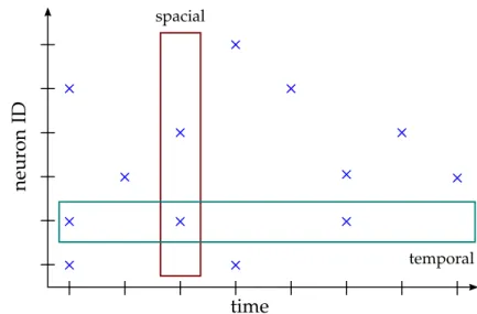
The probably most common and best studied approach to encode information in SNNs is to use the firing rate. This rate can be either defined with respect to a certain explicit physical time (e.g. events per second), as it is usually done in neuroscience, or with respect to an implicit time (e.g. per stimulus or per example). The basic idea is to represent information in an accumulated quan-tity that has the same value irrespective of the exact time of spike arrival. This implies that the information representation capacity of the spiking neuron in-creases with the number of spikes it is able to emit in a certain time. Figure 2.4 demonstrates the principle of rate coding for different measurement inter-val sizes. It can be seen that depending on how long the observation window is, the measured firing rates can deviate quite strongly from each other. If the neuron should be able to represent the same number independent of the ob-servation time, the firing should be as regular as possible. In a counting-based representation, where the observation window always has the same size, the timing of spikes is irrelevant and only the total number of spikes is required to represent a number.

In particular in digital implementations, the efficiency of rate coding de-pends on the cost of the operation induced by a single spike. If the cost of such an operation is rather high, a spiking network can be less efficient than its frame-based counterpart, since many spikes may be necessary to commu-nicate the same information. For instance, we require n spike events to enable a neuron to represent integer numbers in the range[0, n]. To represent all