is an open access repository that collects the work of Arts et Métiers Institute of
Technology researchers and makes it freely available over the web where possible.
This is an author-deposited version published in: https://sam.ensam.eu
Handle ID: .http://hdl.handle.net/10985/9862
To cite this version :
Thomas HENNERON, Stéphane CLENET - Proper Generalized Decomposition method applied to solve 3D Magneto Quasistatic Field Problems coupling with External Electric Circuits - IEEE transactions on Magnetics - Vol. 51, n°6, p.1-10 - 2014
Any correspondence concerning this service should be sent to the repository
Proper Generalized Decomposition method applied to solve 3D
Magneto Quasistatic Field Problems coupling with External Electric
Circuits
T. Henneron
1, S. Clénet
21L2EP, Université Lille 1, 59655 Villeneuve d’Ascq, France. 2
L2EP, Arts et Métiers ParisTech, 59046 Lille, France.
In the domain of numerical computation, Proper Generalized Decomposition (PGD), which consists of approximating the solution by a truncated sum of separable functions, is more and more applied in mechanics and has shown its efficiency in terms of computation time and memory requirements. We propose to evaluate the PGD method in order to solve 3D quasi static field problems coupling with an external electric circuit. The numerical model, obtained from the PGD formulation, is used to study 3D examples. The results are compared to those obtained when solving the full original problem. It is shown in this paper that the computation time rate versus the number of time steps is very small compared to the one a classical time stepping method and can be very efficient to solve problems when small time steps are required.
Index Terms— Finite element method, quasi static problem, electric circuit, reduced order model, proper generalized decomposition
I. INTRODUCTION
n quasistatic field problems, the magnetic and electric fields are time and space dependent. To calculate these fields, Maxwell’s equations are discretised in the space and time domains. The finite element method is often used to approximate the fields in the space domain. In the time domain, a time stepping scheme is often used. In the case of a fine space mesh and a small time step, the computation time of this model, the so-called full model in what follows, is sometimes prohibitive. To circumvent this issue, model order reduction methods are proposed in the literature. These approaches consist of seeking a solution in a subspace of the approximation space of the full model. Several approaches have been developed. We can distinguish priori and
a-posteriori methods.
With the a-posteriori approaches, the solution of the reduced model is sought in a subspace of the approximation space of the full problem. The projection operator between these two spaces is determined from “well chosen” solutions of the full model. The Proper Orthogonal Decomposition or Lanczos-Arnoldi approaches can be used to determine the discrete projection operator [1-4]. Applying the projection operator to the full model, a model of reduced size is constructed which can be solved very quickly. An approximated solution of the full model can be reconstructed by projecting the solution of the reduced model in the approximation space of the full model. In electromagnetics modeling, the a-posteriori approaches have been successfully applied to solve static and quasistatic problems [5-9].
With the a-priori method, the subspace of approximation is not known a-priori and it is constructed using an iterative procedure. The solution is assumed to be written as a sum of separable functions. In this context, Proper Generalized Decomposition (PGD) has been developed since the early 2000s in computational mechanics [10-11]. The PGD approach can be applied to solve systems of partial differential
equations in the time domain. The solution is approximated by a sum of M separable functions Si(t)Ri(x) in time and space. Each separable function Si(t)Ri(x) is so-called mode. The function Si(t) satisfies an ordinary differential equation which can be solved numerically using a time-stepping method. The function Ri(x) is the solution of a stationary partial derivative equation which can be solved using the finite element method. Each mode i is determined by an iterative process and depends on the previous modes. In computational electromagnetics, the PGD method has been applied to study a fuel cell polymeric membrane model [12]. In static electromagnetism, the behavior of a Soft Magnetic Composite Material has been modelled [13]. In magneto-quasistatics, the skin effect in a rectangular slot using a 1D model has been developed in [14]. The PGD has been also compared in [15] to the POD approach on a quasistatic example. It has been shown that the POD method is more efficient in terms of computation time to solve quasistatic problems supplied by low frequency content sources. It has been shown also that the computation time with the PGD is almost independent of the number of time steps. The behavior of the two methods of reduction at high frequency, when the required number of time steps is large, hasn’t been investigated yet. Moreover, in all the previous examples, the coupling with the external circuit, which is a key point to treat real applications, has not been addressed.
In this paper, we propose to study a 3D magneto-quasistatic field problem coupling with an external electric circuit using the PGD approach. We propose to evaluate the performances of the PGD model accounting for a circuit coupling. For a given device, the time step depends highly on the voltage supply. To study the influence of the time step on the computation time, two cases are investigated. In the first case, the voltage supply has a narrow frequency range. In the second case, the harmonic content of the voltage supply is rich on a wide frequency range which requires the use of very small time step. The last case is often met in practice when the voltage source is a high frequency power converter. First, the
quasistatic field problem and the coupling with the electric circuit are introduced. Then, the application of the PGD to solve the quasistatic problem is explained. Finally, a comparison with the solution obtained from the standard approach, fully discretised in the time and space domains, is presented.
II. MAGNETO-QUASISTATIC PROBLEM
A. Problem Description
Let us consider a domain D with a boundary Γ (Γ=ΓB∪ΓH and ΓB∩ΓH=0) and a conducting domain Dc, included in D, of boundary Γc with Γc=ΓJind∪ΓE and ΓJind∩ΓE=0 (Fig. 1). For sake of clarity, we will assume that the domain D contains only one stranded inductor, even though the approach remains valid with several stranded inductors.
N(x)i(t) ΓB ΓH ΓE(ΓB) ΓJind D Dc ΓB R v(t)
Fig.1. Computational domain
In quasistatics, Maxwell’s equations can be written under the form:
curl E(x,t) = -∂tB(x,t)
curl H(x,t) = Jind(x,t) + N(x)i(t) div B(x,t) = 0
div (Jind (x,t) + N(x)i(t)) =0
(1.a) (1.b) (2.a) (2.b) with B the magnetic flux density, H the magnetic field, E the electric field, Jind the eddy current density defined only in the conducting domain Dc, N and i the unit current density vector and the current flowing through the stranded inductor. The electric and magnetic behaviour laws are:
B(x,t) = µ0µr H(x,t) in D Jind (x,t) = σ E(x,t) in Dc
(3.a) (3.b)
with µ0 the magnetic permeability of the vacuum, µr the relative permeability of the material, σ the electric conductivity. The boundary conditions are given by:
B(x,t)⋅⋅⋅⋅n=0 on ΓB and H(x,t)×n=0 on ΓH Jind(x,t)⋅⋅⋅⋅n=0 on ΓJind and E(x,t)×n=0 on ΓE
(4) (5) with n the outward unit normal vector. A gauge condition needs to be added to impose the uniqueness of the solution in
non conductive region (σ=0). To solve the problem discretised using the Finite Element Method, an iterative solver is used providing an implicit gauge [16].
In order to impose the voltage v at the terminals of the stranded inductor, the following relation must also be taken into account, v(t) Ri(t) dt (t) d = + Φ (6)
with R the resistance and Φ the magnetic flux linkage associated with the stranded inductor. We aim to determine a solution to the previous problem on D×[0,T] with T the length of the maximum time.
B. A* formulation
To solve the previous problem, the A* formulation can be used. A modified magnetic vector potential A*(x,t) is defined in the whole domain from (1-a) and (2-a),
B(x,t) = curl A*(x,t) and E(x,t) = -∂tA*(x,t)
with A*(x,t)×n=0 on ΓB and ΓE.
(7)
We define L2([0,T]) and L2([0,T]) the spaces of square integrable scalar and vectorial functions on [0,T] and L2(D) the space of square integrable vectorial functions on D [17]. The vector potential A* belongs to the space H(grad,[0,T];H(curl,D)) defined such that H(grad,[0,T]) = {u∈L2([0,T]); grad u∈L2([0,T])} and H(curl,D)= {u∈L2(D); curl u∈L2(D)}. The current i belongs to the space L2([0,T]). To determine a solution to the problem on D×[0,T], weak forms of (1.b) and (6) can be used in combination with (3) and (7): 0 t)dtdD , ( ' ) ( i(t) t)dtdD , ( ' t) , ( σ t) , ( ' t) , ( µ 1 D T 0 t D T 0 = ⋅ − ⋅ ∂ + ⋅
∫ ∫
∫ ∫
x A x N x A x A x A curl x A curl * * (8)∫
∫
Φ ⋅ + ⋅ = ⋅ T 0 T 0 (t)dt i' v(t) (t)dt i' Ri(t) (t) i' dt (t) d (9)with A’ and i’ test functions belongs to the same functional spaces as A* and i respectively.
Equations (8) and (9) are related by the expression of the magnetic flux linkage as a function of A*,
∫
⋅ = D )dD ( t) , ( Φ(t) A x N x * (10)III. PROPER GENERALIZED DECOMPOSITION
A. Separated representation
In order to solve equations (8) and (9), a method based on the PGD approach can be used [10, 11, 15]. The magnetic vector potential is thus approximated by a separated representation of space and time functions, as in
Manuscript received January 1, 2008 (date on which paper was submitted for review). Corresponding author: T. Henneron (e-mail: [email protected]).
∑
= ≈ M 1 n n n( )S (t) t) , (x R x A * (11)with x∈D, t∈[0,T] and M the number of terms of the expansion. The aim is to find a separated representation of A* with M functions. The functions Rn(x) and Sn(t) belong to the space H(curl,D) and H(grad,[0,T]) respectively. The test function A' in the weak form (8) associated with the nth mode can be written such that:
(t)' )S ( (t) S )' ( t) , ( ' x Rn x n Rn x n A = + (12)
with Rn(x)' and Sn(t)' the test functions defined in the same spaces of Rn(x) and Sn(t) respectively. The current is also decomposed into a sum of currents:
∑
= ≈ M 1 n n(t) i i(t) (13)To compute the functions Rn(x), Sn(t) and in(t), an iterative enrichment method is used. The triplet (Rn(x), Sn(t), in(t)), also called a mode, is calculated with respect to the previous triplets (Ri(x), Si(t) , ii(t)) with i∈[1,n-1]. The number of modes in (11) and (13) is not known a-priori by the user, it can be determined by assuming that the influence of the functions Rn(x), Sn(t)and in(t)decreases as a function of n, the modes are added to the approximated solutions (11) and (13) until the components of the mode n, the current in(t) on [0,T] and Rn(x)Sn(t) on D×[0,T] satisfy the following condition:
and ε (t)
in 2[0;T]≤ n Rn(x)Sn(t)2(D×[0;T])≤εn (14)
with a criterion εn fixed by the user.
B. Computation of (Rn(x), Sn(t), in(t))
We assume that we have already calculated the triplets (Ri(x), Si(t), ii(t)) with i∈[1,n-1]. To calculate the triplet (Rn(x), Sn(t), in(t)), two sets of equation, that will be determined in the following from (8) and (9), are solved iteratively. First, we suppose that Rn(x) is known. Then, the function Rn(x)' vanishes in (12) and the test function A' is equal to Rn(x)Sn(t)'. Equations (8) and (9) are solved in order to determine the functions Sn(t) and in(t). Replacing in (8) and (9) A' by Rn(x)Sn(t)' and A* by its expansion (11) truncated up to the mode n, we obtain the two following equations,
∑ ∫
∫
∑ ∫
∫
∑ ∫
∫
∫
∫
∫
∫
∫
∫
− = − = − = ⋅ ⋅ + ⋅ ⋅ − ⋅ ⋅ − = ⋅ ⋅ − ⋅ ⋅ + ⋅ ⋅ 1 n 1 i D T 0 n i n 1 n 1 i D T 0 n i n i 1 n 1 i D T 0 n i n i D T 0 n n n D T 0 n n n n D T 0 n n n n dt ' (t) S (t) i )dD ( ) ( dt ' (t) S dt (t) dS )dD ( ) ( dt ' (t) S (t) S )dD ( ) ( µ 1 dt ' (t) S (t) i )dD ( ) ( dt ' (t) S dt (t) dS )dD ( ) ( dt ' (t) S (t) S )dD ( ) ( µ 1 x R x N x R x R x R curl x R curl x R x N x R x R x R curl x R curl σ σ (15.a)∑
∑ ∫
∫
∫
∫
∫
∫
− = − = − ⋅ ⋅ − ⋅ = ⋅ + ⋅ ⋅ 1 n 1 i i 1 n 1 i D T 0 n i i T 0 n T 0 n n D T 0 n n n (t) Ri dt ' (t) i dt (t) dS )dD ( ) ( dt (t)' i v(t) (t)' i (t) i R dt ' (t) i dt (t) dS )dD ( ) ( x N x R x N x R (15.b)We can see that we have taken advantage of the separable form of the expression of the vector potential A* to obtain two equations with terms written as a product of an integral on the space and an integral on the time interval. This aspect is the key point of the PGD approach. We can note that (15) are weak forms of the following Ordinary Differential Equation (ODE) systems (where S'n(t) and i'n(t) are the test functions and Sn(t) and in(t) the unknowns):
(t) F (t) i C dt (t) dS B (t) S AR n + R n − Rn = R (t) F dt (t) dS C (t) Ri i n R n + = with , )dD ( ) ( (t) i )dD ( ) ( dt (t) dS )dD ( ) ( µ 1 (t) S (t) F , )dD ( ) ( C , )dD ( ) ( B , )dD ( ) ( µ 1 A 1 n 1 i D n i 1 n 1 i D n i i 1 n 1 i D n i i R D n R D n n R D n n R
∑
∫
∑
∫
∑
∫
∫
∫
∫
− = − = − = ⋅ + ⋅ − ⋅ − = ⋅ = ⋅ = ⋅ = x R x N x R x R x R curl x R curl x R x N x R x R x R curl x R curl σ σ∑
∑ ∫
− = − = − ⋅ − = n1 1 k k 1 n 1 k k D k i Ri (t) dt (t) dS )dD ( ) ( v(t) (t) F R x Nx (16.a) (16.b)Secondly, to calculate the function Rn(x), we assume that the functions Sn(t) and in(t) are known. In this case, the function Sn(t)' vanishes in (12) and the test function A' is equal to
Rn(x)'Sn(t). Replacing in (8), A' by Rn(x)'Sn(t) and A* by its expansion (11) truncated up to the mode n, we obtain
∑
∫
∫
∑
∫
∫
∑
∫
∫
∫
∫
∫
∫
∫
∫
− = − = − = ⋅ ⋅ + ⋅ ⋅ − ⋅ ⋅ − ⋅ ⋅ = ⋅ ⋅ + ⋅ ⋅ 1 n 1 i D n T 0 n i 1 n 1 i D n i T 0 n i 1 n 1 i D n i T 0 n i D n T 0 n n D n n T 0 n n D n n T 0 n n dD )' ( ) ( dt (t) S (t) i dD )' ( ) ( dt (t) S dt (t) dS dD )' ( ) ( µ 1 (t)dt S (t) S dD )' ( ) ( dt (t) S (t) i dD )' ( ) ( dt (t) S dt (t) dS dD )' ( ) ( µ 1 dt (t) S (t) S x R x N x R x R x R curl x R curl x R x N x R x R x R curl x R curl σ σ (17)Like in (15), we have taken advantage of the separable form of A*. The equation is also the weak form of a Partial Differential Equation (PDE) where Rn(x) is the unknown and Rn' (x) is the test function that can be written as
) ( ) ( σ B )) ( µ 1 ( AScurl curlRn x + S Rn x =FS x with
∑
∫
∑
∫
∑
∫
∫
∫
∫
− = − = − = ⋅ + ⋅ − ⋅ − ⋅ = ⋅ = ⋅ = 1 n 1 i T 0 n i 1 n 1 i T 0 n i i 1 n 1 i T 0 n i i T 0 n S T 0 n n S T 0 n n S dt (t) S (t) i ) ( dt (t) S dt (t) dS ) ( R (t)dt S (t) S )) ( µ 1 dt (t) S i(t) ) ( ) ( , dt (t) S dt (t) dS B , dt (t) S (t) S A x N x x R curl curl( x N x F σ (18)The triplet (Rn(x), Sn(t), in(t)) must satisfy (16) and (18) according that the previous triplets (Ri(x), Si(t), ii(t)) with i∈[1,n-1] are known. An iterative procedure based on a fixed point approach is used. We denote (Rnj-1(x), Snj-1(t), inj-1(t)) the solution obtained at the jth-1 iteration. At the jth iteration, the PDE (18) is solved to obtain the function Rnj(x) using the previous functions Snj-1(t) and inj-1(t) to determine the coefficients As and Bs and the function Fs(x). The PDE (18) is solved applying the Finite Element Method but any other numerical method can be applied. Then, from the solution Rnj(x), the coefficients AR, BR and CR and the functions FR(t) and Fi(t) are calculated (see (16)). Then, the ODE (16) is solved using an implicit Euler scheme in order to obtain the functions Snj(t) and inj(t). The triplets (Rnj(x), Snj(t), inj(t)) and (Rnj-1(x), Snj-1(t), inj-1(t)) are then compared. The error between the triplets of functions can be determined by:
fp 2 j 2 1 -j j ε Y Y Y ≤ − (19)
with Y the components of the functions Rn(x), Sn(t) or in(t) and εfp a criterion fixed by the user. If the error between the two triplets is too high, the process is repeated. At the first iteration of this procedure, the functions Sn0(t) and in0(t) are initialized at Sn-1(t) and in-1(t) respectively.
The proof of convergence for separated solution representation methods has been given in [18]. Our developed approach does not belong to this class of problems. However, even though the proof is not given, our problem is similar to other ones which have been solved with the PGD approach and for which no convergence proof has been given yet [19]. A lot of problems in engineering have been solved with the help of the PGD method showing in practise its efficiency but also its limits.
C. Complexity analysis
The complexity of the PGD model is compared to this one of the full model solved using a classical time stepping method. We note nu the number of unknowns in the space domain and nt the number of time steps. The complexity of the full model is given by O(ntnu
α
) with 1≤α≤2 depending on the method used to solve the linear equation system. The complexity varies linearly with nt.
For the PGD model, the number of unknowns associated with the functions Rn(x) and Sn(t) are nu and nt respectively. The number of unknowns of the functions in(t) is the same as the function Sn(t). Then, the complexity of the PGD model can be given by O(M kfp(2nt+nu
α
)) with M the number of modes and kfp the maximum iteration number of the loop used to determine a mode of rank n (Section III-B). The variation with the time step number remains linear however the term 2nt is generally negligible versus the term nuα since the unknown number in the space domain nu are generally higher than the number of time steps nt. Consequently, the complexity of the PGD models can be approximated by O(M kfp nu
α ) and depends only on the number of unknowns in the space domain, even for small time steps.
IV. ACADEMIC EXAMPLE
Two conducting plates submitted to a magnetic field created by a stranded inductor are considered. Due to its symmetry, only one eighth of the problem is modeled (Fig. 2). The number of turns of the inductor is equal to 100 and its resistance 0.75Ω. The relative magnetic permeability of the conducting plate is fixed at 1 and its electric conductivity at 1MS/m. The 3D spatial mesh has 14970 nodes and 80199 tetrahedra. Two types of supply voltage are considered. In the first case, a periodic square voltage is imposed. In the second case, a Pulse-Width Modulation (PWM) voltage is fixed. The problem has been solved using the modified vector potential A* formulation. The PGD method presented in the previous section has been applied to obtain an approximated solution. In order to evaluate the efficiency of the PGD method, the same problem has been solved with a classic EF model using an implicit Euler scheme. The results obtained from this numerical model will be considered as the reference results.
stranded inductor
conducting plate
SB
SJ
Fig.2. Structure of the studied problem
A. Supply by a periodic square voltage
The inductor is supplied by a periodic square voltage at a frequency equal to 10kHz. The magnitude is fixed at 1V during the half period and at 0V during the other half of the period. The time interval of simulation is fixed at [0;875µs] with a time step of 2.5µs.
1) Global quantities versus the number of modes
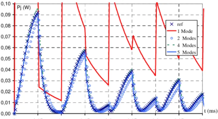
The global quantities obtained from the PGD method are compared with those computed from the full model. We assume that the full model gives results sufficiently accurate to be considered as a reference. Figures 3 and 4 present the evolution of the current and of the Joule losses obtained from the PGD method on the interval [0,T] for a different number of modes. We can see that at least 4 modes are required to obtain a current evolution close to the one given by the full model. With the Joule losses, we can see in Fig.4 that at least 5 modes are required and that the first mode gives very different results from the reference model. To illustrate this point, we present in Fig.5 the evolution of the relative errors εi and εPj for the current and Joule losses as a function of the number of modes. The error is expressed such that:
2 ref 2 PGD ref Y Y Y Y ε = − (20)
with Yref and YPGD the evolutions of the quantity of interest Y obtained from the full model Yref and the reduced model YPGD. We can show that the current converges up to the reference with a lower number of modes than the Joules losses. To have an error close to 0.1%, 6 modes are necessary to correctly express the solution using the expression (11) for the current and 8 modes for the Joules losses.
0,00 0,10 0,20 0,30 0,40 0,50 0,60 0,70 0,80 0,90 1,00 0 0,05 0,1 0,15 0,2 0,25 0,3 0,35 0,4 t (ms) i (A) ref 1 Mode 2 Modes 4 Modes
Fig.3. Evolution of the current as a function of the number of modes
0,00 0,01 0,02 0,03 0,04 0,05 0,06 0,07 0,08 0,09 0,10 0 0,05 0,1 0,15 0,2 0,25 0,3 0,35 0,4 t (ms) Pj (W) ref 1 Mode 2 Modes 4 Modes 5 Modes
Fig.4. Evolution of the Joule losses as a function of the number of modes
0 0,5 1 1,5 2 2,5 3 3,5 4 4,5 5 0 2 4 6 8 10 12 number of modes % ei ePj
Fig.5. Error of the current and the Joule losses as a function of the number of modes
In order to evaluate the contribution of each mode to the current shape, Fig. 6 presents the evolution of the first four modes. We can observe that the contribution of the current in(t) decreases when the rank of the mode n increases. The current i1(t) gives an estimation of the mean value of the current but we can see strong discontinuities on the current that are not physical. The current modes in(t) with n>1 contribute to reducing these discontinuities of i(t).
-0,2 0 0,2 0,4 0,6 0,8 1 0 0,05 0,1 0,15 0,2 0,25 0,3 0,35 t (ms)0,4 (A) i1(t) i2(t) i3(t) i4(t) i(t)
Fig.6. Current evolutions for the first four modes
In a similar way, it is possible to study the influence of the functions Sn(t) related to the vector potential A* (see (11)). Figure 7 gives the evolutions of these functions for the first four modes. We can observe a transient state for all the functions Sn(t). The influence of S1(t) is the most significant. We can see also that the contribution of Sn(t) with n>1
decreases rapidly. The assumption of a decreasing contribution of the mode with their rank is verified on the example studied. -0,1 0 0,1 0,2 0,3 0,4 0,5 0,6 0,7 0,8 0 0,05 0,1 0,15 0,2 0,25 0,3 0,35 0,4 t (ms) S1(t) S2(t) S3(t) S4(t)
Fig.7. Evolution of the functions Sn(t) for the four first modes
2) Local quantities versus the number of modes
From expression (11) of the solution, it is possible to present a distribution of the magnetic flux density associated with each mode. Figures 8 and 9 present the distributions of Bi(x,tj)=curl Ri(x)Si(tj) with i=1,2 at a given time tj in a cross section SB of the structure presented in Fig. 2. The distribution of B1 appears to be close to the one obtained from a magnetostatic problem when the stranded inductor is supplied and the conductivity in the plate is equal to zero. The distribution of B2 is like a reaction magnetic flux density created by the eddy current density in the conducting plate. In the same way, the distribution of the eddy current density can be presented for each mode at a given time step. Figures 10 and 11 present the distributions of J1 and J2 in the cross sections SJ of the conducting plate presented in Fig. 2. We can observe that the directions of these fields are opposite, with J1 having the same direction as N(x)i(tj) flowing through the stranded inductor. The distribution of J2 is in the opposite direction, creating the reaction magnetic field B2 (Fig. 9).
Fig.8. Distribution of B1(T)
Fig.9. Distribution of B2(T)
Fig.10. Distribution of J1(A/m2)
Fig.11. Distribution of J2(A/m2)
In terms of the distribution of the fields, Figures 12 and 13 (resp. 14 and 15) present the distribution of B (resp. J) on SB (resp. SJ) obtained from a number of modes equal to 8 and 15 respectively. With 8 modes, we can observe that we obtain a non-physical distribution of the magnetic flux density. The distribution has sufficient accuracy with 15 modes. For the eddy current density in the conducting plate, the distributions of J are close. In order to compare the distributions of the field obtained from the reduced model and the reference problem, Fig. 16 and 17 present the distribution of the difference of the magnetic flux density obtained from the full model and the reduced model with 8 and 15 modes. For both cases, the maximum of the error is not located where the magnetic flux density is the most important but in the conducting plate. The maximum values of the error distribution decrease when the
number of modes is increasing. The maximum error has been reduced by a factor of 2.5 by adding 7 modes to the approximated solution.
Non physical distribution
Fig.12. Distribution of B(T) for 8 modes
Fig.13. Distribution of B(T) for 15 modes
Fig.14. Distribution of J(T) for 8 modes
Fig.15. Distribution of J(T) for 15 modes
Fig.16. Difference between Bref and BPGD with 8 modes
Fig.17. Difference between Bref and BPGD with 15 modes
3) Computation time
The computation time for the full model is 35min. The reduced model with 8 modes requires 4min30s. In this case, the error given by (20) with respect to the evolution of the Joule losses is close to 0.1%. To study the global quantities of the problem, this number of mode is sufficient. If we are interested by the local value of the magnetic flux density, we have shown that, in this case, at least 15 modes are required. With 15 modes to approximate the solution, we obtain an error inferior to 0.01% with respect to the evolution of the Joule losses and a distribution of B close to that of the reference model. In this case, the computation time is 8min, which is nonetheless quicker than the reference model.
B. Supply by a PWM voltage
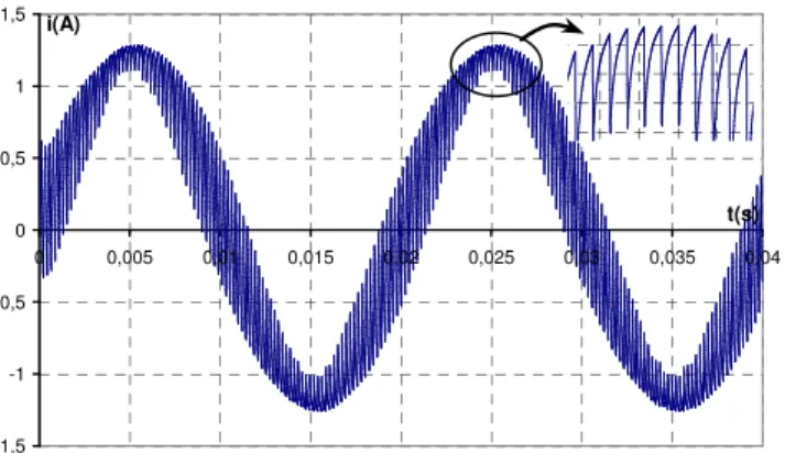
Figure 18 presents a description of the supply of the stranded inductor. This is supplied by a 2-level PWM voltage source, and the carrier frequency is equal to 50Hz. The quantity of interest is the current. According to the previous study, the number of modes to approximate the solution has been fixed at 8. Two switching frequencies are considered (f1 = 500Hz and f2 = 5KHz) in order to verify the accuracy of the PGD model. The time interval of simulation is fixed at [0;0.04s] corresponding to two periods of the carrier frequency. To account for the switching of the converter switches, the time step should be at least fifty times lower than the switching frequency. The time steps are equal to 40µs for f1 and to 4µs for f2. In this application, the number of time steps is much higher than in the previous application. Figures 19 and 20 present the evolutions of the current obtained from the two switching frequencies. The wave shapes of the current are correct for both switching frequencies. For the case with the switching frequency f2, we can observe a transient state at the beginning of the simulation due to the high frequency. For the switching frequencies f1 and f2, the number of time steps is 1000 and 10000 respectively, and the computation times are 5min30s and 10min40s respectively. We can see that even though we have increased the number of time steps by 10, the computation time has been multiplied by only a factor of 2. Moreover, the computation time is of the same order than the one in the previous application which was 4min30s for a smaller number of time steps. It confirms the complexity analysis presented in the section III-D where it is shown that the time calculation doesn’t depend for a given number of modes on the time step (if the time step number is small compared to the number of unknowns of the mesh). The PGD approach shows in that example its powerfulness when it comes to treating problem with very small time steps.
U
R
L
FE model
Fig.18. Evolution of the current with the switching frequency f1
-1,5 -1 -0,5 0 0,5 1 1,5 0 0,005 0,01 0,015 0,02 0,025 0,03 0,035 0,04 t(s) i(A)
Fig.19. Evolution of the current with the switching frequency f1
-1,5 -1 -0,5 0 0,5 1 1,5 0 0,005 0,01 0,015 0,02 0,025 0,03 0,035 0,04 t(s) i(A)
Fig.20. Evolution of the current with the switching frequency f2
V. INDUSTRIAL APPLICATION
In order to evaluate the efficiently of the PGD approach on a realistic application, a squirrel cage induction machine is considered (Fig. 21) [20]. The aim is to study the evolution of the global quantities versus the time when the machine is supplied at standstill. The spatial mesh has 93300 nodes and 93154 prismatic elements in one layer along the machine axis. Like the previous example, two types of supply voltage are considered. The machine is supplied first by sinusoidal voltages and then by a Pulse-Width Modulation (PWM) voltage source inverter. Three external circuit equations (see (9)) corresponding to the three phases are considered. In order to limit the number of modes, after each enrichment step, the set of the functions Sn(t) and the currents are recalculated according to the method presented in [11]. The reference is the solution of the full problem solved with a classical finite element model using an implicit Euler scheme.
phase 1 phase 2 phase 3 rotor bar
Fig.21. Structure of the squirrel cage induction machine
A. Supply by sinusoidal voltages
The three phases of the stator are supplied by sinusoidal voltages at a frequency equal to 50Hz. The time interval of simulation is fixed at [0;100ms] with a time step of 0.5ms. The evolution of the relative errors for the magnetic energy and Joule losses in the rotor bars as a function of the number of modes are presented in Fig. 22. We can show that the magnetic energy converges towards the reference with a lower number of modes than the Joule losses in the rotor bars. With 15 modes, the error is lower than 0.2% for the Joule losses and to 0.001% for the magnetic energy. Figure 23 presents the evolution of the currents obtained from the full model and from the PGD model with 15 modes. The computation times
are 17 min and 3min for the full and PGD models respectively. 0 10 20 30 40 50 60 70 80 90 100 0 2 4 6 8 10 12 14 (%) ePJ eEmag
Fig.22. Error of the magnetic energy (eEmag) and the Joule losses (ePJ) as a function of the number of modes with sinusoidal voltages
-2500 -2000 -1500 -1000 -500 0 500 1000 1500 2000 2500 0 0,005 0,01 0,015 0,02 0,025 0,03 0,035 0,04 0,045 0,05 t(s)
(A) i1(t) ref i2(t) ref i3(t) ref
i1(t) pgd i2(t) pgd i3(t) pgd
Fig.23. Evolution of the currents with sinusoidal voltages
(max. relative error = 4.9%)
B. Supply by PWM voltages
The three phases of the stator are supplied by 2-level PWM voltages, and the carrier frequency is equal to 50Hz. The switching frequency is 1kHz. The time interval of simulation is fixed at [0;40ms] with a time step of 50µs. The evolution of the relative errors for the magnetic energy and Joule losses as a function of the number of modes are presented in Fig. 24. Due to the complex shape of the PWM voltages, the number of modes is higher than in the case of a sinusoidal supply to obtain a good agreement of the global values with the full model. Like in the previous case, the magnetic energy converges up to the reference with a lower number of modes than the Joule losses in the rotor bars. With 30 modes, the error is close to 0.4% for the Joule losses and to 0.002% for the magnetic energy. Figures 25 and 26 present the evolution of the currents and of the Joule losses obtained from the full model and from the PGD model with 30 modes. The evolutions of the quantities of interest obtained from the PGD model are close to those from the reference model. The computation times are 55min and 8min for the full and PGD models respectively. With the PWM supply, twice more modes are required with the PGD to obtain a solution close to the reference one. Indeed, the current wave shape is less smooth than in the case of a sinusoidal supply.We can notice that the speed up is not so significant as it was in the previous example when decreasing the time step. However, we can see that the PGD on this example enables to reduce the
computation time compared to a time stepping method.
0 10 20 30 40 50 60 70 80 90 100 0 5 10 15 20 25 30 (%) ePj eEmag
Fig.24. Error of the magnetic energy (eEmag) and the Joule losses (ePJ) as a function of the number of modes with PWM voltages
-2500 -2000 -1500 -1000 -500 0 500 1000 1500 2000 2500 0 0,002 0,004 0,006 0,008 0,01 0,012 0,014 0,016 0,018t(s)0,02
(A) i1(t) ref i2(t) ref i3(t) ref
i1(t) pgd i2(t) pgd i3(t) pgd
Fig.25. Evolution of the currents with PWM voltages
(max. relative error = 3.5%)
0 200000 400000 600000 800000 1000000 1200000 1400000 1600000 1800000 0 0,002 0,004 0,006 0,008 0,01 0,012 0,014 0,016 0,018 0,02 t(s) (W) PJ(t) ref PJ(t) pgd
Fig.26. Evolution of the Joules losses with PWM voltages
(max. relative error = 7.8%) VI. CONCLUSION
The Proper Generalized Decomposition method has been developed with the vector potential formulation used to solve a 3D magneto quasistatic field problem coupling with external electric circuits. On the studied examples, the PGD model appears to be more efficient with respect to the computation cost than the reference model especially when the time step is small. In terms of accuracy, the global quantities can be approximated with a low number of modes and the computation time significantly reduced. If we are interested in local values for the field, a good approximation is obtained with a greater number of modes. Nevertheless, with the studied examples, the computation time still remains lower than that obtained from a full model.
REFERENCES
[1] J. Lumley, “The structure of inhomogeneous turbulence”, Atmospheric Turbulence and Wave Propagation. A.M. Yaglom and V.I. Tatarski., pp. 221–227, 1967.
[2] L. Sirovich, “Turbulence and the dynamics of coherent structures”, Q. Appl. Math., vol. XLV(3), pp. 561–590, 1987.
[3] D. L. Boley, “Krylov space methods on state-space control model”, Circuits Syst. Signal Processing, vol. 13(6), pp. 733-758, 1994. [4] P. Feldmann, R. W. Freund, “Efficient linear analysis by Pade
approximation via Lanczos process”, IEEE Trans. Computer-aided design of integrated circuits and systems, vol. 14( 5), pp. 639-649, 1995. [5] Y. Zhai, “Analysis of Power Magnetic Components With Nonlinear Static Hysteresis: Proper Orthogonal Decomposition and Model Reduction”, IEEE Trans. mag., vol. 43(5), pp. 1888-1897, 2007. [6] T. Henneron, S. Clénet, “Model Order Reduction of Non-Linear
Magnetostatic Problems Based on POD and DEI Methods”, IEEE Trans. Magn., vol. 50(2), pp. 33-36, 2014.
[7] D. Schmidthäusler, M. Clemens, “Low-Order Electroquasistatic Field Simulations Based on Proper Orthogonal Decomposition”, IEEE Trans. Mag., vol. 48(2), pp. 567-570, 2012.
[8] M.N Albunni, V. Rischmuller, T. Fritzsche, B. Lohmann, “Model-Order Reduction of Moving Nonlinear Electromagnetic Devices”, IEEE Trans. Mag., vol. 44(7), pp. 1822-1829, 2008.
[9] T-S. Nguyen, J-M. Guichon, O. Chadebec, G. Meunier, “Equivalent Circuit Synthesis Method for Reduced Order Models of Large Scale Inductive PEEC Circuits”, proceeding of CEFC2012, Oita (Japan). [10] F. Chinesta, A. Ammar, E. Cueto, “Recent Advances and New
Challenges in the Use of the Proper Generalized Decomposition for Solving Multidimensional Models”, Archives of Computational Methods in Engineering, vol. 17( 4), pp. 327-350, 2010.
[11] A. Nouy, “A priori model reduction through Proper Generalized Decomposition for solving time-dependent partial differential equations”, Computer Methods in Applied Mechanics and Engineering vol. 199, no. 23-24, pp.1603-1626, 2010.
[12] P. Alotto, M. Guarnieri, F. Moro, A. Stella “A proper generalized decomposition approach for modeling fuel cell polymeric membranes” IEEE Trans. Mag., vol. 47( 5), pp. 1462–1465, 2011.
[13] T. Henneron, A. Benabou, S. Clénet, "Nonlinear Proper Generalized Decomposition Method Applied to the Magnetic Simulation of a SMC Microstructure", IEEE Trans. Mag., vol. 48(11), pp. 3242-3245, 2012. [14] M. Pineda-Sanchez et al., “Simulation of skin effect via separated
representations”, COMPEL, vol. 29(4), pp.919 – 929, 2010.
[15] T. Henneron, S. Clénet, “Model order reduction of quasi-static problems based on POD and PGD approaches”, Eur. Phys. J. Appl. Phys., vol. 64(2), 24514, 7 pages, 2013.
[16] Z. Ren, “Influence of the RHS on the convergence behaviour of the curl-curl equation”, IEEE Trans. Mag., vol. 32(3), pp. 655–658, 1996. [17] A. Bossavit, “A rationale for edge-elements in 3-D fields computations”,
IEEE Trans. Mag., vol. 24(1), pp. 74–79, 1988.
[18] A. Ammar, F. Chinesta, A. Falco, “On the Convergence of a Greedy Rank-One Update Algorithm for a Class of Linear Systems”, Archives of Computational Methods in Engineering, vol. 17(4), pp. 473-486, 2010. [19] F. Chinesta, P. Ladeveze, E. Cueto, “A short review on model order
reduction based on proper generalized decomposition”, Archives of Computational Methods in Engineering, vol.18, pp. 395-404, 2011. [20] J. Cheaytani, A. Benabou, A. Tounzi, M. Dessoude, “Finite-Element
Investigation on Zig-Zag Flux in Squirrel Cage Induction Machines”, International Conference on Electrical Machines (ICEM2014), 2014.