HAL Id: hal-01716278
https://hal.archives-ouvertes.fr/hal-01716278
Submitted on 27 Feb 2019
HAL is a multi-disciplinary open access
archive for the deposit and dissemination of
sci-entific research documents, whether they are
pub-lished or not. The documents may come from
teaching and research institutions in France or
abroad, or from public or private research centers.
L’archive ouverte pluridisciplinaire HAL, est
destinée au dépôt et à la diffusion de documents
scientifiques de niveau recherche, publiés ou non,
émanant des établissements d’enseignement et de
recherche français ou étrangers, des laboratoires
publics ou privés.
Numerical simulation of resin transfer molding using
BEM and level set method
R. Gantois, Arthur Cantarel, Gilles Dusserre, Jean-Noël Felices, Fabrice
Schmidt
To cite this version:
R. Gantois, Arthur Cantarel, Gilles Dusserre, Jean-Noël Felices, Fabrice Schmidt. Numerical
simu-lation of resin transfer molding using BEM and level set method. International Journal of Material
Forming, Springer Verlag, 2010, 3 (Supp 1), pp.635-638. �10.1007/s12289-010-0850-9�. �hal-01716278�
NUMERICAL SIMULATION OF RESIN TRANSFER MOLDING USING
BEM AND LEVEL SET METHOD
R. Gantois
1,a⇤, A. Cantarel
1,b, G. Dusserre
1,a, J.-N. Félices
1,b, F. Schmidt
1,a 1Université de Toulouse
INSA, UPS, Mines Albi, ISAE
ICA (Institut Clément Ader)
a
Ecole des Mines Albi
Campus Jarlard, F-81013 Albi, France
b
UPS-IUT Tarbes
1, rue Lautréamont, F-65016 Tarbes, France
ABSTRACT: Resin Transfer Molding is widely used to produce fiber-reinforced materials. In the process, the resin enters a close mold containing the dry fiber preform. For mold designer, numerical simulation is a useful tool to optimize the mold filling, in particular to identify the best positions of the ports and the vents. An issue in mold filling simulation is the front tracking, because the shape of the resin front changes during the flow. In particular, topological changes can appear resulting from internal obstacles dividing the front or multi-injection. A previous approach [1] using the Boundary Element Method (BEM) in a moving mesh framework shows the capability of the method to compute accuratlely the front propagation at low CPU time. The present paper describes a method developed to handle complex shapes, using BEM together with a Level Set approach. Numerical results in two dimensions are presented, assuming a Newtonian non-reactive fluid, and an homogeneous and not-deformable reinforcement. The resin flow in the fibrous reinforcement is modeled using Darcy’s law and mass conservation. The resulting equation reduces to Laplace’s equation considering an isotropic equivalent mold. Laplaces equation is solved at each time step using a constant Boundary Element Method to compute the normal velocity at the flow front. It is extended to the fixed grid and next used to feed a Level Set solver computing the signed distance to the front. Our model includes a boundary element mesher and a Narrow Band method to speed up CPU time. The numerical model is compared with an analytical solution, a FEM/VOF-based simulation and experimental measurements for more realistic cases involving multiple injection ports and internal obstacles.
KEYWORDS: Resin Transfer Molding (RTM), Level Set, Boundary Element Method (BEM)
1 INTRODUCTION
Liquid Composite Molding (LCM) processes are widely used in industry. Among them, Resin Transfer Molding (RTM) is one of the most popular. It consists in injecting the liquid resin in the dry preform held in position in a mold.
Recent aerospace programms focus on forming structural parts using LCM. As mechanical performances strongly depend on filling conditions, resin flow prediction is im-portant in mold design. In particular gates’ locations are adjusted so that the resin impregnates correctly the entire preform. In that task, numerical simulation can be usefull. As the resin flows, a tracking technique is employed to fol-low the moving front. It can be performed using moving mesh methods [1–3], Volume Of Fluid methods [4, 5] or Level Set methods [6, 7]. The main advantage of the last one is that the front is accurately captured in an Eulerian
⇤Corresponding author: Postal address: Ecole des Mines Albi,
Cam-pus Jarlard, F-81013 Albi, France. Phone : (+33) 5.63.49.30.00. Email address : [email protected]
framework.
The present paper focus on a technique combining a Boundary Element Method(BEM) [1, 2, 7, 8] and a Level Set method.The first part of this paper considers the gov-erning equations. The second part describes the imple-mented model. The last part covers some applications.
2 GOVERNING EQUATIONS
2.1 PRELIMINARY TRANSFORMATIONS Our model assumes that the liquid resin is a Newto-nian non-reactive fluid, flowing in isothermal conditions through an homogeneous and not deformable fibrous re-inforcement. In the impregnated area ⌦, the macroscopic resin motion is governed by the modified Darcy’s law [9] and incompressibility equation
< !v >= [K] µ ! rp0 (1) ! r. < !v >= 0 (2) 8 > > < > > :
where < !v >is the macroscopic velocity, [K] the perme-ability tensor, µ the liquid resin viscosity and p0the acting
pressure. That pressure given by p0 = p + ⇢gz includes
a gravity term, where ⇢ is the resin specific mass and g gravity. Combining the previous equations and transform-ing the coordinates in the isotropic equivalent domain ⌦e
of permeability Ke, we obtain !v = Ke µ✏ ! rp0 (3) 4p0= 0 (4) 8 > < > :
where !v is the resin velocity, computed from the macro-scopic velocity using ✏ (medium porosity), and Keis the
equivalent isotropic permeability. The isotropic equiva-lent transformation [1, 10] is " xe ye # =pKe " p1 K1 0 0 p1 K2 #" x y # (5)
where K1and K2 are the principal permeabilities of the
reinforcement. The isotropic equivalent permeability, is given as Ke=pK1K2.
2.2 BOUNDARY CONDITIONS
Let us consider ethe isotropic equivalent front bounding
⌦e. Boundary conditions are assigned according to the
lo-cation of the point M 2 eunder consideration. Dirichlet
conditions (imposed pressure) are prescribed on the gate
ep0 and on the free edge epf
p0 = (
p0+ ⇢gz0 8M 2 ep0
pf+ ⇢gzf 8M 2 epf
(6)
and Neuman conditions (imposed normal pressure gra-dient) are prescribed on the mold wall eq0 for a
non-penetration condition !
rp0.!n = 0 8M 2 eq0 (7)
where !n is the unit outwards vector at point M.
3 NUMERICAL METHOD
3.1 OUTLINE
Our programm is implemented using Matlab environe-ment. At the beginning, pre-processing imports a stan-dard mesh file, performs the isotropic equivalent transfor-mation, assigns material and processing data, and locates the injection ports. Next, the filling routine based on a Level Set formulation advances the front. At the end, the post-processing plots the results once the real domain is recovered.
The filling stage is divided into a finite number of quasi steady states. At each step time, governing equations are solved using a constant Boundary Element Method. More details can be found in section 3.2. The front is advanced
by feeding a Level Set solver with the BEM-computed ve-locities. How it is done is covered in section 3.3. It is repeated until the mold is completely filled.
3.2 BOUNDARY ELEMENT METHOD
For clarity, the subscript e referring to the isotropic equiv-alent domain is omitted by the next. As mentioned ear-lier, BEM confines the calculation on the front which is a close curve bounding the calculation domain ⌦. A known value of pressure p or normal pressure gradient q is prescribed on the edges p or q. Laplace’s equation
is multiplied by the Green function p?. Integrated twice
by parts over the calculation domain and using Green’s theorem leads to Somigliana’s equation [1, 11, 12]
cipi+ ˆ pq?d = ˆ p?qd with ci = ✓ 2⇡ (8) where pi is the value of the pressure at a point Mion the
boundary, q?the pressure gradient associated with p?and
✓ the internal angle of the corner in radians. For a two-dimensional domain, p?and q?are given as
p?= 1 2⇡ln ✓ 1 r ◆ and q?= 1 2⇡ !r .!n r2 (9)
where r is the distance from the point Miof application of
the Dirac delta function to any point under consideration. Meshing the boundary into N constant boundary elements and applying Equation 8 leads to
cipi+ N X j=1 pj ˆ j q?d = N X j=1 qj ˆ j p?d (10)
Rewritten in a matrix form using H and G, Equation 10 is then transformed into
N X j=1 pjHij = N X j=1 qjGij (11) where Hij = 1 2 ij+ ´ jq?d and Gij = ´ jp?d are
N2matrix. Finally, the previous equation is reordered to
take the form of a linear system AX = F , where X is a vector of N unknowns.
3.3 LEVEL SET METHOD
The moving front is captured using the signed-distance function , defined so that the zero level set corresponds to the interface [6, 13]
(t) = (x, y) 2 R2/ (x, y, t) = 0 (12)
For each point under consideration, distance is signed neg-ative if located in the impregnated area and positive oth-erwise. We consider two meshes : a fixed grid made of unstructured triangle elements and a moving mesh made of beam elements.
Level Set equations [6, 13] govern the evolution of the signed-distance function. To combine with BEM, we use
a formulation involving a propagating interface with a ve-locity in its normal direction, given as follows
@ @t + F |!r | = 0 (13) (x, y, t = 0) = 0 (14) 8 > < > :
where F is the extended normal velocity, built to coincide with the velocity of the front (it is extrapolated outside whithout physical meaning). The filling stage is initialized by choosing 0 as the signed-distance to the inlet gates.
Next, values for each points are updated using an Euler scheme
(x, y, t + t) = (x, y, t) F|!r | t (15) where t is the time step, adjusted to match its upper limit (CFL conditions).
For the sake of efficiency, is not updated on the entire grid, but only on few nodes around the front in a “narrow band” [6]. Next, front is rebuilt using a boundary element mesher, based on interpolating the zero level set on the grid.
The method directly handles topological changes, involv-ing merginvolv-ing or dividinvolv-ing fronts, but does not ensure that the resin remains inside the mold. Contact with mold is implemented using a fixed level set describing the mold walls. It acts by correcting as follows
= max( , mold) (16)
where moldis the signed-distance to the mold.
4 APPLICATIONS
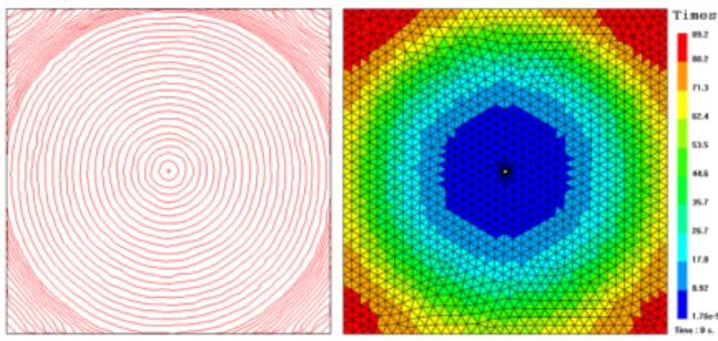
4.1 ISOTROPIC RADIAL INJECTION
We consider here the standard case of an isotropic radial injection, for a 0.25 m2square plate. The resin enters the
part from the center and flows through the preform de-scribing circular patterns. Four vents located on the cor-ners ensure the complete filling. Material and processing parameters are summerized in Tables 1 and 2.
Table 1: Material data
K[m2] µ[P a.s 1] ⇢[kg.m 3] ✏[ ]
1.10 9 0.1 1150 0.5
Table 2: Processing data
p0[P a] pf[P a] r0[m] g[m.s 2]
2.105 1.105 2.5.10 3 9.81
In the first case, gravity is neglected for a comparison with an analytical solution [1, 10]. It is given as
r f r0 2 . 2 ln✓rf r0 ◆ 1 + 1 =4K (p0 pf) t ✏µr2 0 (17)
where rfand r0are the radii of the moving front and the
inlet gate, p0 and pf the inlet and outlet pressures. The
mold is meshed using 2500 triangle elements. CPU time is around 20 s on a 2.26 GHz / 1.93 Go of RAM laptop. The predicted filling time is 98 s. Our model is assessed by fit-ting the numerical fronts using the analytically predicted circles. Figure 1 shows the comparison between our nu-merical results (left) and the analytical results (right). An-alytical results (in bold lines) are overlaid on our results, for 10.7 s and 63.3 s elapsed time. Using L1 norm leads to the relative error of 2.1%, which shows the accuracy of our numerical model.
Figure 1: Comparison with analytical solution
The second case takes into account gravity effects. On Figure 2 we compare our results (left) with a FEM/VOF-based code (PAM-RTMTM) (right) using the same mesh.
As expected, the flow is slightly deported in the lower part of the plate. The predicted filling time is 101 s for our simulation and 89 s for PAM-RTMTM, which shows
a good qualitative accordance. The difference is due to the contact implementation which is different in Level Set (see Equation 16) and VOF. Further developements will improve the contact accuracy by refining the mesh on the mold wall.
Figure 2: Comparison with FEM/VOF (PAM-RTMTM)
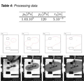
4.2 ANISOTROPIC INJECTION INVOLVING COMPLEX SHAPES
We compared our numerical results with experimental data, performing an infusion experiment involving a more realistic case. It consisted in impregnating an anisotropic knitted glass preform (1x1 rib knit fabric manufactured by Textile Aero Tarn) using a canola oil. The reinforce-ment (one layer) was placed under a transparent
flexi-ble bag and filled using two inlet gates and two vaccum lines (on the upper and lower sides). The dimensions of the mold are 0.3 m per 0.35 m. Some internal obstacles were placed to simulate contacts with mold walls. Mate-rial data (see reference [14] for measurement procedure) and processing parameters are given in Tables 3 and 4. CPU time is around 200 s for a model involving 3693 ele-ments. Figure 3 shows the comparison between our results (at the top) and experimental data (at the bottom) at differ-ent times.The agreemdiffer-ent is fair at any time. In particular, fronts merging (at 3 s) and dividing on the obstacles (at 7 s) are accurately predicted.
Table 3: Material data
K1[m2] K2[m2] µ[P a.s 1] ✏
1.50.10 9 7.75.10 10 0.067 0.705
Table 4: Processing data
p0[P a] pf[P a] r0[m]
1.03.105 120 5.10 3
Figure 3: Comparison with infusion experiment
5 CONCLUSION
We developed a software to predict a two-dimensional resin impregnation for both isotropic and anisotropic cases. Results were compared with an analytical so-lution, a FEM/VOF-based simulation and experimental data, with a fair agreement. The implemented model in-cludes a gravity term, but it can easily be modified to take into account other body forces. Further develope-ments will include a 3D approach (technique remains un-changed), and a high permeability layer to simulate infu-sion process.
ACKNOWLEDGEMENT
This work was supported by DAHER-Socata and CRCC. The authors are grateful to B. Cosson (ENSM Douai) and
M. Bordival (ICA-Albi) for their contributions.
REFERENCES
[1] F.M. Schmidt, P. Lafleur, F. Berthet, and P. Devos. Numerical simulation of resin transfer molding us-ing linear boundary element method. Polymer Com-posites, 20(6), december 1999.
[2] M-K. Um and L. Wi. A study on the mold filling pro-cess in resin transfer molding. Polymer Engineering and Science, 31(11):765–71, 1991.
[3] J.A. García, Ll. Gascón, E. Cueto, I. Ordeig, and F. Chinesta. Meshless methods with application to liquid composite molding simulation. Comput. Methods Appl. Mech. Engrg., (198) 2009.
[4] F. Trochu, R. Gauvin, and D-M. Gao. Numeri-cal analysis of the resin transfer molding process by the finite element method. Adv Polym Technol, 20(6):329–42, 1993;12(4).
[5] C. W. Hirt and B. D. Nichols. Volume of fluid (vof) method for the dynamics of free boundaries. Jour-nal of ComputatioJour-nal Physics, 39:201–225, January 1991.
[6] J.A. Sethian. Level Set Methods and Fast March-ing Methods EvolvMarch-ing Interfaces in Computational Geometry, Fluid Mechanics, Computer Vision, and Materials Science. Cambridge University Press, 2nd edition, 1999.
[7] S. Soukane and F. Trochu. Application of the level set method to the simulation of resin transfer mold-ing. Composites Science and Technology, 66:1067– 1080, 2006.
[8] Y-E. Yoo and L. Wi. Numerical simulation of the resin transfer mold filling process using the boundary element method. Polymer Composites, 17(3):368–74, 1996.
[9] P. Simacek and S.G. Advani. Role of acceleration forces in numerical simulation of mold filling pro-cesses in fibrous porous media. Composites Part A, 37:1970–1982, 2006.
[10] K.L. Adams, W.B. Russel, and L. Rebenfeld. Ra-dial penetration of viscous liquid into a planar anisotropic porous medium. International Journal Of Multiphase Flow, 14(2), 1988.
[11] C.A. Brebbia and J. Dominguez. Boundary ele-ments: an introductory course. McGraw-Hill Com-pany: Computational Mechanics Publications, 2nd edition, 1992.
[12] E. Mathey. Optimisation numérique du refroidisse-ment des moules dinjection de thermoplastiques basée sur la simulation des transferts thermiques par la méthode des éléments frontières (in French). PhD thesis, 2004.
[13] J.A. Sethian and P. Smereka. Level set methods for fluid interfaces. Annual Review of Fluid Mechanics, 35:341–372, 2003.
[14] G. Dusserre, E. Jourdain, and G. Bernhart. Effect of deformation on knitted glass preform in-plane per-meability. (Submitted to) Polymer Composites.