Principal Static Wind Loads on a large roof structure
Nicolas Blaise
a, Lotfi Hamra
a, Vincent Denoël
aa
University of Liège, Structural Engineering Division, Liège, BELGIUM
ABSTRACT
Usually, structural wind design is realized using static wind loads. Such loadings are expected, as a main property, to recover by static analyses, the envelope values that would be obtained by a formal buffeting analysis. For simple structures, equivalent static wind loads might be used but they are established in order to reproduce envelope values of specific structural responses and are thus not suitable to reconstruct efficiently the entire envelope. Recently, more general methods were derived to propose global static loadings that reconstruct the entire envelope but several drawbacks remained as their robust applicability for any structure and accuracy.
This paper addresses a new type of static loadings, the principal static wind loads, derived in a strict mathematical way, the singular value decomposition, to make it optimum for the envelope reconstruction problem. The method is illustrated with a large roof and the reconstruction accuracy is analysed by studying the rate of envelope reconstruction, envelope previously obtained by a rigourous stochastic analysis. The way principal loadings are derived makes them suitable for combinations in order to increase the rate of the envelope reconstruction. As a major outcome, the method provides a finite number of design load cases that matches a desired level of accuracy in the envelope reconstruction.
KEYWORDS: Buffeting wind analysis; envelope value; extreme value; equivalent static wind loads; singular value decomposition.
1. INTRODUCTION
The design of structures loaded by Gaussian wind loads can be realized using different approaches. For usual structures, static wind loads are provided in codes and might be used for the design if several assumptions are fulfilled. If not, dynamic buffeting analysis has to be performed and the envelope values, minimum and maximum, of any internal force may be established for the structural design. Nonetheless, structural engineers are still used to design with static wind loads. Indeed, such loadings may be combined with other codified static loads such as self-weight or snow.
This issue is stated as the envelope reconstruction problem and formulated as follows: given the envelope of internal forces obtained with a formal dynamic buffeting analysis, find the most appropriate set of static wind loads that accurately reconstruct, by static analyses, the real envelope with a high reconstruction rate.
This envelope reconstruction problem has already been addressed with different techniques such as universal loads (Katsumura et al., 2007), proper-orthogonal decomposition of wind loads (Fiore & Monaco, 2009) or least-squares fitting (Zhou et al., 2011). A drawback of the aforementioned methods is their applicability to any structure. Moreover they focus on the aerodynamic loading and therefore do not include the structural behavior of the structure. This paper addresses a new type of design loadings, the Principal Static Wind Loads (PSWLs), recently introduced by Blaise & Denoël (2012).
First, the formal buffeting wind analysis is described and the formulation of the PSWL is given. Then follows an illustration with a description of the considered structure, a summary of the wind tunnel simulations and results of the present study where the optimality of the PSWL basis for the envelope reconstruction problem is illustrated.
2. BUFFETING WIND ANALYSIS
For a given oncoming wind direction, the measured aerodynamic pressures qtot(t) are expressed in the full scale and adequately transformed to nodal external forces ptot(t) for the finite element (FE) analysis. The mean part µp is computed and the fluctuating part p(t) is
defined such that: p
µ
ptot = p + . (1)
The structural displacement satisfies the equation of motion:
p Kx x C x
M&&+ &+ = (2) where M,C and Kare the mass, damping and stiffness matrices, respectively, x(t) is the nodal displacements and the dot denotes time derivative.
The structural responses r(t) (internal forces, stresses or reactions) are considered here expressed by linear combinations of the nodal displacements
Ox
r = (3) where O is a matrix of influence coefficients, known from the FE model. The structural design needs envelope values (minimum and maximum) of the structural responses which are computed here as expected values of extrema on 10-minute observation windows. The envelope
(
rmin,rmax)
is defined asr max r min g ; gσ r σ r =− = (4)
where σr is the standard deviation of the structural response and g is a unique peak factor taken equal to 3.5. For simplicity, standard deviations of the structural responses are obtained from the covariance matrix of the nodal displacements C using x
) (
diag x T
r OC O
σ = (5) where diag is a matrix operator that keeps only the diagonal of the matrix. Application of the well-known Background/Resonant decomposition concept leads to a covariance matrix C x
composed of two uncorrelated respective contributions x(B) and x(R)
(R) x ) B ( x x C C C = + . (6) The covariance matrix of the background contribution of the nodal displacements (B)
x C is given by: -T p (B) x K C K C = -1 (7) where C is the covariance matrix of the nodal forces. p
The dynamic analysis, necessary to establish (R)
x
C , is performed efficiently by solving Eq.2 in the modal basis, i.e. assuming
) R ( ) R ( φη x = (8)
where η(R)(t) is the resonant contribution of the modal displacements and φ is the modes
shapes. The PSD matrix of η(R)(t) is obtained as:
T ) wn ( p ) R ( * * *S H H Sη = (9)
where H* =
(
−ω²M*+iωC*+K*)
−1 is the modal transfer function with * * C ,M and K* the
generalized mass, damping and stiffness matrices, respectively and (* )
wn p
S is the equivalent white noise matrix of the generalized forces (Denoël, 2009). The covariance matrix of the resonant contribution of the nodal displacements (R)
x C is obtained by T ) R ( T (R) ) R ( x φC φ φ S ( )d φ C
∫
+∞ ∞ − = = η η ω ω (10)Ultimately, the design of the structure is based on the design envelope
(
rd,min,rd,max)
defined as max r max , d min r min , d µ r ; r µ r r = + = + (11)where µr =Aµp is the mean part of the structural responses and A is a matrix of influence
coefficients.
In this paper, we focus on the most critical wind direction for the structural design, i.e. the wind direction that would provide the largest reconstruction of the design envelope obtained
after considering the buffeting analysis for all wind directions. 3. ENVELOPE RECONSTRUCTION USING STATIC WIND LOADS
The main objective of this paper is to reconstruct the envelope
(
rmin,rmax)
obtained with theprevious buffeting analysis, see Eq.4, using a limited number of well-suited static wind loads. First, Equivalent Static Wind Loads (ESWLs) pe are computed for each structural response
max
r of interest using the method developed by Chen & Kareem, 2001. All of these equivalent loadings are collected in a matrix Pe factorized by Singular Value Decomposition
' SV P
Pe= p (12) where p
P is the matrix of Principal Static Wind Loads (PSWLs), the matrix S collects, on its main diagonal, the principal coordinates and the matrix Vcollects the combination coefficients to reproduce the ESWLs. The SVD operation extracts the principal components of the ESWL basis and thus represents, by order of importance, the main loadings which, by combinations, can produce any extreme structural response. Each principal loading ppj is normalized such that the static response
p p p j p j Ap ; R AP r = = (13) is somewhere tangent to the envelope
(
min max)
,r
r .
The way to define PSWLs suggests that linear combinations may be considered. Any combination of the PSWLs produces a new static loading denoted p . It is associated with s
(a) (b) s s p p s Ap r q P p = ; = (14) where q is a vector of combination coefficients. p
The successive static analyses under each combination of the principal loadings produce a sequential symmetrical reconstruction of the envelope
(
~rks,min,~rks,max)
defined as(
~ ; ; ;0)
; ~ max(
~ ; ; ;0)
min ~ s,max s s 1) (k max s, k s s min s, 1) (k min s, k r r r r r r r r = − − = − − . (15) Because the envelope(
rmin,rmax)
is symmetric, with the thk reconstructed envelope is associated 2k loading cases.
Finally, the accuracy of the envelope reconstruction is assessed by the relative errors computed as min min min , s k max max max , s k k ~ ~ r r r r r r − = − = ε (16)
where the division is performed element by element. 4. ILLUSTRATION
4.1. Description of the structure
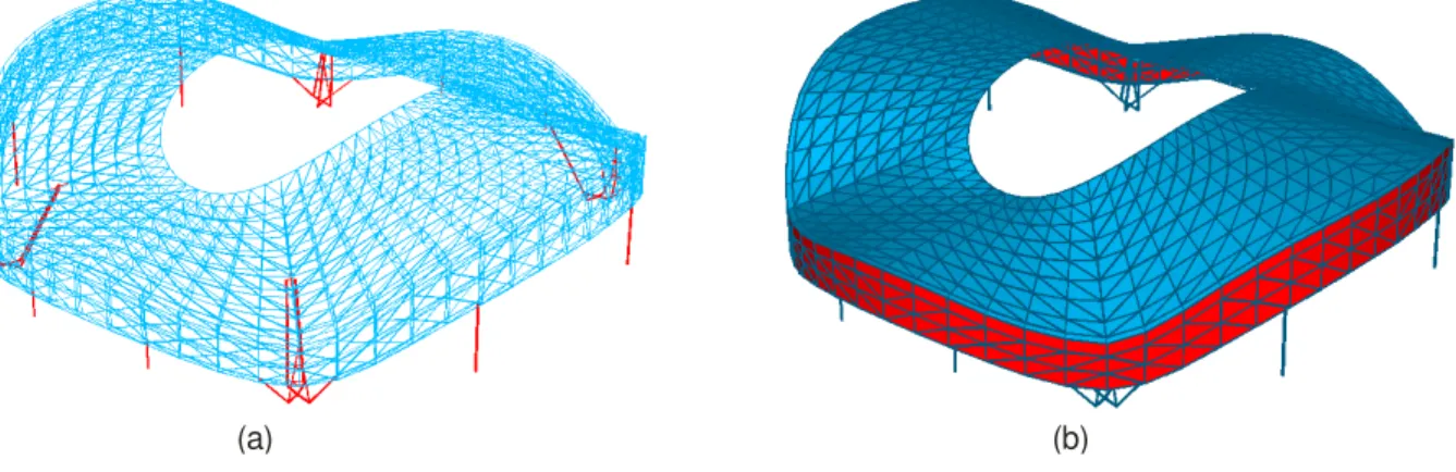
The considered structure is the roof Marseille’s velodrome in France which will undergo serious rehabilitations in 2013. Figure 1-(a) shows the FE model with the supports in red and the structural truss supporting the roof (in blue) and Fig.1-(b) shows the upper roof in blue and the vertical sheeting (in red). The dimensions are 258x256x74 meters.
Figure. 1. (a) Structural finite element model and (b) roof composed of a high density polythene membrane.
The structure is a rigid lattice composed of hollow tubes and the roof is covered with a high density polythene membrane. Table 1 gives the main characterstics of the 3D finite element model.
Table 1. Characteristics of the 3D finite element model.
Number of elements 7071 Number of types of elements 5 Number of geometries 107
Number of beam elements 5736 Types of material 2 Number of nodes 1896
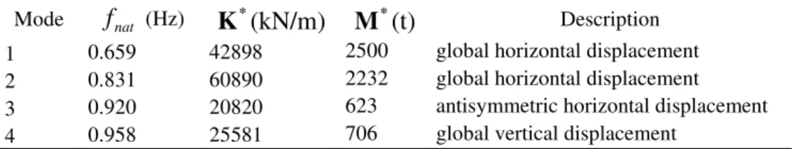
The fundamental mode has a frequency of 0.66 Hz and only the first four modes are kept for the buffeting analysis because they have their natural frequencies lower than the Nyquist frequency, see section 4.2. Techniques to consider more modes for the buffeting analysis have
been applied by Hamra (2012) but are not shown here for sake of consiceness. Table 2 gives the natural frequencies, the generalized stiffness and mass for the first four modes.
Table 2. Natural frequencies, generalized stiffness and mass for the first four modes. Mode fnat (Hz)
*
K (kN/m) M (t)* Description
1 0.659 42898 2500 global horizontal displacement
2 0.831 60890 2232 global horizontal displacement
3 0.920 20820 623 antisymmetric horizontal displacement
4 0.958 25581 706 global vertical displacement
Figure 2 depicts the modal displacements of the first and third modes. The first one is a global horizontal displacement and the third is an antisymmetric horizontal displacement one. The structural damping ratio is considered equal to 1% for each mode.
Figure 2. Mode shapes of (a) the first and (b) the third modes.
4.2. Wind tunnel simulation
The aerodynamic loading characterization has been realized by wind tunnel simulations at the “Centre Scientifique et Technique du Bâtiment” at Nantes, France. Twenty-two wind directions have been tested including the four wind directions perpendicular to the two principal axes. Table 3 collects the target wind properties and the given values corresponding to the Service Limit State.
Table 3. Main wind properties of the wind characterization. Reference wind velocity
0 , b
v 26 m/s Height of the structure zs 62 m Values for Cdir=1,]210°;50°[
Season factor cseason 1 Terrain category IIIb z0 0.5 m Mean velocity wind vm( )zs 28 m/s
Directional factor
dir
C [50°;210°] 0.85 Roughness factor kr 0.2232 Turbulence intensity Iv( )zs
19,1 %
Directional factor
dir
C ]210°;50°[ 1 Ground factor cr(zs) 1.076
Reference velocity pressure
( )s mean z q 479 N/m² Orography factor c0 1
Peak velocity pressure
( )s p z
q
1122 N/m²
Figure 3-(a) shows the 1/250-scaled model and its environnement within a 475 meter radius. The future buildings in the project are also realised and localized in red on Fig.3-(b). The model is considered to be infinitely rigid. The scaled model was instrumented with approximatively five hundred synchronous pressure sensors. The sampling frequency is equal to 200 Hz, which corresponds to 2.2 Hz in full scale. This paper focuses exclusively on the most restrictive wind direction: 220°, see section 4.3.
Figure 3. (a) Scaled model of the stadium and its environement tested in the wind tunnel and (b) map view with the future buildings in the project (in red).
4.3. Results
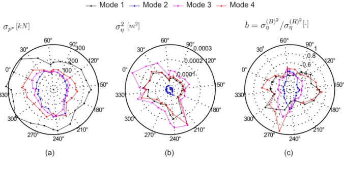
Figure 4 shows results for the first four modes for the twenty-two wind directions tested. Figure 4-(a) shows the standard deviations of the generalized forces. The fundamental mode presents the highest values and in general, the sector [50°; 210°] gives lower standard deviations for any mode which is a consequence of the reduced directional factor adopted. Figure 4-(b) shows the variance of modal amplitudes. The third mode has the highest modal amplitude, the fundamental mode and the fourth have close values while the second mode has small values. This is partially explained by the generalized stiffness, see Tab.2. For the 220° wind direction, the third and fourth modes show large va riances simultaneously. Figure 4-(c) depicts the background-to-resonant ratios to assess the structural behaviour of the structure. The coefficients take only values under one with smaller values for the 220° wind direction which corresponds to a clearly resonant behaviour of the structure under wind actions.
The choice of the studied wind direction (220°) is based on the mean relative errors
(
d,max)
i min , d i ,EE between the design envelope obtained for a wind direction and the design
envelope if all wind directions were considered
(
)
(
)
r N k kid,max i max , d ki i max , d ki max , d r N k kid,min i min , d ki i min , d ki min , d i /N ) r ( max r max r ; N / ) r ( min r min r r r∑
∑
− = Ε − = Ε i (17)where rkid,min and rkid,min represent the design envelope values (minimum and maximum) of the
th
k structural response for the ith wind direction and Nr is the number of studied structural
responses. The envelope considered for the reconstruction problem collects the six internal forces (axial force, two bending moments, two shear forces and torque) for all of the beam elements, given a r
N equal to 68832. Indeed, all types of internal forces are considered
without any distinction to handle the envelope reconstruction problem.
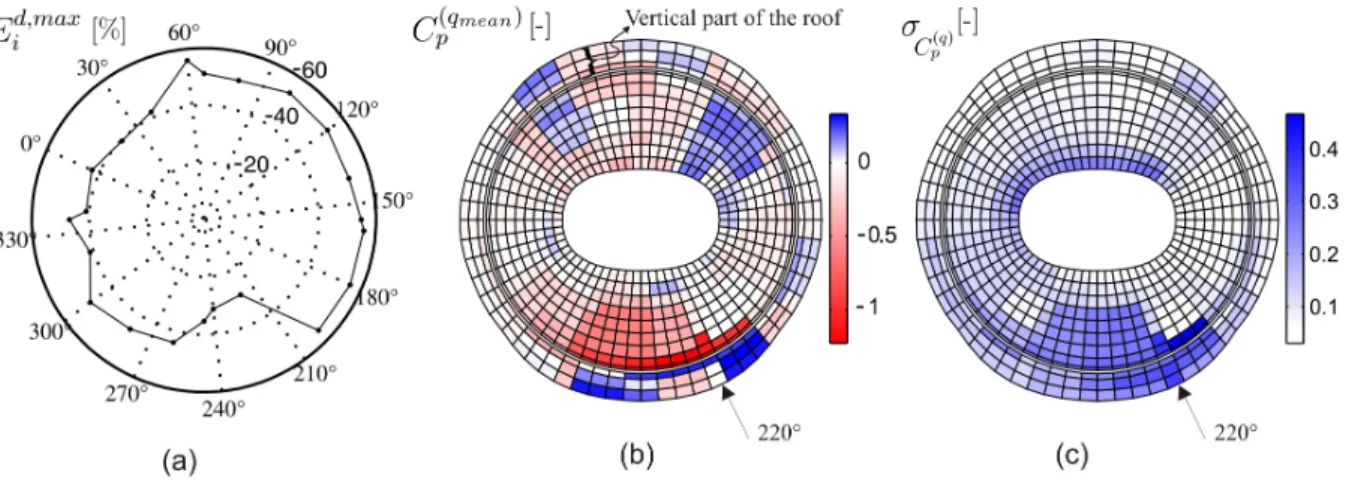
Figure 5-(a) shows the mean relative errors of the maximum part of the design envelope
max , d
E . It indicates that the 220° wind direction produces the lowest value: approximatively
-30%. For sake of brevity, the envelope reconstruction problem is demonstrated for this wind direction only. Assessment of the aerodynamic loading is made through the dimensionless pressure coefficient C(pqtot) defined from
) q ( p ) q ( p s mean s mean q ) q ( p C C ) z ( q q ) z ( q C tot = µ + = mean + (18)
with C(pqmean) its mean part and (q) p
C its fluctuating part. Figure 5-(b),(c) show the maps of
) q ( p mean
C and standard deviations of the fluctuating part of the pressure coefficients C(pq). Notice that an exploded view of the vertical sheeting, see Fig.1-(b), is represented in the Fig.5-(b),(c). As expected, the windward side of the roof is mainly in depression (with reference to the atmospheric pressure and associated to negative values) with higher values close to the sharp edge connection with the vertical part of the roof where exists zones with positive pression. Standard deviations may be explained by the vortex shedding intensity which is important on the windward side of the roof because the air flow encounters the structure’s roof with its sharp edge connection between the horizontal and vertical parts. Also, important standard deviations are noticed at the leeward side of the inside perimeter of the roof where layer separation and vortex shedding take place.
Establishment of the PSWLs basis needs to first compute 68832 ESWLs and then to apply the SVD operation on them.
Figure 5. (a) Mean relative errors of the maximum part of the design envelope for each wind direction, (b) mean and (c) standard deviations of the pressure coefficients for the 220° wind direction.
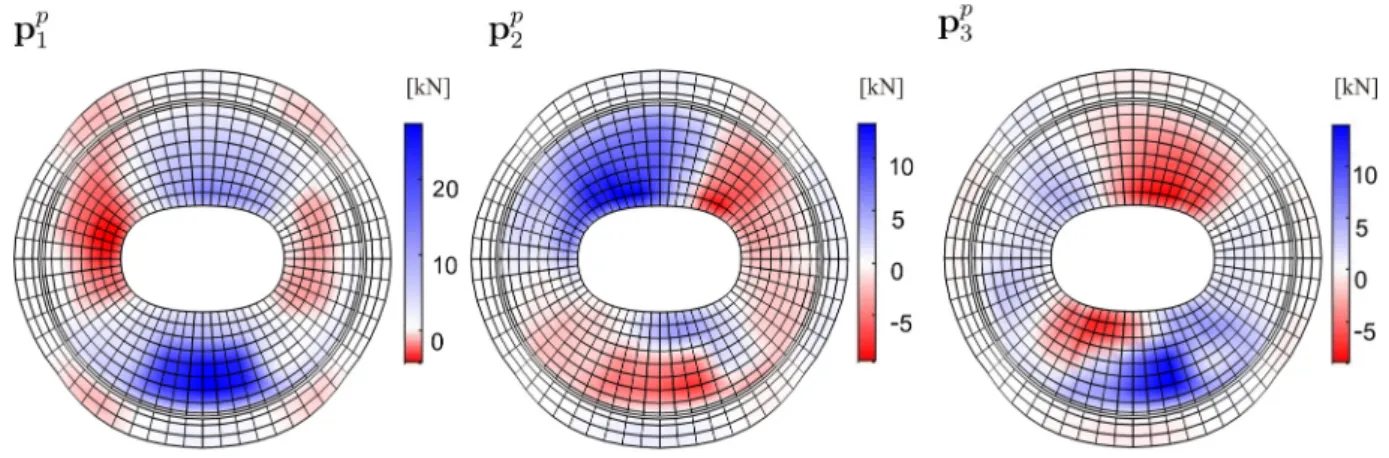
Figure 6 depicts the global vertical external forces of the first three principal static wind loads. Because all structural responses have been taken into account, these principal loadings present large zones of loadings on the entire roof which indicate that they are appropriate for the global entire envelope reconstruction problem.
Figure 6. First three principal static wind loads. Global vertical external forces.
Figure 7-(a) shows the principal coordinates for the first twenty principal loadings. They are ordered by decreasing importance which indicates that only the first few M PSWLs may be representative for the envelope reconstruction problem.
The envelope reconstruction is first illustrated with 120 beam elements localized at the outside perimeter of the roof and identified in bold in Fig.7-(b). Figure 7-(c) depicts the real envelope of the axial forces N for these elements.
Figure 7. (a) Principal coordinates of the principal loadings, (b) identification of the 120 beam elements considered, (b) axial force envelope for these elements.
Figure 8 shows the principal responses under the first, second and fifth principal loadings (upper half of each graph) and the sequential reconstruction of the envelope (lower half of each graph).
Considering more principal loadings does not improve significantly the reconstructed envelope because no combination is considered.
Figure 9 shows the relative errors for the 11472 axial forces considering the first one, two and five PSWLs (without combination). With the first five principal loadings, each axial force is partially reconstructed with a large part that has a relative error larger than -50%. This indicates that the PSWLs target simultaneously all elements no matter the magnitude of their internal forces.
Figure 8. Principal static responses and envelope reconstruction (without combination of principal loadings).
Figure 9. Relative errors for axial forces considering the first one, two and five principal loadings if there is no combination between them.
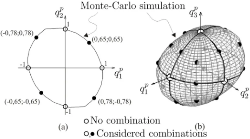
One interesting way to ameliorate the envelope reconstruction is to consider also combinations of principal loading rather than just their sequential application. Figure 10 depicts the curve and surface of coefficient sets which fulfill the tangency condition considering the first two (a) and three (b) principal loadings, respectively.
Figure 10. Scaled combination coefficients for (a) two PSWLs and (b) three PSWLs.
As indicated, the curve and surface are obtained by Monte-Carlo simulation. The circles represent the unitary coefficients for each PSWL taken independently from one another. Because Monte-Carlo simulation may become heavy to perform with the increase of the number of principal loadings, considered combinations are predefined. These combinations
are obtained by considering all possible combinations if each principal coefficient can take -1,1 or 0 values scaled to fulfill the tangency condition. The subspace of considered combinations counts 3M −1
different couple of coefficients.
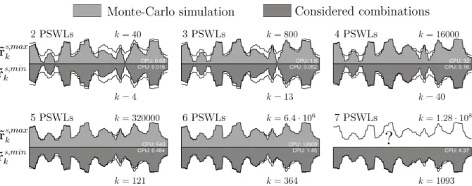
Figure 11 shows the max and min parts of the envelope that would be obtained by static analyses under combinations of principal loadings obtained by Monte-Carlo simulation and predefined, respectively. Random combinations of the first five principal loadings give an accurate reconstructed envelope. It also indicates that combination of principal loadings allows very good accuracy for the reconstructed envelope and also that within all possible couple of coefficients, only a fraction allow to further increase accuracy. So, clearly, the simple preselection we suggest is a smart tradeoff between accuracy & computational efficiency. The reconstructed envelope under random combinations of the first seven principal loadings is not shown because CPU time rapidly increases with the number of considered principal loadings.
Figure 11. Reconstructed envelope, max and min, obtained with combination coefficients of Monte-Carlo simulation (upper part of each graph) and considered combinations (lower part of each graph), respectively. CPU time in seconds.
Figure 12 allows to appreciate the gain of reconstructed envelope accuracy by combinations of principal loadings for all axial forces in the structure. In comparison with Fig. 9, the gain is impressive: considering combinations of the first three principal loadings gives better estimation than considering the first five principal loadings independently. Combination of the first five principal loadings offers a good accuracy of the reconstructed envelope, especially for the high values of axial forces. The reconstructed envelope with only the considered combinations of principal loadings is also accurate with, as expected, a slightly lower accuracy convergence than if all sets of coefficients were considered.
For design purposes, a finite number of representative design load cases has to be identified. A selection in the available set of combinations may be done based on the maximization of a choosen indicator of convergence. Such indicator of convergence
) , , ~ ( f k p p k = r−1r,p q Ψ (19) is defined as a function of the k−1th reconstructed envelope, the target envelope, the considered principal loadings and combinations thereof.
Figure 12. Relative errors for axial forces considering combinations between the first two, three and four principal loadings with coefficients obtained by Monte-Carlo simulation (upper part of the graph) or predefined (lower part of the graph).
If Nc is the number of available couples of coefficients, the best kth combinations (out of
c
N ) is the one that provides a Ψ optimum. k In order to illustrate the concept, let us define Ψk as the mean error of all structural responses:
∑
= Ψ r N l lk r k N ε 1 (20)where εlk is the relative error of the lth structural response in the kth reconstructed envelope.
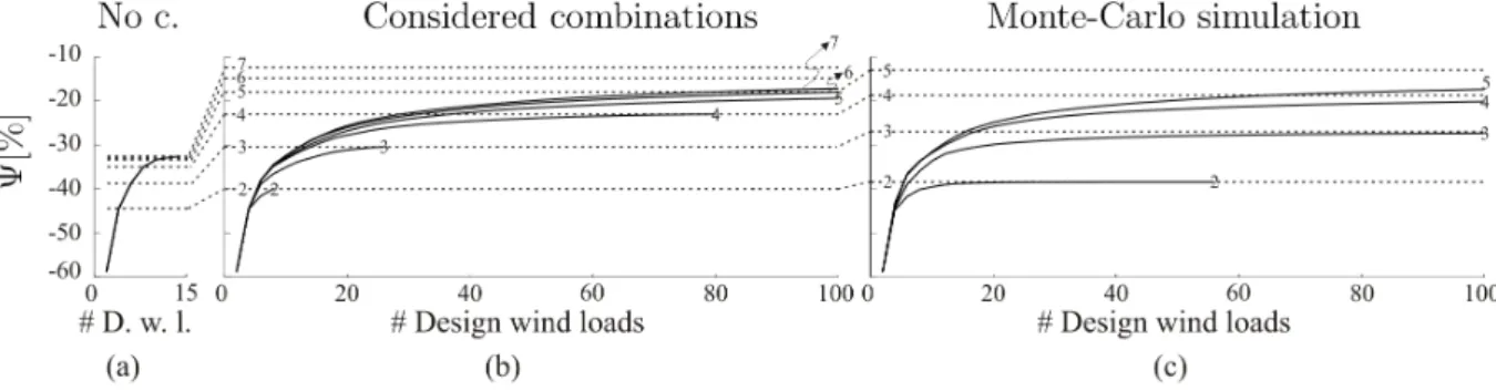
Figure 13 depicts the evolution of Ψ, function of the number of design wind loads derived with an increasing number of principal loadings, from two to seven, for each graph. The three graphs from left to right are the results if i) no combinations, ii) predefined considered combinations and iii) coefficients of Monte-Carlo simulation are used for the computation and selection of design wind loads. Dotted lines indicate the limit values for Ψ that would be obtained if all coefficients in the defined subspace of coefficients in the three approaches were considered. A rapid increase is observed with just the first few design wind loads, then followed by a transition zone where the slopes decrease with a slow monotonously convergence toward their respective limit values. Addition of principal loadings extends the transition zone and raise the limit values.
Figure 13-(a) illustrates that if no combination is considered, the limit values for Ψ are getting closer and thus consideration of more and more principal loadings does not bring improvement for Ψ.
Predefined considered combinations improves significantly the estimation of the envelope, as shown in Fig.13-(b) and the curves obtained are similar to the one if all possible coefficients were considered, see Fig.13-(c), with a slight negative shift.
Figure 13. Evolution of the indicator of convergence in function of the subspaces considered for the coefficients and the number of principal loadings.
Notice that, only results for two to five principal loadings are shown if the Monte-Carlo technique is used to establish the subspace of coefficients for combinations because the method is time-consuming. At the opposite, the considered combinations allows to study rapidly the convergence of the indicator for a higher number of principal loadings.
5. CONCLUSIONS
There are two important conclusions to be mentionned as a result of this work. First, a new basis of static wind loads, the principal loadings, has been successfully derived for a large roof structure. We found out that a very limited number of them are necessary for the envelope reconstruction problem. Secondly, the way there are defined makes them suitable for combinations in order to attempt a high level of reconstruction of the envelope with a limited number of loadings. Moreover, the proposed technique is adaptive through the indicator of convergence in order to meet specific envelope reconstruction requirements. ACKNOWLEDGEMENT
We would like to acknowledge the “Centre Scientifique et Technique du Bâtiment” in Nantes in France and also the design office “Greisch” in Liège, in Belgium for having provided the finite element model and the measurements in wind tunnel.
6. REFERENCES
Blaise N., Denoël V. (2012). Principal Static Wind Loads, Int. J. Wind Eng. Ind. Aerod., Under review. Chen, X. Z., Kareem, A. (2001). Equivalent static wind loads for buffeting response of bridges.
Journal of Structural Engineering-ASCE 127 (12), pp. 1467-1475.
Denoël V. (2009). Estimation of modal correlation coefficients from background and resonant responses. Structural Engineering And Mechanics 32 (6), pp. 725-740.
Fiore, A., Monaco, P., (2009). Pod-based representation of the alongwind equivalent static force for long-span bridges. Wind and Structures, 12 (3), pp. 239-257.
Katsumura, A., Tamura, Y., Nakamura, O. (2007). Universal wind load distribution simultaneously reproducing largest load effects in all subject members on large-span cantilevered roof. Int. J. Wind Eng. Ind. Aerod., 95 (9-11), pp. 1145-1165.
Lotfi H. (2012). Simplification du chargement aérodynamique sur une toiture de stade. Application : le vélodrome de Marseille. Travail présenté en vue de l’obtention du grade d’Ingénieur civil construction à finalité approfondie, Faculté des Sciences Appliquées, Université de Liège (2012). Zhou, X., Gu, M., Li, G. (2011). Application research of constrained least-squares method in
computing equivalent static wind loads. In: Proceeding of the 13th International Conference on Wind Engineering.