Application of a density current model to aircraft observations of the New England coastal front

APPLICATION OF A DENSITY CURRENT MODEL TO AIRCRAFT OBSERVATIONS OF

THE NEW ENGLAND COASTAL FRONT

by

PETER PAUL NEILLEY B.S., McGill University

(1982)

SUBMITTED TO THE DEPARTMENT OF

EARTH, ATMOSPHERIC AND PLANETARY SCIENCES IN PARTIAL FULFILLMENT OF THE

REQUIREMENTS FOR THE DEGREE OF

MASTER OF SCIENCE

at the _{O~ ~U:;~'}

MASSACHUSETTS INSTITUTE OF TECHNOLOGYWITHDRAN

May 1984

FROM

MIT LIBRAfrgn

Signature

Certified

of Author

Department of EarthdAtmospheric a d Planetary Sciences

''

May 1984

-2-APPLICATION OF A DENSITY CURRENT MODEL TO

AIRCRAFT OBSERVATIONS OF THE NEW ENGLAND COASTAL FRONT by

PETER PAUL NEILLEY

Submitted to the Department of Earth, Atmospheric and Planetary Sciences

in partial fulfillment of the requirements for the degree of Master of Science in Meteorology

ABSTRACT

The vertical structure of the New England coastal front is determined using aircraft observations. The coastal front is found to be an extremely narrow transition zone between two distinct air masses. Horizontal temperature gradients as large as 12.9 C km- 1 with wind shifts of nearly 180 deg in 200 m

horizontal distance were found across the front. A vertical jet of about 1.5 m s-1 _{characterizes the front and there is evidence}

that this updraft directly enhances the observed precipitation field downstream. The overall structure of the coastal front is found to be similar to a two-fluid density current.

Thesis supervisor; Dr. Richard Passarelli Title: Assistant Professor of Meteorology

-3-INDEX ABSTRACT... INDEX... LIST OF FIGURES... CHAPTER I: INTRODUCTION... CHAPTER II: STRUCTURE OF THE FRONT... A. Case of 10 January 1983... B. Case of 15 January 1984... CHAPTER III: THE DENSITY CURRENT ANALOGY CHAPTER IV: SUMMARY AND DISCUSSION... APPENDIX... ACKNOWLEDGEMENT... LIST OF REFERENCES... 1. 2. 3. 4. 5. 6. 7. 8. 9. 10. 2 3 4 6 12 12 31 48 55 59 62 .63

-4-LIST OF FIGURES

1. Surface analysis of the eastern U.S. January 1983...

2. Surface analysis of eastern New January 1983... at 1200 GMT on 10 ... ... ... 13 England at 1800 GMT 10 ... . ... 15

3. Raw aircraft data of a) temperature, b) dew point temperature c) wind speed and d) wind direction taken during the 15 M AGL pass through the front on 10 January 1983...17

4. Same as 3 a-d except the data are from through the front...

5. Cross section of potential temperature the coastal front of 10 January 1983..

the 450 m AGL pass ... 18

(*C) and winds for ... 20

6. The stream function normal to the coastal front of 10 January 1983...23

7. Comparison of vertical gust measured by the aircraft with that calculated from the stream function...27

8. Cross section of the wind speeds parallel to the front for the 10 January 1983 case...29

-5-9. Surface analysis of eastern New England at 1500 GMT on 15 January 1983... ...--- 32

10. Raw plots of a) temperature, b) dew point

c) wind speed and d) wind direction taken AGL pass through the coastal front on 15

temperature, from the 150

January 1983...34

11. Same as 10 except that the data are from the 450 m AGL pass through the front... 35

12. Cross section of potential temperature (0 C) of the 15

January 1983 coastal front...37

13. Stream function corresponding to 12...38

14. Parallel winds corresponding to 12...39

15. Mean precipitaion rate (mm/hr) plotted normal to the front for the 15 Jannuary 1983 case ...

16. Calculated snowflake front of

trajectories near the coastal

15 January 1983...45

17. Skematic diagram of a typical laboratory density

current...50 ... 43

-6-CHAPTER I INTRODUCTION

Coastal frontogenesis in eastern New England has not been well understood partially because of the lack of a detailed observational study of the phenomenon. To help overcome this deficiency, the New England Winter Storms Experiment (NEWSEX)

conducted by the Center for Meteorology and Physical Oceanography at MIT has had as one of its primary objectives the acquistion of detailed observations of the New England coastal front. The purpose of this paper is to present an analysis of some of the results of this effort. It will be shown that the coastal front exhibits dramatic contrasts in just over 200 m horizontal distance of both the thermodynamic and kinematic variables. The coastal front will also be shown to resemble a classical two-fluid density current.

The New England coastal front was first documented by Bosart et al. (1972). They present a series of case studies of a mesoscale boundary layer frontal zone, often no wider than 10 km, exhibiting large contrasts in temperature and wind. The frontal band normally extends several hundreds of kilometers along the New England coastline and hence the name. They note however,

-7-that the front often forms as far as 50 km inland from the shoreline, especially in southeastern New England between Boston and Providence.

Using detailed surface analysis, Bosart et al. found cross-frontal temperature contrasts between 5 and 10 C, with the cold air always lying on the inland (west) side. Cyclonic wind shear from weak (< 5ms-1 ) northerly in the cold air to strong (5-10 ms-1) easterly or southeasterly in the warm air is found across the front. Precipitation sometimes accompanies the front with a change in form across the front sometimes occuring (e.g. from rain to freezing rain or snow).

With respect to the synoptic conditions, Bosart et. al. found that coastal frontogenesis can commence 6 to 12 hours after the establishment of a cold V-shaped high pressure ridge in northern New England. The coastal front typically persists for a period of 12 to 24 hours thereafter. The dissipation of the front is triggered by the arrival of a cyclone from the southwest which causes the winds to become uniform on both sides of the front.

Bosart (1975) later studied in greater detail the synoptic scale conditions that are conducive to the formation of a coastal front in New England. He found that coastal frontogenesis is always associated with a high pressure ridge extending into and receding from New England. Along with this ridge, he also found that a deep but filling cyclone in the Ohio valley and a secondary cyclone forming off the Carolina coast are most often

-8-associated with the onset of coastal frontogenesis. The secondary cyclone usually grows rapidly as it moves toward New England and often becomes the dominant weather feature in the northeast. Most of the other synoptic scale conditions that Bosart found with coastal frontogenesis are mainly distinquished by differences in the strength and position of the two cyclones.

The nature of the V-shaped ridge that seems to be essential for coastal frontogenesis was studied by Baker (1970). He showed that the ridge is the result of a pool of dense cold air that has become dammed up against the eastern slopes of the Appalachian Mountains by a large-scale easterly geostrophic forcing. The surface winds under the ridge are usually northerly as the cold air drains along the mountains toward lower pressure.

Bosart (1975) also compiled a climatology of coastal frontogenesis from eight years of data. He found that an average of eight New England coastal fronts form each year but he indicated that this number is probably too low. He noted that the vast majority of coastal fronts occur in the late fall and early winter, coincident with the maximum contrast in land-sea surface temperatures.

Bosart et al. (1972) argued that the effects of differential surface friction, coastal configuration, orography and land-sea temperature contrast are important factors in coastal frontogenesis. Bosart (1975) found that coastal frontogenesis occurs when onshore geostrophic winds forced by the receding anticyclone converge near the coastline, probably because of

-9-differential surface friction. Provided that there is a pre-existing surface temperature gradient, presumably set up by the land-sea temperature contrast, coastal frontogenesis, he argued, will occur as isentropes collapse together in the convergence zone.

Ballentine (1980) conducted a numerical experiment on coastal frontogenesis using a highly specialized boundary layer model. For real data initializations, he could produce a coastal front only when the synoptic scale geostrophic wind took on an easterly component. Further, by varying the parameterization of surface heat flux, differential friction, orography and latent heat release, he concluded that the flux of heat out of the ocean is the primary physical process leading to frontogenesis along the coastline. The other factors were determined to be secondary.

McCarthy (1977) studied the upper air structure in the vicinity of the coastal front. Using the standard upper air observations and pertinent surface observations, he constructed cross sections through the coastal front. He found that the typical coastal front environment consists of three layers of air, each having a different character and origin. The lowest layer west of the surface frontal position is a cold continential air mass characterized by high stability, northerly or northeasterly winds less than 5 ms- 1, and low relative humidity

(except possibly during precipitation). This layer is generally less than 750 m thick. Above and east of this layer is a warmer

-10-less stable maritime air mass. This air is, or has recently been in direct interaction with the ocean and therefore has a higher moisture content. Winds in this layer are generally east to

southeast at 5 to 10 ms- 1. A synoptic-scale warm frontal inversion lies above this layer, typically at a height of 1 km, and forms the boundary into the third air mass. This top layer has the highest relative humidity and south or southwest winds usually stronger than 10 ms- 1. McCarthy noted that the height of the warm frontal inversion depends upon the position of the approaching cyclone and sometimes descends to the surface, displacing the coastal front.

Along the frontal interface, a vertical jet may occur in response to the convergence of the horizontal winds. Provided

that this jet is strong and deep enough, an area of enhanced precipitation at and west of the surface frontal position should occur. Indeed, this enhancement has been noted in varying degrees by Bosart et al. (1972) and Bosart (1975) from surface observations, by Marks and Austin (1979) using radar, by McCarthy from satellite images and by Ballentine using his numerical model. Bosart et al. (1972) also noted that because of the large temperature contrast, the coastal front often marks the boundary between frozen and non-frozen precipitation. Freezing rain, sleet and snow have all been observed west of a coastal front while rain was falling to the east.

-11-Accurate weather forecasting in eastern New England certainly depends upon careful consideration of the possibility of coastal frontogenesis. Still, even the most careful forecasts are subject to large errors in temperature and precipitaion because of the uncertainties in where and when the coastal front will form, and how persistent and how intense it will be. Evidently, significant forecasting improvements will depend upon the degree to which the coastal front is further understood. Many questions still remain to be answered before this goal can be achieved. For instance, in regard to the front's structure: How narrow is the actual frontal zone? What type of vertical circulation is driven by the front? Would this vertical circulation be able to account for any observed precipitation enhancement? In regard to the mechanics of the front: What role does rotation play in the frontogenesis mechanism? Finally, what determines where the front will form and how it will move? Following are two case studies that attempt to answer some of these questions and point towards the answers for others.

-12-CHAPTER II

STRUCTURE OF THE COASTAL FRONT

The primary data used in this study were collected with NCAR's instrumented Queen-Air aircraft loaned to MIT during NEWSEX. In addition to measuring the standard meteorological parameters, the plane is equipped to determine cloud and precipitation particle-size distributions with Particle Measuring Systems (PMS) probes. The position of the aircraft is determined

by an inertial navigation system (INS). All parameters are sampled once per second, yielding a horizontal resolution of about 70 m at normal cruising speeds.

Two significant coastal fronts were studied during the operational period of NEWSEX in the winter of 1982-1983. Individual case studies of each are presented here.

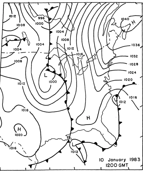
1. Case of 10 January 1983. The synoptic conditions in the eastern U.S. during the early morning of 10 January 1983 are shown in Fig. 1. These conditions are nearly identical to those which Bosart (1975) found most often associated with coastal frontogenesis. A 1040 mb anticyclone became established northeast of New England on the previous night with a ridge extending southwest along the Appalachians. A deep low was moving northeast out of the Midwest and by 1200 GMT (7 am LST) on the 10th, a new low had developed off Cape Hatteras. Radiational cooling throughout much of the previous night allowed a strong

-13-Fig. 1. Surface isobaric analysis in the eastern US at 1200 GMT on 10 January 1983.

-14-land-sea surface temperature gradient to develop in eastern New England. A coastal front began to form by 0900 GMT and was well

established along the eastern New England coastline by 1500 GMT. Fig. 2 presents the surface analysis of eastern New England at 1800 GMT. It is constructed using all available observations

including Coast Guard reports. The Coast Guard observations do not include cloud cover and are thus plotted with an "M". The coastal front can be seen to run from central Connecticut northeastward to just west of Boston and then northward along most of the New Hampshire and Maine coastline. This is typical of the New England coastal front (see e.g. Bosart et al.).

The aircraft took off from Bedford MA (BED) at 1630 GMT on the morning of the 10th. Portsmouth NH (PSM) was selected as the observing area because of its proximity to the front and the relatively sparse air traffic. The aircraft arrived on location by 1700 GMT and proceeded to make six 40 km passes centered on the front at the approximate altitudes of 151, 100, 150, 250,

350, and 450 m AGL. The aircraft maintained a true heading of

150*-330* which at the time was thought to be perpendicular to

the front. The data collection was confined as closely as possible to one vertical plane. The coastal front was encountered about 15 km southeast of Portsmouth, or about 7 km offshore. The entire set of observations took about 90 min.

1 Over water the flight track was indeed this low. However when the track passed over land the aircraft was forced to fly somewhat higher. However, since the coastal front was encountered over the ocean, it was, in fact, penetrated at about 15 m ASL.

-15-720 71* 70*

Fig. 2. Surface analysis in eastern New England at 1800 GMT

(1 pm LST) on 10 January 1983. Isobars are drawn every 2 mb and isotherms are drawn every 2.5*C. Wind barbs are in knots. Coast guard reports are plotted with a "M".

-16-By the time the observations were taken, the skies had become overcast with a stratocumulus deck estimated to have a 1.2 km base. There were a few breaks in the clouds on both sides of the front but these were more than 20 km away from the surface frontal position. There were no other obvious features noted by the flight observer (the author) in the cloud structure near the front, and there was no precipitation.

Figs. 3 a-d are raw plots of temperature, dew point, wind speed and wind direction for the lowest pass through the coastal front. The coastal front is clearly depicted in these plots as a sudden jump in temperature and change in the wind direction. Most of the large jump is represented by just three seconds of data. This rapid transition presses the response sensitivity of some of the instruments, particularly of the dew point measurement instrumentation. The total change in temperature across the coastal front is 9 C, of which more than half occurs at the jump. The wind shift occurs almost exclusively at the front and amounts to 180 deg over 200 m horizontal distance. Note that the parameters are generally flat on the warm air side of the front but have a definite slope in the cold air. The dew point trace shows a sudden rise ahead of the front, exactly

coincident with the position of the shoreline.

Figs. 4 a-d are identical to the plots of Fig. 3 except that the data are from the the highest (~ 450 m AGL) pass through the front. The front at this height is marked only by a slight transition in temperature of less that 1 C, although the dew

1/10/83 15 M AGL 'TEMP vs. DIST 5

5

A

. .a.. a _{- ~ ~~~ ~ 0} .._~ pl' _{- - a 1} Ltli stu a..b s _.

11 1 A a I II JL

-5 0 5 10 15 20 25 30 1/10/83 ISM AGL TD vs. DIST

--' - - - --- - " -- - -' - - ' ' - '- I- - - '-o 1/10/83 15 M AGL WSPD vs. DIST -5 0 5 10 15 20 25 30 35 0 5 10 15 DI$TANCE FROM 20 25 PORTSMOUTH (KM)30 35 0 5 10 15 20 25 30 35

DISTANCE FROM PORTSMOUTH (KM)

Fig. 3a-d. Plots

c) wind speed distance from were collected front.

of a) temperature, and d) wind direction Pease Air Force Base,

during the 15 m AGL

b) dew point temperature

plotted as a function of Portsmoutn NH. The data

pass through the coastal

-I

-to 5

1/10/83 _{450 M AGL TEMP vs. DIST} 5 0 -5 . -1 -5 0 5 10 15 20 25 30 35 1/10/83 450 M AGL TD vs. DIST (.O z 0. o - i -5 0 5 10 15 20 25 30 35

DISTANCE FROM PORTSMOUTH (KM) -5 0 _{DISTANCE FROM PORTSMOUTH (KM)}5 10 15 20 25 30 35

Fig. 4a-d. Plots of a) temperature, b) dew point temperature

c) wind speed and d) wind direction plotted as a function of distance from Pease Air Force Base, Portsmouth NH. The data were collected during the 450 m AGL pass through the coastal

front. cn LU . a z 1/10/83 450 M AGL WSPD vs. DIST

-19-point rises 2* C over the entire data region. Some turbulence-like fluctuations are apparent in the wind speed at the front. The wind direction is nearly constant across the region and is about the same as that in the warm air at the surface.

Cross sections of the coastal front can be produced provided the data is transformed in both time and space to a coordinate systen perpendicular to the front. This transformation is necessary since the data were not collected synoptically and thus any frontal movement must be accounted for. Further, any along-front structure must also be considered because, despite the best efforts of the pilots, some of the flight paths strayed from the the desired vertical plane. Details of the procedure used to produce the cross sections as well as a discussion of the errors

involved are given in the appendix.

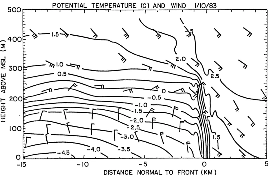
Fig. 5 presents a cross section of potential temperature with wind barbs overlayed for reference. The barb head corresponds to the aircraft position. Horizontal averaging over 1.5 km has been applied to the data to remove the smallest scale fluctuations that are evident in the plots of Figs. 3 and 4. This step was omitted, however, in the 3 km region centered on the coastal front in order to preserve the large gradients associated with the front. The temperature and wind fields outside the region shown are relatively flat and are therefore

truncated here to allow greater resolution near the front.

Two distinct air masses are evident in this cross section. The cold air is characterized by a high static stability (N

POTENTIAL TEMPERATURE (C) AND WIND

1/10/83

400

.5

2300

W~

0.5

100

-

_1..5

0

-15

-10

-5

0

5

DISTANCE NORMAL TO FRONT (KM)

Fig. 5. Cross section normal to the coastal front of potential

temperature and wind. Isotherms are drawn every 0.50 C and

-21-7-10-4 S-2 ) and weak northerly winds. A very sharp frontal interface exists up to about 300 m and separates the warm and cold air. The warm air is characterized by a weaker stability (N2 ~7-10-5 S-2) and southeasterly winds. The maximum horizontal temperature gradient is 12.9 C km-1 and extends over about 210 m distance. The maximum vertical gradient is about 30 C km-1 and occurs at about 180 m AGL well behind the surface frontal position. This is coincident with the level of greatest wind

shear.

An interesting aspect of the coastal front occuring over the water is the fact that its surface position could be observed on the ocean surface from the air. Especially from the higher elevations, the front could be seen on the surface as a dark band where there seemed to be enhanced interference amoung the surface waves. This presented a unique opportunity to observe the horizontal structure of the frontal interface. The flight observer noted that the band ran along an axis orientated between

5 and 10 degrees clockwise from the shoreline and extended at

least to the limits of visibliity. This orientation agrees quite well with that obtained from the surface analysis of Fig. 2. It was also noted that the band axis was generally straight but with

some irregualar oscillations of order 100 m in amplitude and 1 km in length imbedded in it. Therefore, provided that these observations are accurate and representative and given the fact that the aircraft data resolution is 70 m or so, then the coastal front may be regarded as essentially two-dimensional.

-22-The two-dimensionality of the coastal front allows a simplification in the study of the circulation near the front. If divergence along the coastal front may be neglected and noting that the depth of the coastal front is much less that the scale height of the atmosphere, then the incompressible continuity equation allows the circulation to be described by the stream function T=T(x,z) such that

u - (1)

w=a (2)

ax

where u and w are the front normal (positive into the warm air) and vertical wind speeds, respectivly. The stream function is then determined by integrating Eq. (1) subject to an appropriate boundary condition. (Eq. (2) could also be used, but observations of w are less reliable than those of u and the appropriate boundary condition is not obvious.) In the data analysis, u is interpolated to a grid with a 50 m vertical resolution in order to evaluate the integral of Eq. (1). The flow was assumed to be horizontal at z=O so that T(O)=O is the lower boundary condition. The. computed stream function is shown in Fig. 6. The same smoothing criterion that was applied to the potential temperature plot is used here. The convergence of

stream lines at the front again shows the narrow transition zone between the two air masses. The speed of the updraft at the front calculated using Eq. (2) is about 1.5 ms- . The apparent oscillation in the flow downstream of the updraft will be discussed later in the text.

400

300

200

100

FUNCTION

KM x (M/S)

1/10/83

-15

-10

-5

0

5

DISTANCE NORMAL

TO FRONT (KM)

Fig. 6, Stream function coastal front.

(km.m-s~1 _{) normal and relative to the}

-24-Overlaying the potential temperature field and the stream function shows that the cold air below 180 m flows weakly forward toward the front where it meets the warm, maritime air and is forced upward. Just above 180 m the air is receding from the front but is colder than the incoming maritime air. This air must represent a mixture of the two air masses, as it has the momentum of the warm air but a temperature suggesting origins in

the cold air. It is also noteworthy that the circulation extends well above 450 m even though the horizontal gradients of

temperature and wind have almost completely disappeared at that level. Unfortunately the upper extent of the circulation cannot be determined from the data.

The exchange of temperature and momentum between the two air masses can be seen more clearly by following a parcel of air that originates in the cold air near the surface. Such a parcel will closely follow the zero stream function line provided the the circulation is steady. After the parcel has ascended in the updraft and begins to recede from the front, it is warmer than it was at the surface indicating that a positive flux of heat into the cold air is occuring. The parcel has also changed the sign of its momentum indicating that either a force is acting to rearward accelerate it or that there is a flux of negative momentum into the cold air. These changes are acting to weaken the coastal front and must be balanced by a frontogenetical flux (or fluxes) in order that the coastal front maintain a steady state. One possible balancing flux is the low-level flow of cold

-25-air toward the front from the west. Certainly this flow carries the necessary positive horizontal momentum. If the flow is adiabatic, then because of the intersection between the

streamlines and isotherms near the surface, it also provides the necessary negative advection of heat. One other possible frontogenetical flux may be due to advection parallel to the front, but this possibility can not be determined here.

The above analysis suggests a mechanism for the dissipation of the coastal front. If there is insufficent flux of cold air and positive momentum into the cold air to balance that which is

swept away by the overiding warm air, then the frontal contrasts will begin to deteriorate. This could be triggered by the sudden onset of Kelvin-Helmholtz instabilities along the frontal interface. This instability has characteristics similar to breaking surface waves and its presence usually indicates a highly turbulent flow. Its presence along the frontal interface would account for the temperature and momentum changes that parcels in the cold air experience as both heat and momentum are

transported down-gradient in the turbulence.

For a fluid with stratification N2, Kelvin-Helmholtz instability may commence when the Richardson number Ri, defined

Ri= N2 RioU/az)2

falls below 0.25. An analysis of the Richardson numbers for this case using Figs. 5 and 6 interpolated to grid points shows that the region is generally stable. There are, however, pockets of

-26-potential instability above 180 m and behind the surface frontal position as well as along the forward part of the front. Further, many small regions of instability may be overlooked in this analysis because of the coarse vertical resolution of the data and the horizontal smoothing. Together, these isolated regions may be the cause of the mixing previously inferred. However, the wind shear needs to be increased by only about 25% in order to render global instability along the frontal interface. This increase is certainly possible as the warm air wind speed increases in response to the approaching cyclone. Therefore, although the easterly geostrophic wind appears necessary for coastal frontogenesis, there may be a minimun and a maximum speed that allow it to occur.

As noted earlier, the coastal front was observed first hand to be a two-dimensional feature. This property can be confirmed quantitatively by comparing the vertical wind speed from Eq. (2) with that directly measured by the aircraft. Recall that the stream function was calculated using a two-dimensional form of the continuity equation. Therefore if the calculated and observed vertical velocities are nearly identical, little mean divergence must be occuring along the front and therefore it

is two-dimensional. One problem in applying this technique to the data is that the aircraft automatically removes a 15 minute mean from the measured vertical wind so as to produce only a gust component. This should not, however, present a large discrepancy since each pass through the front took about 15 minutes.

-27-Presented in Figs. 7 (a-b) is a plot of the vertical velocities for two representative passes through the front. The high degree of correlation of the plots suggests that little divergence is occuring along the front and thus there is an overall two-dimensional structure.

One interesting feature of these plots is the presence of a sinusoidal pattern to the vertical velocity, particularly at 250 m. There is a correlation between the observed and calculated velocities within these oscillations suggesting that the phenomenon is real. These oscillations are coincident with the roll and downstream oscillations found in the stream function analysis shown earlier. They appear to be inertial gravity waves that are excited by the vertical jet and travel downstream with the mean ambient flow. The frequency for these free oscillations is just the buoyancy frequency N. The wavelength is then determined by the distance that the mean flow travels in one oscillation. For a parcel oscillating about the 250 m AGL level, the wavelength of the free modes is about 2 km. This is about 50% less than the wavelength of the observed oscillations. Therefore the observed waves may be vertically propagating gravity waves from a higher region where the stratification supports free modes of the observed wavelength. Such a region occurs at about 400 m AGL.

1.5

1.0

-0.5

w

-1.0--1.5

-

1.5-1.0:

,

0.5

Q-0P

z

--0.5

w-1.0--1.5

--

1.5

150 M AGL

-10

-5

0

DISTANCE NORMAL TO FRONT (KM)

Fig. 7a-b.

(thin

(solid

AGL.

Comparison of the aircraft measured vertical gust line) with that calculated from the stream function line) at the altitudes of a) 250 m AGL and b) 150 m

-29-Fig. 8 presents a cross section of the wind speeds parallel to the front. This plot shows that only the cold air has an appreciable parallel wind component. The shear across the front is cyclonic as Bosart et al. noted. There is an internal jet running along the front just behind the surface frontal position that lies just above the region having the strongest vertical temperature gradient. This jet may be the result of the front's attempt to achieve geostrophic balance. However a calculation of the thermal wind in the vicinity of the front shows that the observed response is only about 15% of that expected. Surface drag and vertical mixing certainly have a role in this discrepancy. The decrease in the parallel wind speed above the jet is probably a response to the strong negative advection of parallel momentum by the warm air.

Following the completion of the passes through the front the aircraft made low-level soundings at three locations between 35 and 45 km into the cold air. Compositing these sounding data with the previous cross sections shows that the coastal front maintains a vertical structure above the ground similar to that found 15 km back in the cold air. The height of the maximum in the wind shear remained near 200 m AGl and the potential isotherms remained horizontal. This type of flat downstream structure is similar to that which McCarthy found in his larger-scale cross-sections through the front.

PARR

WINDS

(M/S)

-O

-5

DISTANCE

NORMAL

0

TO FRONT

(KM)

Fig. 8. Cross section of the wind speed (ms~') parallel to the coastal front. Negative values are from the northeast.

500

400

;300

<

20

100

0--15

1/10/83

-31-The time sequence of surface synoptic maps indicates that the observations of this coastal front were made during the mature phase of frontogenesis. The front did begin to show signs of weakening about three hours after the flight as the wind in the cold air began to veer into the northeast. By 00 GMT of the llth, the front had lost much of its character in southern New England. It did however persist up to 12 hours longer along the Maine coastline.

2. Case of 15 January 1983.

The synoptic conditions that resulted in the coastal frontogenesis on this day differed little from those of the previous case. A high pressure ridge extended along the entire length of the eastern U.S. seaboard and a deep cyclone was moving into the upper Great Lakes at 00 GMT on the 15th. At the same time a new low showed signs of developing off the South Carolina coast. The pressure falls associated with this new cyclone split

the east coast ridge and formed the "V" ridge in the northeast. This allowed the geostrophic winds to become onshore. A

thickening cloud deck over New England prevented strong radiational cooling during the night, so that although coastal frontogenesis did commence by 0600 GMT of the 15th, there was not a very large initial land-sea temperature contrast.

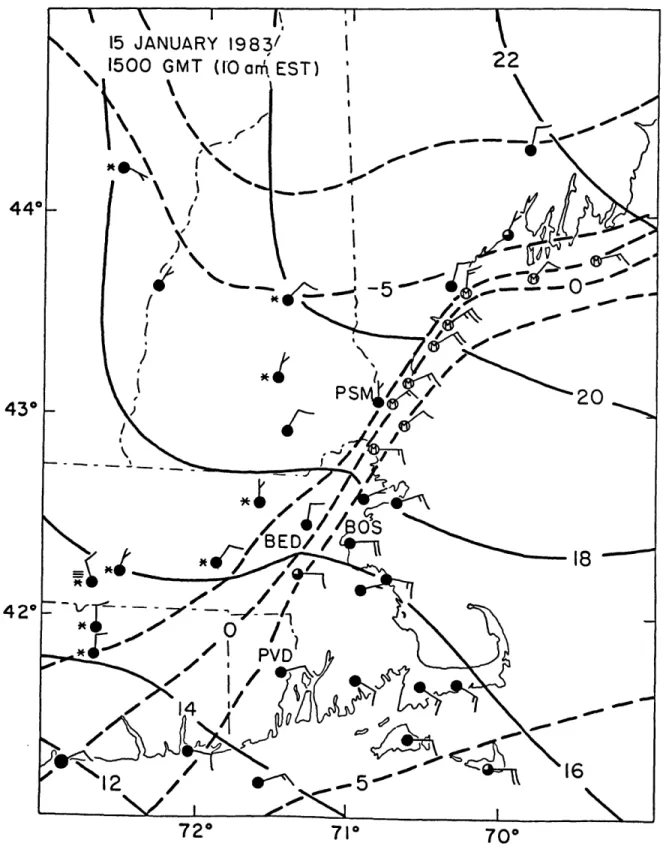
-32-The surface analysis for 1500 GMT 15 January in eastern New England is shown is Fig. 9. Comparing this analysis with the same analysis for the previous case shows that this coastal front is not as strong as in the previous case. Wind shifts appear to be less than 90 deg everywhere along the front and the isotherms are not as concentrated.

The aircraft was airborne and en route to Portsmouth by 1500 GMT. Portsmouth was again selected not only for the reasons of

the previous study, but also because light to moderate snow over much of southern and western New England prevented any low-level

research flying. The aircraft descended down to Portsmouth from a height of about 3.5 km and then made passes through the front at 75, 150, 250, 350 and 450 m AGL to 20 km on each side of the front. One pass was also made at the minimum possible elevation which varied between 15 m over water and 50 m over land. Repeat passes were made at the 75 and 250 m levels to facilitate the data analysis (see appendix). Low-level soundings were not made after the passes because of fuel constraints and deteriorating weather conditions.

Figs. 10 a-d shows plots of temperature, dew point, wind speed and wind direction for the 150 m pass (the lowest completely level pass) through the front. The front is again clearly distinguished by a sudden jump in temperature and a shift in wind direction. The contrasts across the front are not as pronounced as in the previous case with only a 2.5 C temperature

-33-4 -33-40 - -0 43*

-2

-5

43

Fig. 9.' Surface analysis in eastern New England at 1500 GMT (10 am LST) on 15 January 1983. Isobars are drawn every 2 mb and isotherms are drawn every 2.5 0C. Wind barbs are in knots. Coast guard reports are plotted with a "M".

-34-the front at this level is about 4 C and 50 deg of wind shift. Note that the wind is weaker and more northerly just to the cold side of the front. Just a few kilometers further into the cold air there appears to be a pocket of warm air, as all four plots bulge towards their warm air values.

There is a noticeable change in the variance of the dew point trace across the point coinciding with the shoreline. The vertical wind gust trace (not shown) also shows a similar change in variance and is highly correlated with the dew point trace. This suggests enhanced vertical mixing is occuring over the ocean with upward moving parcels carrying a larger moisture content. The fact that the temperature trace does not show a similar change in variance indicates that there is a relatively small vertical gradient of potential temperature.

Fig. 11 a-d shows the results of the highest pass (~ 450 m) through the coastal front. There is still a jump evident in the temperature field across the front at this height. The ratio of this jump to the jump at the lower level is considerably larger than in the previous case. The front is also marked by a weakening in the wind speed just to the cold air side of the front and a 2 ms- 1 jump in the wind speed at the front. The direction of the wind changes by nearly 30 deg over the entire data region with some turbulence-like flucuations marking the frontal position. The relatively larger temperature jump at this height as well as the frontal signature in the winds suggest that this coastal front extends deeper into the environment than was

1/15/83 150 M AGL TEMP vs. DIST -10 -5 0 5 1/15/83 150 M AGL TD

10

15

DISTANCE FROM PORTSMOUTH

20 25 20 (KM) -15 -10 -5 0 5 10 15 20 25 3601 -270' 0 LU a9

1/15/83 150 M AGL WDIR vs. DIST

180t

0 -5

DISTANCE

0 5 10 15 20

FROM PORTSMOUTH (KM) Fig. lOa-d. Plots

c) wind speed distance from

were collected

front.

of a) temperature, b) dew point temperature and d) wind direction plotted as a function of

Pease Air Force Base, Portsmoutn NH. The data during the 150 m AGL pass through the coastal

5 101 -I -101 5 -W-- 11 3 ' J a l I II A IA ,A S AI --Oak T W W w

Aj

0

1/15/83 450 M AGL WSPD vs. DIST W a. 0I .0 bi a-U, - 5 -10 -5 0 5 10 15 20 25

K4

360 1/15/83 450 MAGL WDIR vs. DIST

270

1801

-f5 -10 -5 0 5 10 15

DISTANCE FROM PORTSMOUTH

20 25

(KM) Fig. lla-d. Raw plots of a) temperature,

c) wind speed and d) wind direction distance from Pease Air Force Base, were collected during the 450 m AGL

front.

b) dew point temperature

plotted as a function of Portsmoutn NH. The data pass through the coastal -15

-37-previously seen. There is no apparent change in the variance of the dew point trace across the coastline at this height although there is a noticeable change in the variance of the vertical wind gust (not shown). Therefore there must not be a significant vertical gradient of moisture at this height.

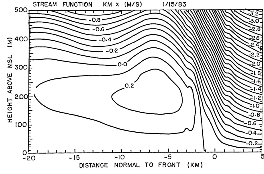
Cross-sections of the potential temperature, the stream function and parallel wind component are presented in Figs. 12, 13 and 14, respectivly. The temperature plot is expanded to include the entire 40 km region over which data were collected because there is a horizontal temperature gradient outside the immediate vicinity of the front. There are many general similarities between these plots and the equivalent ones for the previous case. There is a narrow region of tightly packed isotherms that marks the front from the ground up to about 200 m. _{The maximum horizontal gradient of temperature is 5.7 C} km-1, or about half that of the previous case. The stream function shows that the warm air flows towards the front, rises over the cold air in a narrow jet and then oscillates downstream. The cold air has a weak roll imbedded under the first wave. The parallel winds again show a low level jet just above the cold air and just above the position of maximum vertical gradient.

The front was not encountered over the ocean and therefore could not be detected visually at the surface. However a comparison between the observed and computed vertical velocities is quite good again suggesting a two dimensional structure. The maximum measured updraft is 1.3 ms-1 while the maximum calculated

POTENTIAL TEMPERATURE (C) AND WIND

1/15/83

-10

0

10

DISTANCE NORMAL TO FRONT

20

(KM)

Fig. 12. _{Cross section normal to the coastal front of potential}

temperature and wind. Isotherms are drawn every 0.50 C and

each wind barb represents a wind speed of 2.5 ms- 1_.

500

-. 400

2

300

O

100

O

t---20

KM X (M/S)

DISTANCE

NORMAL TO FRONT

(KM)

Fig. 13. Stream function

coastal front.

(km-m-s~1 ) normal and relative to the

500

400

300

1/15/83

PARR WINDS (M/S)

1/15/83

-15

-10

-5

0

DISTANCE

NORMAL

'TO

FRONT (KM)

Fig. 14. Cross section to

coastal front in ms-1.

the wind component parallel to the

Positive values are northeastward.

50

w401

300'-200

100

0--20

-41-There are some notable differences between this and the previous case. The isotherms do not become horizontal immediately behind the front but rather slope upwards away from the front. Overlaying the stream function shows that these isotherms seemingly are being advected by the flow normal to the front. However a strong downward heat flux in this region brought about by turbulence could balance the advection and allow the isotherms to remain stationary. Strong turbulence is not evident, however, as the overall flow is slightly stable to Kelvin-Helmholtz instability.

Another difference in this case is the presence of a small horizontal temperature gradient in the warm air far from the front. Recall that the previous case had only a vertical temperature gradient in this region. The vertical isotherms indicate considerable mixing is occuring. This mixing is likely due to heating from the ocean surface. Sea surface temperatures in the region were indeed from 1 to 2 C warmer than the surface air temperatures. In the absence of a heat sink for the ocean heating, the heated air will be advected toward the coastal front

and presumably cause the front to become stronger. The computed temperature advection in the warm air, about 1.25* C hr- 1, gives a frontogenesis doubling time of just less than 3 h. However a

time sequence of surface analyses after the flight shows that the front did not become more pronounced. Temperatures on both sides of the front increased and the wind on both sides slowly backed. The warming of the cold air could be due to diabatic heating. It

-42-is, however, more likely due to vertical mixing of warm air since this would also account for the changing wind direction. Therefore it appears that warm advection in the warm air and a turbulent heat flux in the cold air may be the process that allows cross frontal contrasts to remain unchanged.

Another significant difference between the present case and the previous one is the fact that light snow began to fall in the Portsmouth area during the flight. Doppler radar at MIT detected a narrow 10 dBZ band of precipitation along the coast at the surface near Portsmouth. Further south where the precipitation was more widespread, there was a 5 dBZ radar reflectivity enhancement which coincided with the coastal front position.

The flight observer noted a tendency for the snow to be found only on the cold air side of the front and that the precipitation rate increased during the flight. This observation can be quantitativly investigated using the data from the particle measuring probes. A vertical flux of particle mass can be obtained from these data using the formula

R=Z{M(D)-C(D)-V(D)}

where M is the mass of particles with diameter D, C is the concentration of the particles, and V is the particle fall speed. This flux may be transformed to a water equivalent precipitaion rate by dividing by the density of water. The summation is performed over the 15 distribution cells that the PMS probes

detect. The smallest detectable diameter is .3 mm and the upper

-43-mm. To obtain mass and fall speed from diameter, the relations (see e.g. Locatelli and Hobbs, 1974)

M=0.2-D2 and

V=2.0-D 3 1_-W(xz)

for mass M in grams, fall speed V in m-s-1 and D in cm are used. The vertical air velocity is denoted by W. The precipitation rate was calculated as a function of distance from the front for each pass through the front and then vertically averaged over all passes. This averaging was necessary because of the relatively high variance exhibited by each individual pass through the front and is justified by the relatively weak flow in the cold air. The result of this analysis is shown in Fig. 15. Note that the precipitation rate takes on a Gaussian-like horizontal distribution centered about 10.5 km to the cold air side of the front. The distribution is skewed to the cold air side of the maximum as there is little or no snow falling in the warm air. Although the mean precipitation rate is quite small, the later passes through the front measured considerable higher values.

The origin of a snowflake arriving at the position of the maximum in the precipitation rate can be calculated by

integrating backwards in time the horizontal and vertical velocities of the snowflake. This is done by assuming all particles have a uniform terminal velocity of 1.1 ms- 1 from which the calculated vertical air speed is subtracted to yield the particle fall speed everywhere. The particles are assumed to

.10

.075

E

E

.05

.025-

.00--20

-15

-10

-5

0

5

10

15

DISTANCE

NORMAL TO FRONT (km)

Fig. 15. _{Precipitaion rate computed with data from a PMS probe}

averaged over all passes through the coastal front and plotted as a function of distance normal to the front.

-45-move horizontally with the wind. The integration is carried out up to the highest aircraft pass, above which, the data from the sounding made prior to the passes are used for the horizontal winds. The vertical wind is assumed to decay linearly with height up to the warm frontal inversion (~2.3 km) from the velocity at 500 m. While this does not account for a tilt in the updraft it should not cause a serious error since the mean vertical air motion is generally much less than the particle

terminal velocity.

A few selected trajectories are shown in Fig. 16 together with the position of observed clouds, the updraft and the -2 C potential isotherm. Note that the snow generally falls down vertically after entering the cold air. This is indicative of the weak flow in this air mass. Note also that snow falling to the ground at -10.5 km passes over the position of the vertical jet at about 1.5 km above MSL. The aircraft measured a stratocumulus cloud base at about 1.1 km which is almost exactly the lifted condensation level of the surface warm air. The top of the clouds was at about 1.8 km. Therefore snow falling at the point of the observed maximum precipitation rate originated from a position within clouds and above the vertical jet. Since the MIT radar detected no echoes near Portsmouth above 2 km, the observed snow must have grown within the stratocumulus clouds. Therefore it seems likely that the coastal front is leading directly to the enhancement of the precipitation at the surface.

2.0

1.5

-20

-15

-10

-5

0

5

DISTANCE NORMAL TO FRONT (KM)

Fig. 16. Computed snowflake trajectories shown schematicaly with

the position of the observed clouds, the -2* C potential

-47-One aspect of the precipitation enhancement associated with the coastal front is that differential evaporative cooling can occur across the front. With heavier precipitation and lower dew point temperatures, the cold air will be cooled to a greater degree than the warm air. Therefore this evaporative cooling could offset any turbulent diffusion of the front, sustaining or even enhancing the coastal front.

The coastal front persisted for about 12 hours after the conclusion of the flight, lasting during most of what became a fairly intense storm throughout New England. The coastal front played a major role in determining the distrubution of the total snow accumulation. Boston, for example, remained generally on

the warm side of the coastal front and primarly received a mix of rain and wet snow. The recorded snow accumulation was less than

10 cm. On the other hand, regions less than 30 km to the north-west that remained in the cold air, received up to 60 cm of snow.

-48-CHAPTER III

THE DENSITY CURRENT ANALOGY

A density current is the flow that results when one fluid undercuts another less dense fluid. From the analysis presented in the last section, the coastal front seems to resemble this type of flow. In fact, Ballentine noted that the flows produced in his numerical simulation of the coastal front behaved similarly to a density current. Later Passarelli and Braham

(1981) showed that Great Lake snow squalls were often intimately related to a density current-like land breeze and speculated that a similar effect might be occurring for the coastal front. Therefore, a summary of the properties of a density current and a comparison to the observed properties of the coastal front is warranted here.

If the wall separating two fluids of different density is suddenly removed, the denser of the fluids accelerates horizontally and undercuts the lighter fluid. The acceleration is the result of a horizontal pressure gradient that arises because of different hydrostatic pressures in the two fluids. The denser fluid continues to accelerate until a dynamic pressure due to the convergence of mass at the interface balances the pressure gradient. The resulting steady flow is called a density (or sometimes a gravity) current. The current moves under the

-49-ambient fluid at a constant phase speed. In the presence of viscosity, this phase speed may be somwhat reduced. Long after the density current is established, the boundary between the two fluids becomes flat except near the leading edge of the current.

The most extensive analytical treatment of the inviscid density current was made by Benjamin (1969). In the case of a density current imbedded in an infinitly deep fluid, he concluded that the speed of the density current through the ambient fluid is given by

V=k/(gH(P₂-P1)/P1 )

where pi is the density of the ambient fluid, P2 is the density of the invading fluid with depth H, and g is the gravitational acceleration. The constant of proportionality k is /2. Benjamin further found the structure of the invading fluid to consist of a head wave that rises somewhat higher than the downstream mean depth H. He also showed that wave breaking must occur on the head leading to considerable turbulence downstream.

If viscosity, heating or stratification is included in the analysis, the density current problem becomes considerably more difficult and therefore most of what is known about these types of density currents has been learned in laboratory tank experiments similar to those described above. Kleugan (1958, 1959), Middleton (1966) and Simpson (1969) all carried out this type of experiment usually using segregated saline water with densities differing by a few percent. The results generally

-50-indicate that within a wide range of Reynolds numbers, including those most often found in the atmosphere, density currents exhibit behavior similar to that described by Benjamin. Fig. 17 shows a schematic diagram of a typical laboratory density current constructed from the work of Kleugan, Middleton and Simpson. Major differences between the theoretical and laboratory currents include a slightly lower value of k and varying degrees of turbulence on the back side of the head. The laboratory currents were also found to have a protruding nose of the denser fluid at the leading edge of the current. This arises because surface friction retards the advancement of the dense fluid near the lower boundary. The maximum height of the head wave is often found to be about twice the downstream fluid depth, but this depends upon the degree of breaking on the head. Middleton noted that the individuality of different density currents is often apparent in the shape of the head. He noted that the elongation and height of the head is dependent upon the Reynolds nunber. For high Reynolds number flows, such as in the atmosphere, density current heads will exhibit a characteristic aspect ratio

(= head height/head length) significantly smaller than is usually found in saline solution laboratory experiments.

Some naturally-occuring flows that behave similarly to a density current are saline intrusion into an estuary, turbidity (or mud) flows along a lake bottom and, to some degree, avalanches. In the atmosphere where sharp density contrasts are most often brought about by sharp virtual temperature contrasts,

Fig. 17. Schematic ,diagram

current produced using two

of a typical laboratory density

-52-many density-current-like flows have been found. Berson (1958) showed that the leading edge of a cold front has a density current structure. Simpson found a similar structure in sea breezes and haboobs. Both Charba (1974) and Goldman and Sloss (1969) made sucessful analogies between analyzed thunderstorm outflows and a theoretical density current.

A visual comparison between Fig. 17 and either Fig. 6 or 13 shows that the coastal front indeed shares many structural similarities with a classical density current. The characteristic aspect ratio of the coastal front head is considerably different than that shown in Fig. 17, as should be expected from Middleton's work. Nonetheless, there is considerable similarity in the basic structure of the model density current and that of the coastal front. There is a head wave in the coastal front that rises about 25% above the mean downstream depth. There is a roll in the circulation within the head wave on both flows as well as condsiderable downstream mixing. Absent from the coastal front structure is a protruding nose. Middleton found, however, that the height of the nose may be as low as .07-H or about 15 m for the coastal front and thus too low to be detected by aircraft. Further, because the cold air mass in both coastal front cases is nearly stationary with respect to the surface, frictional drag of the cold air will be weak and therefore a nose may not exist.

-53-Benjamin's phase speed equation may be appled directly to the coastal front analysis provided density is replaced by virtual potential temperature, i.e.

P2~P 1=0V2-6vi

P1 0v₁

which is derived using the equation of state for moist air. If in applying this to the front, H is taken to be 500 m, then ev₂-evi is the average virtual temperature difference in the layer up to 500m. From the potential temperature analysis, this number evidently accounts for most of the temperature difference across the front. Since the velocity of the front and the mean air speed normal to the front are known independently (see appendix), the proportionality constant k may be determined. The results of this calculation for the two cases presented are shown in Table 1. It can be seen that the values of 1.03 and 1.10 for k in both cases are less than the V2 Benjaman found for an inviscid density current. They are, however, within the range of k's found for other density-current-like atmospheric flows. For

instance, Charba found k=l.25 in a thunderstorm outflow and Simpson found k less than one for sea breezes. Therefore it seems that the coastal front may well be modeled both in structure and dynamics by a typical two-fluid density current model.

-54-Table. 1. Application of Benjamin's eq. to the coastal front. case Aev gH-AOv/0vi observed V mean wind total obs. V k Jan 10 2.92*C 7.25 ms- 1.50 ms-1 6.0 ms-1 7.5 ms-' 1.03 Jan 15 2.950C 7.28 ms-1 1.35 ms-I 6.7 ms-I 8.05 ms-I 1.11

-55-CHAPTER IV

SUMMARY AND DISCUSSION

The vertical structure of two New England coastal fronts was observed by aircraft along the New Hampshire coast. It is found to consist of two distinct air masses that are separated by a narrow transition zone. Although most of the front's horizontal signature lies below about 300 m, some features, especially the circulation field, extend to at least 500 m. The flow near the front has been shown to be basically two-dimensional. A vertical jet of about 1.5 ms- 1 characterizes the coastal front and seems to be directly responsible for an observed precipitation enhancement downstream. There is also evidence of considerable mixing along the frontal interface although both cases did not, in general, support Kelvin-Helmholtz instabilities. The coastal front is also shown to be similar to a two-fluid density current. If the primary balance of forces for the steady coastal front is that which governs a density current, then the favored positioning of the coastal front that Bosart et al. noted may be

accounted for. Recall that the coastal front is most often found along the coast in New Hampshire and Maine, but well inland in Massachusetts and southward. This position is approximately equivalent to where the flat coastal plain meets the first hills of the Appalachians Mountains. If these mountains act as a dam to any westward movement of the cold air, then because of mass conservation, the depth of the cold air and thus the surface gradient of hydrostatic pressure, must vary as the inverse of the