Accepted
Article
This article has been accepted for publication and undergone full peer review but has not
been through the copyediting, typesetting, pagination and proofreading process, which may
lead to differences between this version and the Version of Record. Please cite this article as
doi: 10.1002/ecm.01296
MR. MARC-ANDRÉ LEMAY (Orcid ID : 0000-0003-2484-8447)
Article type : Article
Spatially explicit modelling and prediction of shrub cover increase near Umiujaq, Nunavik
Marc-André Lemay1,2, Laurence Provencher-Nolet2,3, Monique Bernier2,3, Esther Lévesque2,4, Stéphane Boudreau1,2,5
1 Département de biologie, Université Laval, 1045 Avenue de la Médecine, Québec, QC, Canada G1V 0A6
2 Centre d’études nordiques, Université Laval, 2405 Avenue de la Terrasse, Québec, QC, Canada G1V 0A6
3 Institut national de la recherche scientifique – Centre Eau Terre Environnement, 490 Rue de la Couronne, Québec, QC, Canada G1K 9A9
4 Département des Sciences de l’environnement, Université du Québec à Trois-Rivières, 3351 Boulevard des Forges, CP 500, Trois-Rivières, QC, Canada G9A 5H7
Running Head : Spatial modelling of shrubification
Manuscript received 28 June 2017 ; revised 11 December 2017 ; accepted 16 January 2018. Corresponding Editor : Daniel B. Metcalfe
5
Accepted
Article
Abstract
A circumpolar increase in shrub growth and cover has been underway in Arctic and subarctic ecosystems for the last few decades, but there is considerable spatial heterogeneity in this
shrubification process. Although topography, hydrology and edaphic factors are known to influence shrubification patterns, a better understanding of the landscape-scale factors driving this phenomenon is needed to accurately predict its impacts on ecosystem function. In this study, we generated land cover change models in order to identify variables driving shrub cover increase near Umiujaq
(Québec, Canada). Using land cover maps from 1990/1994 and 2010, we modelled observed changes using two contrasting conceptual approaches: binomial modelling of transitions to shrub dominance and multinomial modelling of all land cover transitions. Models were used to generate spatially explicit predictions of transition to shrub dominance in the near future as well as long-term
predictions of the abundance of different land cover types. Model predictions were validated using both field data and current Landsat-derived trends of NDVI increase in the region in order to assess their consistency with observed patterns of change. We found that both variables related to
topography and to vegetation were useful in modelling land cover changes occurring near Umiujaq. Shrubs tended to preferentially colonize low-elevation areas and moderate slopes, while their cover was more likely to increase in the vicinity of existing shrub patches. Deterministic realizations of the spatially explicit models of land cover change had a good predictive capability, although they performed better at predicting the proportion of different cover types than at predicting the precise location of the changes. Binomial models performed as well as multinomial models, indicating that neglecting land cover changes other than shrubification does not result in decreased prediction accuracy. The predicted probabilities of shrub increase in the region were consistent with patterns of change inferred from field data, but only partly supported by recent local increases in NDVI. Our findings increase the current understanding of the factors driving shrubification, while warranting further research on its impacts on ecosystem function and on the link between land cover changes and shifts in remotely sensed vegetation indices.
Accepted
Article
Key words
Arctic ecology; ecological modelling; land cover change; Landsat; landscape ecology; NDVI; Northern Québec; shrubification; remote sensing; vegetation change model
Introduction
Arctic and subarctic ecosystems are deeply altered by climate change and will likely be more impacted by temperature increases than will be temperate ecosystems due to Arctic amplification (Serreze and Barry 2011, IPCC 2013). In recent decades, obvious changes observed in high-latitude environments include an increase in temperatures, a decrease in summer sea ice cover, and permafrost thaw (Hinzman et al. 2013). One of the most important changes in terrestrial ecosystems is a greening of the tundra, inferred from an increase in normalized difference vegetation index (NDVI) since the 1980s (Bhatt et al. 2013, Ju and Masek 2016). This greening trend has been repeatedly documented using remote sensing data spanning resolutions from 8 km AVHRR data (e.g. Goetz et al. 2005, Jia et al. 2009) to 30 m Landsat data (e.g. Fraser et al. 2011, McManus et al. 2012, Fraser et al. 2014), and although browning (i.e. a decrease in NDVI) has been observed in some areas, greening remains the dominant trend in subarctic regions (Ju and Masek 2016).
Although only successfully calibrated in a few locations, several studies have attributed increases in tundra ecosystem NDVI to an increase in shrub cover and size in response to climate change, a phenomenon termed shrubification (Forbes et al. 2010, Myers-Smith et al. 2011a, McManus et al. 2012). Repeat aerial photography yields evidence for a sharp increase in shrub cover in Alaska (Sturm et al. 2001, Tape et al. 2006), Northwestern Canada (Lantz et al. 2013, Fraser et al. 2014), Subarctic Québec (Ropars and Boudreau 2012, Tremblay et al. 2012, Provencher-Nolet et al. 2014) and Siberia (Frost and Epstein 2014), indicating that this phenomenon might be circumpolar in scale. The link between warmer temperatures and shrub cover is supported by experimental warming studies that found higher shrub cover and/or height in response to increased temperature (Chapin et al. 1995, Walker et al. 2006, Elmendorf et al. 2012a). Dendroclimatic analyses also support a positive effect of warmer temperatures on shrub growth, reinforcing the idea that the increase in global temperatures
Accepted
Article
might favour this plant functional group (Forbes et al. 2010, Hallinger et al. 2010, Blok et al. 2011a, Ropars et al. 2015a, Ropars et al. 2017). Moreover, the growth structure of some shrub species is thought to allow them to benefit more from increasing temperatures than other plants (e.g. Betula
nana L.; Bret-Harte et al. 2001).
A significant increase in shrub cover and height could deeply alter the structure and function of tundra ecosystems. Shrubification might lead to a reduced overall albedo in terrestrial Arctic regions because of the low albedo of shrubs, effectively resulting in a positive feedback to climate change (Chapin et al. 2005, Sturm et al. 2005a, Bonfils et al. 2012). Shrubs also affect patterns of snow deposition and accumulation as well as snowmelt by respectively trapping snow (Sturm et al. 2005b) and accelerating thaw in spring because of the low albedo of protruding branches (Marsh et al. 2010). By maintaining a thicker insulating snow cover, shrubs also lead to warmer winter soil temperature under erect shrub cover and may thus contribute to an increase in active layer depth and permafrost degradation (Sturm et al. 2005b, Lantz et al. 2013, Myers-Smith and Hik 2013, Paradis et al. 2016). This should
effectively lead to another positive feedback loop by which this deeper active layer favours nutrient mineralisation, thus increasing their availability for shrub growth (Sturm et al. 2005b, DeMarco et al. 2011; but see Myers-Smith and Hik 2013). An increase in shrub cover could also have seasonal impacts on the diet of large herbivores such as caribou, which rely heavily on lichens during winter to meet their energy requirements (Sturm et al. 2005b, Joly et al. 2007).
Although observed throughout most of the circumpolar region, the rate and extent of shrubification are highly heterogeneous in space. At larger scales, shrub cover increase has been found to occur preferably in the warmer and wetter Low Arctic as compared to the cold and dry High Arctic (Elmendorf et al. 2012b, Myers-Smith et al. 2015). The rate of shrub cover increase is also known to vary at a regional scale, depending on edaphic, topographic or historical conditions (Tape et al. 2012, Tremblay et al. 2012, Fraser et al. 2014, Ropars et al. 2015b). For example, Ropars and Boudreau (2012) found that shrub cover increase occurred preferably on sandy terraces as opposed to hilltops, while Tape et al. (2006) observed that hill slopes and valley bottoms favoured a greater increase in
Accepted
Article
shrub cover. Recent research showed that sites offering greater nutrient and water availability favour shrub growth (Naito and Cairns 2011, Tape et al. 2012, Cameron and Lantz 2016, Curasi et al. 2016) and that shrub growth sensitivity to climate is higher in wetter regions (Myers-Smith et al. 2015).
A better understanding of the landscape-scale factors driving shrub growth and recruitment is required in order to predict shrubification patterns and impacts on the dynamics of high-latitude ecosystems in the near future. This phenomenon currently occurring in high-latitude regions could be appropriately modeled using a land cover change modelling approach. Several studies made use of such models in order to gain insight into the factors underlying land cover changes and generate predictions to inform land management. For example, land cover change models were used to predict directional changes due to either land abandonment (e.g. Rutherford et al. 2007, Gellrich et al. 2007, Prishchepov et al. 2013) or urbanisation (e.g. Araya and Cabral 2010). Spatially explicit models of land cover change often model the outcome of change as a function of landscape characteristics using binomial (e.g. Pueyo and Beguería 2007), ordinal (e.g. Rutherford et al. 2007) or multinomial (e.g. Augustin et al. 2001) logistic regression.
In the region of Umiujaq, in Nunavik (Subarctic Québec), directional changes to shrub dominance have already been documented in the Tasiapik valley using aerial photography (Provencher-Nolet et al. 2014) and satellite data (Beck et al. 2015). In the present study, we implement a modelling approach meant to identify landscape-scale factors promoting shrubification in subarctic
environments using data from Umiujaq. Unlike most land cover change studies, which rely entirely on satellite data or aerial photography, we have carried observations in the field in order to assess how our model predictions were supported. We also validated our models with independent Landsat-derived NDVI data in order to assess whether current trends in NDVI change are consistent with model predictions. Our aim was to answer the following four questions: 1) What are the landscape-scale variables driving shrubification near Umiujaq? 2) How is vegetation expected to change in the area in the future, based on how it changed in the past? 3) How are the results of the predictions supported by observations in the field? 4) How are the results of the predictions supported by current trends in Landsat-derived NDVI data?
Accepted
Article
Methods
Study area
Our study area is located near the community of Umiujaq, Nunavik (Subarctic Québec, Canada), south of the latitudinal treeline (Fig. 1). Mean annual temperatures of -3.0°C have been recorded in Umiujaq between 2002 and 2013 (CEN 2014). In Whapmagoostui-Kuujjuarapik, located
approximately 160 km to the south-west, data spanning a longer interval show a mean yearly temperature of -4.2°C between 1958 and 1989 and -3.0°C between 1990 and 2015 (Environment Canada 2016). The yearly data for both locations over the period 2002-2013 are highly correlated (r = 0.998), mean temperatures being on average 0.5°C lower in Umiujaq (Appendix S1: Fig. S1).
Previous studies have documented an increase in shrub cover near Umiujaq over the last 20 years (Provencher-Nolet et al. 2014, Beck et al. 2015). The most common erect shrub species in the area are
Betula glandulosa Michx. (dwarf birch), Alnus viridis (Chaix) D.C. ssp. crispa (Aiton) Turrill
(mountain alder) as well as several Salix (willow) species (most commonly S. planifolia Pursh and S.
glauca L.). Betula glandulosa is commonly recognized as the main species contributing to shrub
expansion in Nunavik (Ropars and Boudreau 2012, Tremblay et al. 2012, Ropars et al. 2015a), although other erect shrub species may be involved as well. Picea mariana (Mill.) B.S.P. (black spruce) is the only tree species commonly found in the region.
Two different areas were considered for the purpose of our study: the Tasiapik valley (~5.33 km2), hereafter referred to as "the valley", and the coastal area south of the village (~1.98 km2; Fig. 1), hereafter referred to as "the coast". These areas were chosen because they represent two contrasting landscapes (coastal and inland) for which a long tradition of research has resulted in abundant data and a good understanding of their ecological dynamics. Elevation in the valley study area ranges from 0 on the shore of the Tasiujaq Lake (formerly known as the Richmond Gulf or Lac
Guillaume-Delisle) to about 200 m, although most of the area of interest lies below 150 m a.s.l. Shrubs dominate the vegetation of the valley (59.9% of the area as of 2010), while lichens and herbaceous vegetation are dominant on scattered permafrost mounds. Small, relatively uncommon herbaceous patches are
Accepted
Article
also distributed over the area, mainly around the numerous water ponds found in the valley. The center of the valley, largely sheltered from the wind, is dominated by black spruce. The height of erect shrubs in the valley ranges from ca. 10 cm on the lichen-dominated plateau overlooking the valley to > 2 m (mostly Alnus and Salix stands) closer to the Tasiujaq Lake.
The coast study area spans about 2 km along the shore of the Hudson Bay and 1 km inland. Shrubs are also the main land cover type on the coast (35.9% of dominance as of 2010), whereas large patches of herbaceous (more common than in the valley) and lichen vegetation are scattered in the landscape. In the southern part of the coast, land cover is characterized by sparsely vegetated rock outcrops. Almost no trees are found on the coast, as conditions are colder and windier than in the valley. Erect shrub height ranges from ca. 30 cm to > 2 m (mostly Alnus and Salix stands), but is on average lower than in the valley. Both the valley and the coast are disturbed to some extent by human activities (e.g. by road construction or ATV trails), but human disturbance is more important on the coast as this area is located closer to the community.
Land cover classification
Land cover classification of the valley has been carried out and described by Provencher-Nolet et al. (2014), who classified 30-cm resolution 1994 and 2010 aerial photographs into six different land cover classes (Table 1; Appendix S1: Fig. S2a) using an object-based supervised classification method with the eCognition software (Definiens AG, Germany). For the purpose of our study, the coast vegetation was similarly classified using aerial photography from 1990 and 2010 (Appendix S1: Fig. S2b). We used aerial photos from 1990 instead of 1994 for the coast because the quality of the existing 1994 aerial photography of the coast did not lend itself for land cover classification. Compared to the Tasiapik valley, a “sand” cover class was added to the coast classification whereas the “spruce” cover class was removed as almost no trees are found on the coastline (Table 1). Sand cover on the coast comprises both the beach running along the shore and the sand dunes protruding farther from the Hudson Bay. Details regarding the validation of the land cover maps can be found in supplementary material.
Accepted
Article
Topographic variables
A 1 m-resolution digital elevation model (DEM) was derived from a 2010 airborne LiDAR survey using the blast2dem function of LAStools (rapidlasso GmbH, Germany). This DEM was resampled to a 5 m-resolution raster from which we derived four different topographic variables to be used in land cover change modelling. Elevation was obtained directly from the DEM. We chose to include elevation in our models because of its important effects on factors such as temperature and wind exposure. Slope and aspect were computed using the algorithm of Zevenbergen and Thorne (1987), as implemented in QGIS 2.8.1 (QGIS Development Team 2015). Aspect was not used as a predictive variable in itself but rather transformed using the method described by Beers et al. (1966), which allows it to be represented on a continuous scale (here, SW = 0 and NE = 2). Slope should influence soil moisture and mineral content, while both slope and aspect have an influence on
photosynthetically active radiation exposure. The topographic wetness index (TWI), a measure of the potential moisture of the soil based on terrain characteristics, was computed using SAGA algorithms (Conrad et al. 2015) in QGIS. We included this variable in our analysis because shrubification is known to be favoured by higher soil moisture content. In fact, shrubification was found to be related to TWI in a previous study (Naito and Cairns 2011).
Vegetation-related spatial variables
A series of six vegetation-related spatial variables was derived from the land cover maps. All variables were obtained for a 5 m-resolution raster (grid) after rasterizing the polygon-based land cover maps. Rasterization was carried out using the 5 m-resolution DEM to ensure that all variables were aligned. A small part (~ 5%) of the land cover map of the valley was not covered by the DEM and was thus not retained for land cover change analysis. Roads and other disturbed areas were similarly masked and excluded from further analysis. Resampling to a resolution of 5 m resulted in similar proportions of the different land cover types and land cover changes as the original
classification. We decided to carry the modelling on 5 m pixels, as this was the highest resolution at which we deemed changes to be reliably observed over a timespan of approximately 20 years, given the quality and resolution of our data. We have also carried out a sensitivity analysis by conducting
Accepted
Article
analyses at lower resolutions of 15 and 30 m and found results to be largely similar to those obtained from 5-m resolution data (see Supplementary material for details).
Vegetation, a six-class categorical variable identifying the dominant land cover type in a given cell,
was itself used as a predictor variable. We expected this variable to be the main predictor of land cover changes, as all land cover types are not equally likely to be colonized by shrubs. Edge is a binary variable indicating whether a cell is located at the edge of the land cover patch it is part of (i.e. whether it "touches" other land cover types). Cells located at edges should be more likely to switch land cover types because of vegetative propagation and/or because their environmental conditions might suit other vegetation types. Shrub edge, similarly, is a binary variable indicating whether there is at least one shrub-dominated cell in the immediate (8-cell) neighborhood of a cell; such cells should have a higher likelihood to become shrub-dominated in the future. Neighborhood was defined as the number of cells of the same vegetation type as the focal cell in a 24-cell Moore neighborhood (5x5 pixel square). This was treated as a numeric variable with integer values ranging from 0 to 24 (see also Augustin et al. 2001). We expected cells with lower neighborhood values to be more likely to change as these are more exposed to other land cover types. Considering the 24 neighboring cells instead of the 8 immediately surrounding cells took into account the broader context in which cells were located and thus provided a more detailed description of the configuration of vegetation than
edge, while also ensuring more inter-cell variability. Edge ratio is a continuous numeric variable
computed by dividing the number of border cells in a patch by the total number of cells in that vegetation patch; edge ratio values are therefore identical for all cells in a given patch (see also Augustin et al. 2001). Higher edge ratio values represent thin and/or irregularly shaped patches, whereas lower edge ratio values are representative of large, more or less circular patches that should be less likely to change since they are less exposed to other land cover types. Surrounding is a variable identifying the dominant cover type in a 24-cell Moore neighborhood surrounding the focal cell. Were there ties between different cover types in the 24-cell neighborhood, larger square neighborhoods were used around the focal cell until ties could be broken. We expected cells to be more likely to change to or stay in the land cover type that is the most common one in their
Accepted
Article
neighborhood. Values for variables that depended on surrounding cells (edge, shrub edge,
neighborhood, surrounding) were set to missing if any of the cells implied in the computation had
missing values in order to account for edge effects.
Statistical modelling of vegetation change for the 1990/1994 to 2010 period
In order to compare different conceptual representations of the land cover changes occurring in our study area, we tested two contrasting statistical modelling approaches: multinomial and binomial logit modelling (Fig. 2).
We used multinomial logit models to represent a process of vegetation change in which transitions from and to any land cover type occur (see also Augustin et al. 2001, Rutherford et al. 2007). In order to represent all vegetation changes between any of the six land cover types (36 transitions in total, including same-state transitions), we fit multinomial logit models using the dominant vegetation in 2010 as a response variable and the 1990/1994 values of explanatory variables. A multinomial logit model allows calculating the transition probabilities to every vegetation type given the values of different predictor variables.
We used binomial models to represent the conceptual assumption that the only transitions occurring are those that lead to shrub dominance (see Pueyo and Beguería 2007 for a similar approach). To fit these models, the 2010 vegetation variable was converted to a binary variable (shrub-dominated or not). This assumption neglects other vegetation changes that do happen in the ecosystem (including transitions from shrubs to other land cover types), but might be a better representation of reality given the important shift to shrub-dominated vegetation currently observed. We could make this assumption because transitions from shrub cover to other cover types were relatively rare compared to other transitions, with only ~14% of shrub pixels transitioning to other land cover types (8 of these 14% being transitions to spruce cover that are likely due to misclassification; see Supplementary material). Binomial models are also simpler to parameterize and interpret. The model prediction output
shrub-Accepted
Article
dominated at a later time. Since this conceptual model did not consider transitions from shrub dominance to any other cover type, we only considered cells that were not shrub-dominated at time 1 in the analysis. Cells that were already shrub-dominated were thus assigned a de facto probability of transition to shrub cover of 1.
Analyzing such rasterized spatial data as if pixels were independent from one another would result in a substantial over-estimation of the actual sample size available for analysis, as neighboring pixels are spatially autocorrelated. In order to avoid this artificial inflation of sample size and avoid detecting spurious effects, we opted for an approach similar to that of Rutherford et al. (2007) and Müller and Zeller (2002) and took a regular sample of pixels 35 m apart (about 2% of the total number of pixels in the dataset) in both the x and y directions from the top left pixel of each raster. Regular sampling (as opposed to random sampling) ensures both repeatability of the analysis and uniform sampling of the whole dataset. Our sampling resulted in a total of 3,671 pixels retained for the valley and 1,461 pixels retained for the coast in multinomial modelling. As shrub-dominated pixels were not
considered in binomial modelling, only 1,946 of these pixels were kept for the valley and 1,174 pixels for the coast.
We adopted a multimodel inference framework (Anderson 2008) in order to identify the most likely statistical model or set of statistical models for each of the four modelling situations (multinomial and binomial logit modelling for both the coast and the valley). As testing all possible model
combinations of the 10 explanatory variables would have resulted in 1024 models (ignoring
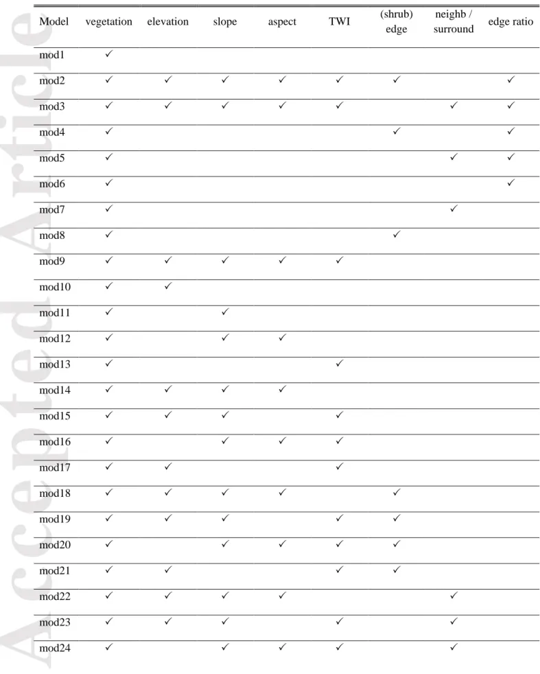
interaction and polynomial terms), we had to narrow the set of models. Notable a priori model design decisions that we made in that sense were: (1) vegetation was included in all models, as current vegetation plays an obvious role in determining vegetation at a later time; (2) shrub edge and
neighborhood were used only in binomial models, whereas edge and surrounding were used only in
multinomial models, as these variables were deemed more relevant to the conceptual processes represented by these modelling approaches (because binomial models focus on transition to shrub dominance whereas multinomial models consider all transitions); (3) shrub edge and neighborhood
Accepted
Article
were never included in the same (binomial) model as they both imply some representation of the surrounding cells, as were edge and surrounding for multinomial models; (4) whenever (transformed)
aspect was included in a model, slope as well as the interaction between slope and aspect were also
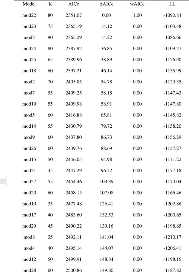
included as the effect of aspect is expected to be stronger on steeper slopes; (5) whenever slope was included in a model, we also added a quadratic term for slope since we expected shrubification probabilities to increase on intermediate slopes and decline on very steep slopes based on the current understanding of the phenomenon (Tape et al. 2006, Tremblay et al. 2012). The sets thus differed whether they were used in multinomial or binomial modelling, but they were identical for the valley and the coast. These considerations resulted in 29 binomial and 29 multinomial models representing a set of different conceptual hypotheses about the vegetation change process occurring near Umiujaq (Table 2). Models were parameterized by using the state of vegetation in 2010 as a dependent variable and vegetation characteristics in 1990/1994 in the computation of vegetation-related explanatory variables. Topography in 1990/1994 was assumed not to be significantly different from that of 2010, so we used the 2010 LiDAR-derived terrain data to parameterize the models. Although periglacial processes are known to influence topography in the study areas (Beck et al. 2015), these changes in topography are unlikely to be important enough to drive land cover changes over the temporal and spatial scales considered. Moreover, large-scale topographic changes such as thaw slumps or frost boils have not been observed in the study area. Models in each set were ranked according to their AICc values, and model AICc weights were computed to compare the models to each other. We computed 95% confidence intervals with model-averaged mean values and unconditional variances to assess the importance and effect sizes of model terms included in the 95% confidence model set. Throughout the study, model averaging was used if the best model in the set had an AICc weight < 0.90; otherwise, the single best model was used for statistical inference and predictions.
Spatially explicit modelling and prediction of vegetation change over the next decades
Model predictions were generated for the whole dataset (173,764 pixels for the valley and 69,044 pixels for the coast) using model averaging (when applicable), i.e. model predictions were computed using all models by weighting according to model probabilities (i.e. AICc weights; Anderson 2008).
Accepted
Article
The actual predictions generated from either the binomial or multinomial models can be visualized as probability maps of transition to shrub dominance (for binomial models) or to any land cover type (for multinomial models), but they do not generate a predicted vegetation map directly. Following Carmel et al. (2001), we tested both a deterministic and a stochastic way of translating the statistical model predictions into spatially explicit predictions of vegetation at a later time. For binomial logit models, stochastic modelling was implemented by setting the vegetation class of a cell at a later time to shrub dominance with a probability equal to the value predicted for that cell, whereas deterministic
modelling was implemented by setting all cells with a probability > 0.5 to shrub dominance. For multinomial models, stochastic modelling was implemented by setting the land cover of each cell to any of the six cover types depending on the multinomial distribution calculated for that cell based on the model (as in a Markov chain), whereas deterministic modelling was implemented by setting the land cover at a later time to the vegetation type for which the transition probability was highest.
Our analysis yielded eight different predicted map types (all combinations of coast or valley, multinomial or binomial, and stochastic or deterministic). The performance of these predictions was assessed by testing how well the 2010 land cover could be predicted from the 1990/1994 data. We computed the quantity and allocation disagreement and the standard kappa coefficient for every spatially explicit prediction, as described in Pontius and Millones (2011). Quantity and allocation disagreement values split total disagreement (1 - overall accuracy) into two components, respectively the disagreement due to errors in the number of pixels in different classes, and the disagreement due to errors in location of the pixels. Mean and standard deviation of disagreement metrics and kappa values for stochastic realizations of the model predictions were obtained from 100 independent runs. For binomial deterministic models, we also calculated the area under the curve (AUC) of the receiver operating characteristic (ROC) plots of shrub cover prediction by varying the threshold value
necessary for a cell to undergo transition to shrub dominance from 0 to 1.
Spatially explicit predictions of future land cover were generated using the 2010 data for both the valley and the coast. These predictions are valid for 2026 for the valley and 2030 for the coast because our models describe vegetation changes occurring over time steps of 16 and 20 years, respectively, for
Accepted
Article
the valley and the coast. We generated shrubification probability maps for 2026 and 2030 as well as long-term (~100 years) predictions of the proportions of land in each cover class. We do not expect our models to be accurate up to that time, but we were interested in the long-term behaviour of each of the models and how they might be impacted by model design decisions. Vegetation-related variables were dynamically updated at each time step to account for the new configuration of the vegetation that resulted from the changes, although we ignored neighboring missing values (contrary to what was done for model parameterization) as this would have resulted in a substantial loss of data at every time step due to the propagation of missing data at the edges.
Field-based model corroboration
We carried observations in the field in order to validate the 2010 land cover maps and to assess how our model predictions were supported. Field observations were aimed at identifying which sites had the potential to transition to shrub dominance in the near future according to their present shrub cover and location at the margin of an erect shrub stand. In August 2015, we surveyed 150 points in the valley and on the coast, for a total of 300 sampling points. Points were randomly selected using a stratified sampling protocol so as to survey points from the whole range of land cover types, elevation and slope conditions found in the area. No point was surveyed in spruce-dominated stands in 2015 because we deemed unlikely, based both on previous analysis by Provencher-Nolet et al. (2014) and the life-history traits of the various species, that spruce stands would be replaced by shrubs in the absence of disturbance. Some points (n = 19) in the valley had to be randomly relocated during fieldwork because access to these sites proved to be difficult. Field surveys consisted of a series of measurements and observations taken on both a 3 x 3 m and a 9 x 9 m quadrat centered on the survey point, which was positioned using a Garmin etrex30 GPS device. For each quadrat, we assessed the percentage cover of each of the 6 land cover classes found in the zone according to an eight-class system (0%, 1-10%, 11-25%, 26-50%, 51-75%, 76-90%, 91-99%, 100%). We also noted whether the quadrat was located at the margin of an erect shrub stand (yes/no). The 3 x 3 m quadrats were used to validate the land cover maps, whereas 9 x 9 m quadrats were used to assess the support for spatially explicit model predictions.
Accepted
Article
At the end of July 2016, we conducted additional field surveys in order to refine the validation of the coast and valley vegetation maps. Thirty-six (36) surveys as described above were conducted on the Umiujaq coast in order to increase the sample size for vegetation types that were underrepresented in 2015; these surveys were also included in the assessment of the accuracy of spatial predictions (described below). In the valley, 20 spruce-dominated stands were surveyed in 2016 since this vegetation class had not been surveyed in 2015; the objective of these spruce stand surveys was merely to validate the 2010 vegetation map of the valley (see Supplementary material), so we went to those locations and simply noted the dominant vegetation in a 3 x 3 m quadrat. GPS points for these surveys were not completely randomly generated but were rather chosen prior to fieldwork so as to be close (~ 30 to 50 m) to the margin of a spruce stand, since reaching points that were several hundreds of meters deep into the spruce forest would have been time-consuming. If anything, this could result in underestimation of the accuracy with which spruce stands were recognized from aerial photography analysis, since classification accuracy of spruce stands was lower near margins, where they could be confused with shrubs (Provencher-Nolet et al. 2014).
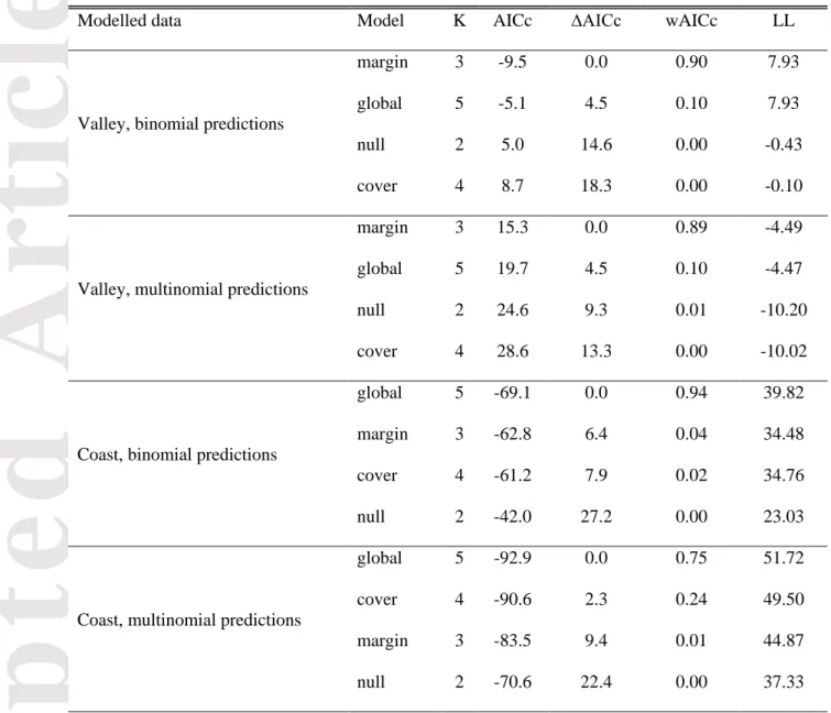
In order to assess how spatially explicit model predictions were supported by field observations, we extracted the predicted probability of transition to shrub dominance (for 2026 in the valley and 2030 on the coast) using the GPS points of the ground-truthing surveys and generated linear models of these probabilities for each of the 4 modelling situations (coast/valley and multinomial/binomial models). We used the shrub cover in the 9 x 9 m quadrat (ordered categorical variable converted to 3 classes, 0-25%, 25-50%, 50-100%) and the presence of an erect shrub stand margin in the 9 x 9 m quadrat (binary variable) as explanatory variables in these linear models. We transformed the shrub cover classes in this way because all cover values above 50% represent shrub dominance and because splitting the values into four even classes would have resulted in only a few values in each of the upper 50-75% and 75-100% classes. Points for which shrubs were already the dominant vegetation type in 2015 or 2016 were not included in the analysis as we were interested in modelling transition probabilities to shrub dominance from other land cover types. A multimodel inference approach was used to identify which of the variables observed in the field (if any) were related to the percent
Accepted
Article
probability of transition to shrub dominance as determined by our land cover modelling exercise. For each of the four transition probability models, we modeled the prediction probabilities using four combinations: cover, margin, cover + margin, and a null model. We ranked these by AICc scores to identify the best model or set of models. Normality and heteroskedasticity assumptions of the global models (i.e. models including all variables) were met in all cases.
GPS points were taken in the field at the central plot locations. However, it sometimes happened that vegetation recorded in the field did not match the 2010 vegetation maps. When this could reasonably be attributed to the precision of the GPS device (between 3 and 5 m), the point was manually moved to a neighboring cell (< 5 m away) so as to be consistent with observations in the field. Comparison of the land cover modelling results to the field observations required that field observations were locally consistent with the variables upon which the model was based for predictions. When such manual edition of GPS point coordinates could not be properly done, the survey point was excluded from the analysis. Overall, data cleaning retained 82 valley survey points and 121 coastal points, of which 14 and 21 points, respectively, had their coordinates manually edited (Appendix S1: Fig. S3).
Satellite-based model corroboration
While field observations enabled validating model predictions at a small scale, we were also interested in testing our predictions against vegetation changes observable at a larger scale. We accessed 30 m-resolution Landsat scenes and assessed how our predictions were consistent with changes in Normalized Difference Vegetation Index (NDVI) over the study area under the assumption that increasing shrub cover is the main driver of NDVI increase. This assumption was based upon patterns observed in other studies (Fraser et al. 2014, McManus et al. 2012) and in this study (see below).
We accessed scenes from WGS frames 19-21 and 20-20 (path-row) using the United States Geological Survey (USGS) GloVis interface. Landsat scenes came from Landsat 5, 7 and 8 and spanned years 1989 to 2016. We chose not to use SLC-off Landsat 7 scenes (scenes collected after
Accepted
Article
May 31, 2003) since they had too much missing data in our study area. Since our study area was relatively small compared to the size of a whole scene, we could filter scenes visually based on whether the study area was covered by clouds or not. We adopted a conservative approach by removing scenes as soon as there were traces of clouds or cloud shadows covering the study area, even when only one of the two zones under study was affected. Scenes that were taken before Julian day 195 or after Julian day 250 (July 14 and September 7 respectively on non-leap years) were
removed from the analysis, as they were likely outside the peak phenology window. Visual analysis of the NDVI data confirmed that there was no relationship between NDVI and the day of the year over the period from Julian day 195 to Julian day 250. Filtering on the basis of cloud cover and day of the year resulted in a set of 27 scenes retained for further analysis (Appendix S1: Table S1).
We converted the red and near-infrared bands to top-of-atmosphere (ToA) reflectance using
coefficients and formulae described in Chander et al. (2009) for TM (Landsat 5) and ETM+ (Landsat 7) data and in the Landsat 8 Data Users Handbook (U.S. Geological Survey 2016) for OLI (Landsat 8) data. NDVI was computed for every 30-m cell according to the standard formula:
NDVI = (NIR - Red) / (NIR + Red)
where NIR stands for the ToA reflectance of the near-infrared band and Red stands for the ToA reflectance of the red band.
To determine whether Landsat data could be used to identify areas where shrubification occurred, we conducted a series of analyses whose aim was to characterize (1) the link between land cover and NDVI as well as (2) the link between land cover transitions and variations in NDVI. We generated mean NDVI rasters for ~1990 by averaging NDVI values of 6 scenes taken in 1989, 1990 and 1992, as well as mean NDVI rasters for ~2010 by averaging NDVI values of 3 scenes taken in 2008, 2010 and 2011. These ~1990 and ~2010 NDVI rasters were used to generate distributions of NDVI values per cover type by superimposing land cover maps from these periods. To avoid land cover
heterogeneity from adding noise to the distribution of NDVI values per land cover type, distributions were generated from sets of relatively homogeneous pixels (30-m Landsat cells comprising at least
Accepted
Article
75% of 5-m pixels of a given land cover type). Since only a few "pure" 30-m water pixels remained, we were not able to generate a distribution of NDVI values for this land cover class.
We also computed NDVI trends by fitting pixel-wise Theil-Sen robust regressions (following Fraser et al. 2014) and considering the regression coefficient for each pixel as a measure of the NDVI trend of that pixel. Theil-Sen regressions for the period 1990-2010 were based on 20 scenes from 13 different years; NDVI values for years for which more than one scene was available were averaged and considered as a single data point. Cells with negative NDVI trends (2.5 % of the 5920 pixels of the valley and 2.3% of the 2180 pixels of the coast) were removed from the dataset as they
corresponded largely to areas where human disturbance (mainly new roads and buildings) was known to have occurred. NDVI trends over the period 2010-2016 were similarly generated using 6 scenes from 5 different years. We first used the NDVI trend data to carry linear regressions modelling the 1990-2010 NDVI trends in a Landsat pixel as a function of the shrub cover increase in that pixel over the same period. For every Landsat pixel, we obtained the percentage of land cover that had
undergone shrubification between 1990/1994 (coast/valley) and 2010. This percentage was obtained by splitting every Landsat pixel into thirty-six (36) 5-m subpixels and determining the proportion of each pixel that had undergone a transition to shrub dominance over the time period considered. We regressed NDVI trend against percentage of shrubification on a regular sample of about 5% of the Landsat pixels (260 pixels in the valley and 103 pixels on the coast). We also assessed where the most substantial increases in NDVI occurred by generating distributions of NDVI trends per initial land cover type (i.e. we generated distributions of 1990-2010 NDVI trends according to the land cover type in 1990/1994 and 2010-2016 NDVI trends according to the land cover type in 2010).
Since the results of the aforementioned analyses (see the Results section) indicated greater NDVI increases in areas undergoing shrubification, we could assess whether our model predictions were consistent with recent NDVI trends by identifying areas that were likely undergoing shrubification according to their 2010-2016 NDVI trends. Generating a dataset to compare these NDVI trends to the spatially explicit model predictions was challenging as both rasters had different projections and
Accepted
Article
extents. To circumvent this, we averaged the 2026/2030 shrubification probability values of the 5 m-resolution raster using a 15 m (3 x 3 pixels) moving window in order to obtain predicted values that were more representative of the general context. We then constructed a dataset associating every 5 m x 5 m pixel to a NDVI trend value by extracting the corresponding value from the 30 m resolution Landsat raster. Cells that were already shrub-dominated in 2010 were excluded from the analysis, as we were interested in transitions to shrub dominance from other land cover types. We fit four different linear models (binomial and multinomial predictions for both the valley and the coast) of NDVI trends as a function of the predicted probabilities of transition to shrub dominance on random samples of about 5% of the number of Landsat cells in the dataset (292 cells in the valley and 104 pixels on the coast). Normality and heteroskedasticity assumptions were met for all linear models involving NDVI data.
Software used
Unless otherwise stated, all analyses and data manipulation were done in R version 3.3.1 (R Core Team 2016). Multinomial logit modelling used the multinom function in package nnet (Venables and Ripley 2002). Binomial modelling used the base glm function with binomial family logit link. Manipulation of spatial data was used packages sp (Pebesma and Bivand 2005), raster (Hijmans 2015) and rgdal (Bivand et al. 2015). Model selection and multi-model averaging used package
AICcmodavg (Mazerolle 2016). Theil-Sen robust regressions were fit using package mblm (Komsta
2013). Computation of the 95% confidence intervals used for the visualization of multinomial model predictions used package effects (Fox 2003, Fox and Hong 2009). AUC values for the binomial models were calculated with package AUC (Ballings and Van den Poel 2013).
Results
Statistical modelling of land cover change
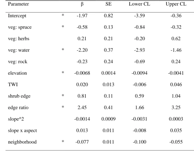
Binomial modelling of land cover change in the valley resulted in two models accounting together for virtually 100% of model weights (Table 3). Confidence intervals (95%) generated using model averaging for parameters included in these two models suggest that vegetation, elevation, shrub edge,
Accepted
Article
edge ratio and neighborhood were important factors associated with shrubification in the valley
(Table 4). Model-averaged values for slope and aspect could not be computed since these were involved in interactions, but confidence intervals computed individually from the best models did not support a role of these variables in shrubification (Appendix S1: Table S2). Transition to shrub dominance was more likely on areas dominated by lichens, herbs and rock outcrops (Table 4). Shrubification probabilities decreased with elevation (Fig. 3a), and increased with increasing edge
ratio (Fig. 3b) and with the presence of a shrub edge (Fig. 3c). Visualization of model predictions did
not support an effect of neighborhood on transition probabilities (Appendix S1: Fig. S4), which is consistent with this variable being found only in the second best model, which was markedly less well supported than the top model.
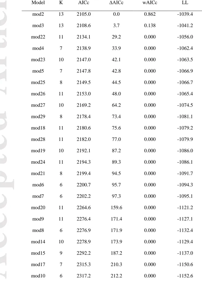
Multinomial modelling of land cover change in the valley identified model 3 as being vastly better supported than any of the 28 alternatives considered (Table 5), so we used it alone for all model inferences and predictions. Interpreting multinomial models is more challenging than binomial models because parameters are estimated for every possible outcome relative to the reference outcome, shrub dominance in this instance. Confidence intervals (95%) generated for the 90 model parameters included in the best multinomial model for the valley suggest an effect of the variables
vegetation, surrounding, elevation, slope, TWI as well as the interaction between slope and aspect on
land cover transitions (Appendix S2: Table S1). As would be expected, the parameters for vegetation indicated that cells tended to remain in their initial land cover class, while the effect of surrounding was to favour transitions to the dominant surrounding cover type. The effect of elevation was consistent with that of the binomial models, with decreasing probabilities of transition to shrub dominance from lichen, spruce and herbaceous cover as elevation increased (Fig. 4a, Appendix S1: Fig. S5. Probabilities of transition to shrub dominance increased on intermediate slopes (10-30°) covered by herbs, whereas steeper slopes were associated to rock outcrops where almost no vegetation can grow (Fig. 4b, Appendix S1: Fig. S6). Transition to shrub dominance was more likely to occur with increasing TWI on lichen-dominated and, to a lower extent, spruce-dominated cover (Fig. 4c, Appendix S1: Fig. S7). The parameter values for the interaction between slope and aspect suggested
Accepted
Article
that transition to shrub dominance on steeper slopes was more likely to occur when these were facing northeast for herb- and rock-dominated areas (Appendix S2: Table S1). The multinomial model also supported evidence for an effect of edge ratio consistent with that observed for the binomial model, specifically that the probability of transition to shrub dominance increased with edge ratio, although it was only significant for lichen and rock patches (Appendix S2: Table S1).
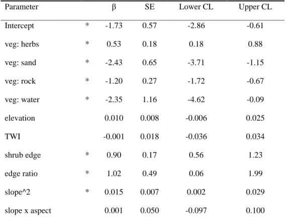
On the coast, binomial modelling of land cover change resulted in a 95% confidence model set comprising four models (Table 6). Confidence intervals (95%) generated using model averaging for parameters included in these models suggest that vegetation, shrub edge, edge ratio and the quadratic term for slope were important parameters in shrubification binomial modelling on the coast (Table 7). As for the valley, model-averaged values for slope and aspect could not be computed since these were involved in interactions, but confidence intervals computed individually from the best models did not exclude 0, so there was no evidence for a role of these parameters (Appendix S1: Table S2).
Transitions to shrub dominance were more likely to occur on herbaceous and lichen cover than on other land cover types (Table 7). The effect of shrub edge was similar on the coast as in the valley, but the effect of edge ratio on predicted probabilities showed only a weak effect of this variable as compared to the valley (data not shown). The effect of the quadratic term for slope was a result of higher probabilities of transition to shrub dominance on slopes steeper than 10° (Fig. 3d), although these represent only 4.8% of the coast area.
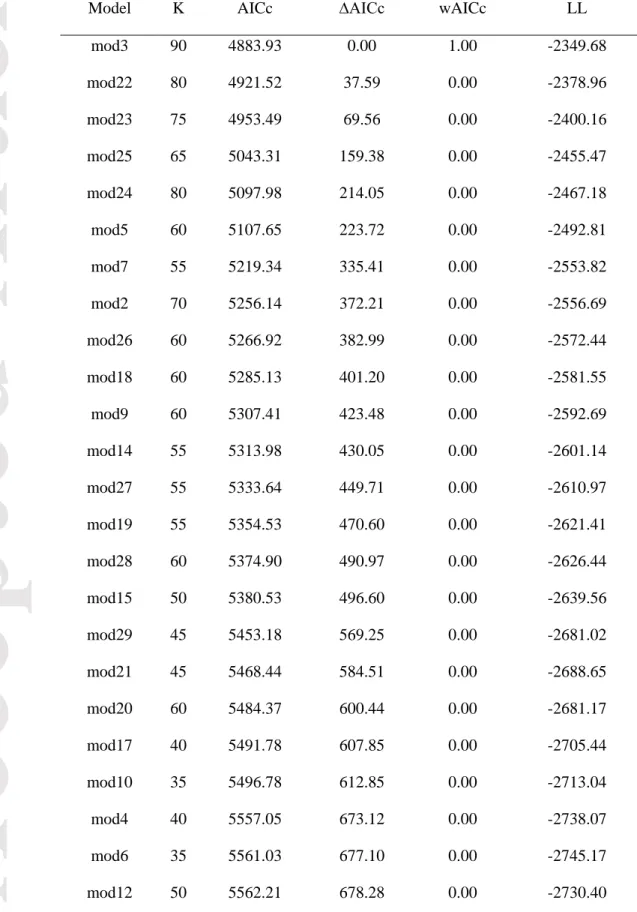
Multinomial modelling of land cover change on the coast also resulted in a single model with virtually 100% of the AICc weight (Table 8), which we used alone for all model inferences and predictions. Confidence intervals (95%) generated for the 80 model parameters included in the best multinomial model for the coast highlight the important effect of vegetation relative to other variables (Appendix S3: Table S1). Compared to the valley, where surrounding was important in modelling transitions to all cover types, the effect on the coast was only significant for rock and herbaceous cover (Appendix S3: Table S1). Apart from a higher probability of transition from herbaceous and sand cover to shrub dominance with increasing elevation (Fig. 4d, Appendix S1: Fig. S8) and a higher probability of
Accepted
Article
transition to shrub dominance for lichen-dominated patches facing northeast (Appendix S3: Table S1), there was no conspicuous effect of topographic variables on multinomial transition probabilities on the coast.
Spatially explicit modelling of land cover change
Spatially explicit shrubification probabilities for 1990/1994 - 2010 were estimated from binomial and multinomial models for both the valley and the coast (Fig. 5) and were used to generate spatially explicit predictions. AUC values for the binomial models of the valley and the coast were 0.77 and 0.74, respectively, which indicates a fair predictive capability for these models (Swets 1988). The overall accuracies of our spatially explicit predictions (corresponding to 1 minus the total
disagreement presented in Fig. 6) ranged from 58.7% to 76.9%. Quantity and allocation disagreement values for all eight types of spatially explicit predictions indicate that most of the inaccuracy of our predictions stems from allocating pixels to the wrong class rather than allocating the wrong number of pixels in each class (Fig. 6). Spatially explicit maps generated from deterministic realizations of the statistical model predictions were consistently better (in terms of total disagreement) than those generated from stochastic realizations, although stochastic realizations tended to perform better than their deterministic counterparts in terms of quantity disagreement (Fig. 6). Interestingly, multinomial stochastic models resulted in almost perfect quantity agreement while resulting in the worst allocation disagreement (Fig. 6). Moreover, stochastic realizations resulted in highly pixelized maps that we deemed rather unrealistic representations of the vegetation change processes underway in the region (results not shown). Deterministic multinomial models generated slightly better spatially explicit predictions than binomial models (Fig. 6), but given the much higher number of parameters that have to be estimated, the significance of the minor improvements is questionable. Predictions were
consistently more accurate for the valley than for the coast according to total disagreement, but these differences were less pronounced when looking at kappa coefficients (Fig. 6). This is likely a
consequence of the higher proportion of shrub dominance in the valley, which makes it more likely to accurately predict a cell as being shrub-dominated.
Accepted
Article
Based on the preceding results, long-term predictions of the proportion of land dominated by different cover classes over time were generated from the deterministic models. Predictions for both the valley (Fig. 7a) and the coast (Fig. 7b) were marked by an increase of shrub cover, mainly at the expense of lichen and herb cover. Predictions generated from binomial and multinomial models were roughly similar, except for the proportions of rock and herbaceous cover on the coast, which differed markedly between the two models (Fig. 7b). The models tended towards equilibrium of the proportions of land in different land cover classes, presumably as the most probable vegetation conversions had all occurred by the end of the simulation period.
Field-based model corroboration
Comparison of the model predictions for 2026 in the valley with the data collected in the field ranked the model with only margin as the best model both for the binomial and multinomial predictions (Table 9). Based on AICc weights, there was no support for an association between shrub cover and model predictions. Quadrats on the margin of a shrub patch in the field had higher predicted
probabilities of shrubification than others, even though there was considerable overlap between the probability values (Fig. 8a). On the coast, binomial model predictions were best modelled by the global model which included both margin and shrub cover, as evidenced by the ranking of the global model as the best model (Table 9). Multinomial model predictions for the coast were best modelled by the global model as well. Among the univariate models, there was better support for an effect of shrub cover in the field than for margin (Table 9). Predicted shrubification probabilities, both from binomial and multinomial models, were higher on the coast when shrub cover was also higher in the field (Fig. 8b).
Satellite-based model corroboration
Different land cover types clearly differed in the distribution of their NDVI values, with NDVI values decreasing roughly as expected in the following order: shrubs > spruce > herbs > lichen > rock > sand (Appendix S1: Fig. S9). Although increasing trends were observed for all land cover types, higher NDVI increases over the period 1990-2010 were observed in areas where the vegetation was initially
Accepted
Article
herb- or lichen-dominated, both in the valley and on the coast (Appendix S1: Fig. S10); these cover types also correspond to the ones that underwent the most important transition to shrub dominance over the same period. Similar tendencies were not observed for the 2010-2016 NDVI trends (Appendix S1: Fig. S10), which proved to be markedly higher than 1990-2010 trends (see also the maps of Appendix S1: Fig. S11). We found significant positive linear relationships between NDVI trends and percentage shrubification for both the valley (β = 0.004, P < 0.001; Appendix S1: Fig. S12) and the coast (β = 0.005, P < 0.001; Appendix S1: Fig. S12), although the proportional explained variance was low (R2 of 0.11 and 0.20, respectively). Among the four linear models constructed in order to assess the link between model-predicted probabilities and 2010-2016 NDVI trends, only the models of the coast showed a significant relationship between NDVI trends and predictions (Binomial predictions: β = 0.01, P < 0.01, R2 = 0.07; Multinomial predictions: β = 0.01,
P < 0.01, R2 = 0.06; Fig. 9), although the explained variance was very low. The two models of the valley did not yield evidence for a relationship between binomial nor multinomial predicted values and 2010-2016 NDVI trends.
Discussion
Topographic drivers of shrubification
Recent research on the spatial patterns of shrubification underlines the importance of topography, hydrology and disturbance as drivers of this phenomenon at the landscape scale. A unifying paradigm from much of this research is that shrub growth and recruitment are enhanced where both nutrients and water are not limiting (Tape et al. 2012) and where climate conditions are milder (Swanson 2015). Shrub stands usually grow higher and expand more rapidly along drainage features (Naito and Cairns 2011, Tape et al. 2012, Curasi et al. 2016) and dendrochronological data (Myers-Smith et al. 2015) show that the climate sensitivity of shrub growth is higher in wetter areas. Tape et al. (2006) observed that the rate of shrub cover increase differed from one valley system to another and among different topographical units, hill slopes and valley bottoms being more liable to shrubification than interfluves. Ropars and Boudreau (2012) similarly found that shrub cover increased more rapidly on
Accepted
Article
river terraces than on hilltops. Aerial photography analyses by Tremblay et al. (2012) and Cameron and Lantz (2016) also yield evidence for a higher shrubification rate at lower elevation sites, although increases in shrub cover tend to also occur at higher elevations. Increasing disturbance from human activity (Fraser et al. 2014, Cameron and Lantz 2016), fire (Lantz et al. 2013), or geomorphological processes (Lantz and Kokelj 2008, Lantz et al. 2009) also enhance shrub growth and recruitment by increasing nutrient availability and exposing favourable seedbeds.
Our results are in accordance with previous research in emphasising the importance of topographical variables in the control of shrub expansion in subarctic ecosystems. In the valley, we found that shrub cover is more likely to increase at lower altitudes, as was observed in previous studies (Tremblay et al. 2012, Cameron and Lantz 2016). Lower elevation sites in the valley are largely sheltered from the wind and are characterized by numerous drainage features and wetter areas where shrubs can thrive. On the contrary, the lichen-dominated plateau overlooking the valley is characterized by shallow soils and high wind exposure unfavourable to the development of erect shrub stands. Field observations of our research group on this plateau suggest, however, that shrub cover and size have increased recently and that B. glandulosa is ubiquitous even though aerial photography has not detected a switch to shrub dominance in this area between 1994 and 2010. These observations in the field are supported by our analysis of 2010-2016 NDVI trends, which show that large increases in NDVI have occurred on the plateau over this period (Appendix S1: Fig. S11). It is likely that shrub dominance will also increase on the plateau, although the timespan of our study did not allow our modelling exercise to detect significant changes in this area. Whether shrubs will remain low or will develop into high shrub stands in this area is of interest, since the ecological impacts of shrubification occur mainly in high shrub stands (Myers-Smith and Hik 2013, Paradis et al. 2016).
The influence of elevation on land cover changes was not as obvious on the coast as in the valley. This was expected, as the elevation range on the coast 45 m a.s.l.) is narrower than in the valley (0-180 m a.s.l.). Multinomial modelling of land cover change for the coast found an effect opposite to the one observed in the valley, with increasing probability of transition to shrub dominance with elevation
Accepted
Article
on herbaceous and sand cover. This effect is likely due to increasing distance from the sea with increasing elevation on the coast; areas farther from the coast are more sheltered from the wind and therefore more likely to favour shrub recruitment and growth. The higher probability of shrub colonization on northeast-facing lichen patches also supports the interpretation that the influence of the sea plays an important role in land cover transitions on the coast, since patches facing northeast are sheltered from the wind coming from the sea. Erosion by ice and water also prevent shrub colonization of the sandy beach running along the coast, which explains this effect of elevation on transition to shrub dominance on sand cover.
We expected to find a conspicuous positive effect of topographic wetness index (TWI) on
probabilities of transition to shrub dominance for both study areas, since this variable has been linked to shrubification in a previous study (Naito and Cairns 2011) and shrub performance is related to water availability (Tape et al. 2012, Cameron and Lantz 2016, Curasi et al. 2016), but a significant effect of TWI was only observed on lichen and spruce cover in the valley. However, a weak effect of TWI does not mean that shrub growth and recruitment does not depend on moisture conditions in our study system. TWI is a measure of soil moisture potential based entirely on topography, but soil moisture content depends on other factors such as soil physicochemical conditions and vegetation structure and community (Ben Wu and Archer 2005). The effects of slope and aspect found by our models, on the other hand, do support a role of water availability in shrub cover increase. An interesting pattern revealed by the valley multinomial model was an increase in the probability of transition to shrub dominance on moderate slopes (10-30°) dominated by herbs. Binomial models for the coast also found a higher probability of shrub dominance on slopes steeper than 10°. Both in the valley and on the coast, such conditions are mostly found in the vicinity of drainage features characterized by high water and nutrient availability while being well drained. Moreover, these depressions probably accumulate more snow in the winter, enabling deeper permafrost thaw and moisture availability from snowmelt in the spring and summer while also protecting shrubs from winter frost damage (Ropars et al. 2015a). In the valley, the higher probability of shrub dominance on
Accepted
Article
herbaceous and rock slopes exposed to the northeast is also likely due to higher moisture and snow accumulation on these slopes because of lower exposure to sunlight.
Spatial arrangement of land cover as a driver of shrubification
Previous research has documented that the rates of shrub cover and growth increase depended on the type of environment or vegetation in which they grow. Patterns emerging from aerial photography analysis commonly show an increase in shrub cover at the expense of lichen-dominated areas (Ropars and Boudreau 2012, Fraser et al. 2014), an observation consistent with the decreases in lichen cover expected with climate change (Cornelissen et al. 2001, Elmendorf et al. 2012a). On the other hand, shrubs usually perform poorly in tussock tundra, where inadequate drainage, acidity and a shallow active layer inhibit the development of a vertical structure (Tape et al. 2012, Swanson 2015).
We found strong support for effects related to land cover type and the spatial arrangement of
vegetation. Land cover type at a given time was an important predictor of the land cover type at a later time in both study areas. Land cover type identifies which state a given cell is most likely to remain in as well as how likely different transitions are. In the valley, most of the low-elevation (as opposed to those found on the plateau) lichen expanses occur on permafrost mounds that, upon thawing, create moisture and microtopographic conditions favourable to shrub growth (Schuur et al. 2007,
Provencher-Nolet et al. 2014) whereas on the coast, shrub encroachment on lichen-dominated areas appeared to result mainly from clonal propagation of shrubs on well-drained sites. Model results also supported some degree of shrub encroachment on herbaceous vegetation, although identifying the reasons for these shifts is more complex as there is considerable heterogeneity in this land cover class. It seems likely that herbs in well-drained sites will progressively yield to shrub dominance, but the fate of poorly drained areas is less clear. Observations of large numbers of shrub seedlings in the field indicate high recruitment in moist areas dominated by grasses and sedges (pers. obs.), although their low height raises questions as to whether shrubs will reach dominance in these sites.
Accepted
Article
The proximity of shrub-dominated cells was closely associated with transition to shrub dominance in binomial models, while the major surrounding land cover type was a relatively important predictor of land cover transitions in the multinomial model of the valley. The link between these variables and transition probabilities underline the importance of neighborhood effects in the prediction of
vegetation change. Repeat photography studies consistently show shrub cover increases in the vicinity of existing patches (Sturm et al. 2001, Myers-Smith et al. 2011b, Lantz et al. 2013) and Tape et al. (2012) observed that expanding shrub patches tend to adopt a clumped configuration. These neighborhood effects could result from the clonal propagation of shrub patches or preferential recruitment near mature patches, such that sites are more easily colonized by shrubs when expanding patches are found in their surroundings. Another explanation (which does not exclude the former) is that environmental conditions (soil properties, wind exposure, exposure to sunlight, topography, etc.) are more likely to be similar in neighboring cells, so that areas adjacent to shrub patches may be more suitable for shrub growth than would be randomly picked sites elsewhere in the landscape. The effect of edge ratio, which was an important predictor of binomial models of the valley, is similarly related to land cover change, as it is a measure of the exposure of a vegetation patch to other land cover types. Smaller and more irregularly shaped patches (i.e. patches with a higher edge ratio) will likely be more liable to colonization by shrubs since they are more exposed to shrub edges, although it might also be that they were irregular because they were more liable to shrubification in the first place.
Overall performance of the models
The models generated in our study were satisfactory in their explanatory power. AUC values over 0.7, such as those computed for our binomial deterministic models, indicate that models can prove useful for “some purposes” (Swets 1988; we can take this to include highly complex ecological systems) and although such values could not be computed for multinomial models, these showed similar
performance to binomial models based on kappa coefficients and disagreement values. Predicted binomial and multinomial probabilities also showed good visual agreement with their respective shrubification maps over the same time periods (Fig. 5). Our results indicate that our models
Accepted
Article
performed much better at predicting the fraction of land cover dominated by different classes than at predicting the class that will dominate a given pixel later in time. This is likely to be the case for models like ours since allocation disagreement can result both from predicting change in pixels that did not change between 1990/1994 and 2010, and from predicting stability for pixels that did change. These results suggest that our deterministic models are likely to be an accurate representation of changes that are likely to happen in the future, although they are limited in their fine-scale predictive capacity.
Comparing results of predictions among studies is difficult because they are interested in different phenomena, spatial scales, time intervals, and change rates. Moreover, models used in land cover change prediction vary largely from one study to another, and different authors usually report different statistics to assess the performance of their models. Nonetheless, the performance of our models can be considered in the range of that obtained in other studies interested in similar processes. Pueyo and Bueguería (2007), in a study modelling secondary succession following farm abandonment in Spain, generated binomial models with AUC values ranging from 0.76 to 0.83 and an overall prediction accuracy of 67.8%. Rutherford et al. (2007), in a study modelling similar transitions in Switzerland, obtained AUC values ranging from 0.5 to 0.78. Upshall (2011), who reported results from a Markov-cellular automaton model also interested in shrubification, reported an overall prediction accuracy of 70.8% and a kappa coefficient of 0.66. We suggest that future studies of land cover change modelling should report at least AUC values since these are independent of outcome frequencies (Swets 1988) and are thus more easily compared among studies. As discussed in Rutherford et al. (2007), prediction accuracies and kappa coefficients remain useful for model performance interpretation, and we suggest authors to also report these statistics along with quantity and allocation disagreement when describing the results of land cover change models.
Stochastic versus deterministic modelling
Deterministic models performed better than stochastic models when translating statistical model predictions into actual predictive maps, based on both overall accuracy values and kappa coefficients. Stochastic predictions also resulted in unrealistically pixelized maps, a well-known problem in spatial
Accepted
Article
modelling (Weaver and Perera 2004) that could not be corrected in our modelling exercise by variables taking the spatial context into account (e.g. shrub edge and surrounding). Deterministic model realizations were similarly found by Carmel et al. (2001) to generate predictive maps that match observed maps better, although stochastic realizations might outperform deterministic ones when predicting proportions of different cover classes, as was the case here for maps arising from stochastic multinomial models.
Binomial versus multinomial modelling
We tested both binomial and multinomial models of vegetation change in the Umiujaq region in order to assess whether land cover transitions could be represented merely as a shrubification process (conceptualized as a binomial model) rather than the whole spectrum of land cover transitions (conceptualized as a multinomial model). It appears from our results that the small increase in performance obtained from modelling a multinomial process instead of a binomial one does not justify the ~ 5-fold higher number of parameters used in multinomial models. Moreover, long-term predictions generated from binomial and multinomial models were largely similar to one another. Our results thus indicate that neglecting changes other than transition to shrub dominance does not result in a reduction of prediction accuracy, which lends strong support for the significance of the
shrubification process currently observed at the circumpolar scale. This reaffirms shrubification as the major component of land cover change in subarctic regions and reinforces the importance of
understanding the impacts of this phenomenon on feedbacks to climate due to changes in energy fluxes between the ground and atmosphere, permafrost degradation and reduction of lichen and moss cover, among others. Multinomial models generated in our study still enabled us to reveal
ecologically meaningful patterns related to the effects of slope and aspect in the valley and elevation on the coast that would have remained concealed had we only generated binomial models. Thus, although multinomial models were not essential to generating accurate predictions of land cover changes, they were still useful in order to gain understanding about the shrubification process.