Worldwide wavelet analysis of geomagnetic jerks

HAL Id: hal-01914561

https://hal.archives-ouvertes.fr/hal-01914561

Submitted on 20 Sep 2019

HAL is a multi-disciplinary open access

archive for the deposit and dissemination of

sci-entific research documents, whether they are

pub-lished or not. The documents may come from

teaching and research institutions in France or

abroad, or from public or private research centers.

L’archive ouverte pluridisciplinaire HAL, est

destinée au dépôt et à la diffusion de documents

scientifiques de niveau recherche, publiés ou non,

émanant des établissements d’enseignement et de

recherche français ou étrangers, des laboratoires

publics ou privés.

Worldwide wavelet analysis of geomagnetic jerks

Mioara Alexandrescu, Dominique Gibert, Gauthier Hulot, Jean-Louis Le

Mouël, Ginette Saracco

To cite this version:

Mioara Alexandrescu, Dominique Gibert, Gauthier Hulot, Jean-Louis Le Mouël, Ginette Saracco.

Worldwide wavelet analysis of geomagnetic jerks. Journal of Geophysical Research, American

Geo-physical Union, 1996, 101 (B10), pp.21975 - 21994. �10.1029/96JB01648�. �hal-01914561�

JOURNAL OF GEOPHYSICAL RESEARCH, VOL. 101, NO. B10, PAGES 21,975-21,994, OCTOBER 10, 1996

Worldwide wavelet analysis of geomagnetic jerks

Mioara

Alexandrescu,

1 Dominique

Gibert

2 Gauthier

Hulot

1

Jean-Louis

Le Mou;S1,1

and Ginette

Satacco:

Abstract. Following

an earlier

study

which

gives

the principles

of the method

and an example

of application

to the eastern

component

of the magnetic

field

in

the European

region

[Alexandrescu

et al., 1995],

detection

and

characterization

of

geomagnetic

jerks

using

wavelet

analysis

is generalized

to any

horizontal

component

of the field and to a worldwide

distribution

(involving

97 locations)

of observations.

This allows

for a systematic

and global

search

for such

events

within

the twentieth

century

and

makes

it possible

to unravel

a number

of intriguing

properties

associated

with them. Whereas

our first study only reveals

five such

events

in Europe, we can

now state that seven

and only seven

events

have apparently

occurred

throughout

the world

during

the present

century.

Two (1969

and 1978)

are unquestionably

of

global

extent,

three

(1901,

1913,

and

1925)

being

possibly

of similar

extent,

while

the remaining

two (1932

and

1949)

are not seen

everywhere

at the Earth's

surface.

We confirm

our early result

that the events

are more

singular

than previously

thought,

with a "regularity"

systematically

closer

to 1.5 than

to 2, and

a common

mean value of about 1.6. Furthermore,

the 1969 and 1978 events

display a two-step

spatio-temporal

behavior

consisting

of an "early

arrival"

in the

northern

hemisphere,

a "late arrival" in the southern

hemisphere,

and a time lag between

the two arrivals

of the order

of a couple

of years.

We were

also

able

to show

that the 1969

and 1978

events

tend to at least

partially

balance

each

other. The extent

to which

this is true

remains

to be assessed,

mainly

because

our method,

although

already

providing

some

information

about

the geometry

of the events,

does

not yet allow

the proper

recovery

of their intensities.

Introduction

Assessing

the exact

nature

of the time changes

of the

magnetic

field of internal

origin

at the surface

of the

Earth and at the core-mantle boundary is important,

not only for its own sake but also for the information

it can give

about

the deep

Earth, such

as the electrical

conductivity

of the lower mantle, the motions

at the

core and the mantle.

The identification of an abrupt change in the trend

of the geomagnetic

secular

variation,

referred

to as a

"jerk"

[Courtillot

et al., 1978;

Malin et al., 1983],

and

the demonstration that it really is of internal origin, re-

quired

quite

some

efforts

in the past

years.

This inter-

nal origin

now

seems

to be well

established.

Malin and

Hodder

[1982]

devised

a filter

to measure

the magnitude

of the 1970 discontinuity

in the second

time derivative

•Institut de Physique du Globe de Paris, Paris, France.

2G6osciences Rennes -- Centre National de ia Recherche

Scientifique/Institut National des Sciences de l'Univers, Rennes.

France.

Copyright 1996 by the American Geophysical Union.

Paper number 96JB01648.

0148-0227/96/96JB-01648509.00

of the field components at 83 observatories; performing a spherical harmonic analysis of these magnitudes led them to conclude that most of the sudden change is in-

deed of internal origin. Gubbins and Tomlinson [1986]

removed the external field effects from the data and at-

tributed the discontinuity in the time derivatives of the

resulting time series to an internal origin. Gavoret et al.

[1986] analyzed monthly mean values and also stressed the internal nature of the phenomenon.

However, the definition and characteristics of the ge- omagnetic jerks are still a matter of debate in the ge- omagnetic community. Even the fundamental parame- ters of a jerk, such as the date at which it occurs, the time duration of the impulse, or the worldwide char- acter of the event are not agreed upon by all the re-

searchers.

The late 1960s event has for instance been reported as

occurring in 1969 [Courtillot et al., 1978; Courtillot and Le Mou•'l, 1984; McLeod, 1985, 1989; Golovkov et al., 1989], 1970 [Stewart and Whaler, 1995], or 1971/1972 in the Australian region [Gubbins and Tomlinson, 1986; Whaler, 1987]. Another sudden change in the secular

acceleration of the geomagnetic field has been reported

around 1978 [Gavoret et al., 1986; Gubbins and Tom-

linson, 1986; Langel ½t al., 1986; McLeod, 1989; Stewart and Whaler, 1995]. Stewart [1991] indicated the exis-

tence of another jerk in 1983, also detected in South

21,976 ALEXANDRESCU ET AL.' WAVELET ANALYSIS OF GEOMAGNETIC JERKS

Africa by Kotzd et al. [1991] and on South Georgia island by Dowson et al. [1988]. Other jerks have also been detected earlier in this century: in 1913 [Courtillot

and Le Mou•'l, 1984; Ducruix and Le Mou•'l, 1983; Give

et al., 1984]

and in 1925 [McLeod,

1989],

and a number

[McL½od,

1989], 1937, 1947, and 1958 [Golovkov

½t al.,

ropean area and using the wavelet analysis of monthly mean values, five and only five events have been de- tected since the beginning of this century: around 1902,

1913, 1925, 1969, and 1978 [Alcxandrescu et al., 1995].

As this method has been proved to be objective and efficient, we now present a systematic and worldwide analysis in order to exactly assess the existence, timing

(and possible

regional

delays),

and general

characteris-

tics of such events.

A good determination of the duration (which can be

defined as the time needed for the change of slope in the

time series of the secular variation to be completed), and time of occurrence of these events is very much re-

quired. A change of the core field in a time span of about a year or less would, for instance, shorten the period of variations of internal origin as given by early

estimates [Curvie, 1967, 1968; Alldredge, 1984]. Also,

the effect of the conducting mantle could be addressed

with better data. Backus [1983], who discussed the fil-

tering effect of the mantle and suggested that it behaves

as a causal time-invariant real linear filter, noted that the centroid date (emergence time) and smoothing time

of the jerk could be different at different locations at the

Earth surface, even in the case of an ideal jerk occur-

ring at the core-mantle boundary. A study of the jerks using a time sampling which could resolve these differ-

ences would therefore prove very valuable.

Up to now most studies focused on the European re- gion [Ducruix et al., 1980; Achache ½t al., 1980; Gayover ½t al., 1986] which has by far the best coverage of ob-

servatories and for which the impulse field usually has

a strong Y (east) component. But impulses are also known to be found in other components and elsewhere [see Courtillot and Le Mou•'l, 1988]. Analyzing only

the usual orthogonal components of the geomagnetic

field (X, Y, Z) may mean that impulses might have been masked at some places due to this choice of axes. In the present study we will therefore extend our previous analysis [Alcxandrescu et al., 1995] (hereinafter referred

to as paper 1) to worldwide data and apply the wavelet

analysis to linear combinations of the horizontal com- ponents (X and Y), in order to better estimate the characteristics of the jerks.

brief description of the main aspects of the method is

given in the appendix. A significant difference with our previous study is that the present analysis is no longer restricted to the Y component. It is generalizer' and aims at recovering the direction and sense of the hori-

zontal component of the jerk.

Now, as in paper 1, we will assume that the signal

recorded in the observatories is the sum of a main-field

signal containing singularities, that is, jerks, an exter- nal long-period signal, and noise. In paper 1 we de- composed the analyzed Y component in the following

canonical form:

v (t) =

(t)+

(t)+

(t),

where /•j• is the jerk signal (it represents an abrupt

change with a regularity c• and intensity • localized at

the time to):

j•(t)-

{ 0

(t-to) •

t_<to (2)

t>to

'

h¾ is the Y component of the "periodic" external signal and n¾ the noise on the Y component. Let us now gen- eralize this decomposition to the horizontal component

•(t) of the

field.

The

external

signal

-• can

reason-

its characteristics along this particular direction.

We will therefore assume that

x(t) ¾(t)

- /• cos(0)j• (t) + cos(g)h (t) + nx (t), (3)

-

/• sin(0)j• (t) + sin(g)h (t) + n¾ (t). (4)

The noise will be considered as being isotropic. The

angle 0 (counted eastward from the geographical north direction) will be called the direction angle of the jerk;

• the direction angle of the external signal.

The first step of the analysis consists in computing a set of linear combinations of the original components:

fa, (t) - cos(e')X (t) -3-

sin(e')Y (t),

(5)

step consists of taking the wavelet transform of the sig-

nal (see the appendix). The linearity of the wavelet transform implies that

Method of Analysis

Detection of Singularities With Wavelets

The theoretical background is identical to the one described in paper 1, except for a few details, and the reader is referred to this paper for a full description of wavelet analysis applied to singularity detection. A

For a rotation angle 0' - 0e - 0 + zr/2, the jerk is re-

ALEXANDRESCU ET AL.' WAVELET ANALYSIS OF GEOMAGNETIC JERKS 21,977

form of the rotated signal

fo• (t) is limited to the one of

Wfo,(t,a) -- cos(- O,)Wh(t,a)

+W [nx sin(0,) + r/y COS(0e)]

(t, a).

In this case,

and in view of the results

obtained

in paper

1, all ridge functions

extracted

from the wavelet

trans-

form Wfo, (t, a) should

be either

of type 2 (i.e., typical

of the harmonic

signals)

or of type 3 (i.e., strongly

al-

tered

by the random

noise);

see

the appendix.

If the rotation

angle

is now O' = Ob

= • + •r/2,

..6 6 6 o rot=180 2 4 6 2 4 6 2 4 •. ,,•.6 6 6 0 2 4 6 2 4 6 2 4 •'6 6

o,

o

1

•

rot=50

=

Log2(dilation) Log2(dilation) Log•(dilation)

Figure 1. Ridge functions for the 1947 artificial jerk injected in the CLF series and computed for 0' spanning [0 ø, 180 ø] in steps of 10 ø. The ridge functions of type

2 observed for 0' - 130 ø and 140 ø correspond to the

extinction of the jerk (as detected in Plate 1). Good

quality ridge functions of type i are observed for 40 ø _<

0' < 90 ø.

Wfs•(t,a) -- /•cos(0-0b) Wja(t,a)

-}-W [r/X COS(0b) -}- r/y sin(0o)] (t, a), (8)

the contribution of the wavelet transform of the har-

monic signal disappears and the ridge functions of type 1 associated with the jerk should be better detected in

the wavelet transform W fob (t, a).

Assessment of the Method

We now give several synthetic examples to illustrate the theoretical considerations developed in the preced- ing section. As already mentioned, the results presented in this study have been obtained with the same analyz- ing wavelet as in paper 1. However, in order to obtain the most reliable assessment of the method, we did not use the harmonic signal and synthetic noise described

in this previous paper. Instead we used data extracted directly from six European observatories (BFE, CLF, ESK, HAD, LER, NGK) and covering the 1925-1970 period displaying no jerk (in Europe). To these time

series, considered to be typical real signals free of any jerks, was superimposed a synthetic jerk with a regu- larity c• - 1.65 and a strength /• - 0.17 nTxmonth -• estimated from the 1969 jerk detected in the Chambon-

la-For•t

Y series

(see

equation

(12) of paper

1).

We set 0 - rr/4, and the synthetic jerk was succes-

sively injected at 1943, 1945, 1947, 1949, and 1951 in order to look for some possible influence of the relative phasing of the external signal with respect to the jerk. From the previous section we can expect that both the date and the regularity of the jerk should be best es-

timated for 0 • - 0• - • + rr/2, and the jerk removed for 0" - 0e - 0 + 7r/2. This was checked very efficiently

using the movie procedure included L• the seismic pro- cessing package distributed by the Center for Wave Phe-

nomena at the Colorado School of Mines [Scales, 1995]. This is the way we determine the direction 0 of the

jerk. The sign of the jerk along this direction can then be recovered by inspection of the sign of the wavelet

transform (see the appendix). In this way we finally

get local characteristic directions for the jerk.

An example of a movie sequence represented at 10 ø intervals for the CLF series and the 1947 synthetic jerk is shown on Plate 1. Such sequences have actually been

computed for 5 ø increments (not shown on Plate I for reasons of space) in order to accurately detect the ex-

tinction of the jerk which is clearly achieved within a

limited range (10 ø) of angles 0 • around 0 q- rr/2. The

signature of the jerk is visible for a wide range of an- gles 0 • centered on 0• in the form of a conelike patch of large amplitude. A precise determination of both the date and the regularity c• of the event can be obtained from the ridge functions displaying the best type 1 be-

havior (Figure 1, which displays the 18 ridge functions corresponding to the sequence shown in Plate 1).

Since the appearance of the jerk is not as sudden as its extinction, type 1 ridge functions can be observed

within an interval of 0 • of some tens of degrees. The center of this interval depends on both 0 and •, and

21,978 ALEXANDRESCU ET AL.: WAVELET ANALYSIS OF GEOMAGNETIC JERKS 1030 1940 1950 1960 1970

Time (years)

Time (years)

,,..,,8•

100

Time (years)

Time (years)

Time (years)

Time (years)

,11

170

':,

:,..

...

?I .

Time (years)

Time (years)

.{{? .•

ß

Time (years)

150

,..,•] •o

.

Time (years)

Time (years)

Time (years)

Time (years)

Time (years)

Time (years)

Time (years)

193o 194o 195o 196o

Time (years)

30

1980 1940 1950 1960

ALEXANDRESCU ET AL.' WAVELET ANALYSIS OF GEOMAGNETIC JERKS 21,979

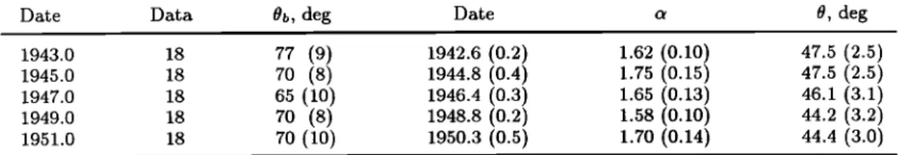
Table 1. Results of the Synthetic Tests

Date Data 0b, deg Date O, deg

1943.0 18 77 (9) 1942.6 (0.2) 1.62 (0.10) 1945.0 18 70 (8) 1944.8 (0.4) 1.75 (0.15) 1947.0 18 65 (10) 1946.4 (0.3) 1.65 (0.13) 1949.0 18 70 (8) 1948.8 (0.2) 1.58 (0.10) 1951.0 18 70 (10) 1950.3 (0.5) 1.70 (0.14) 47.5 (2.5) 47.5 (2.5) 46.1 (3.1) 44.2 (3.2) 44.4 (3.0)

Numbers in parentheses are standard deviations.

gives a poor estimate of 0b (to determine 0b more ac-

curately, we would symmetrically look for the direction

• + •r/2 which extinguishes the harmonic type ridge function).

Now, for the six previously mentioned synthetic se- ries, we retrieved the extinction angle 0e and examined the best type 1 ridge functions. The statistics of the results for the five injection dates are summarized in Table 1. These statistics include the three best type 1 ridge functions for each observatory. It appears that the method allows the recovery of the regularity a with a relative uncertainty of about 10% and the extinction angle 0e within an error of the order of 5 ø. The dat- ing of the jerks should ideally be done using the lines of extrema for very small dilations where the time localiza-

tion of the wavelets is more precise (see the appendix).

In practice, we use the smallest dilations unaffected by the noise and corresponding to the small-dilation end

of the linear

part of the ridge

functions

(i.e., a •_ 23'5

as

trema corresponding to the analyzed ridge functions of

type i (Table 1) is shown on Figure 2. At small dilations

(a g 23'5),

the lines

are controlled

by the noise

and are

scattered. For the dilation range corresponding to the

linear part of the ridge functions

(a • 23'•), the lines

characterizing each date of artificial jerk are well local-

ized within a time interval smaller than 1 year. How-

ever, this part of the lines of extrema form curved arches with their large-dilation end located at dates about 2 years before the theoretical dates. The statistics show

that the dates obtained for the smallest dilation avail-

able (i.e., a •_ 23'•) fall within an interval

of about 6

months and that, due to the curvature of the lines of extrema, the average dates obtained are slightly biased

(less

than 6 months) toward the inferior dates (Table

1). Therefore

in what follows,

dilations

a •_ 23'• will be

used for dating the real jerks.

Data Selection

The present study has been performed on observa- tory monthly means (defined as being the average over

all days

of the month and all times of the day) obtained

from the National Geophysical

Data Center (NGDC,

In the latter case the data were either obtained in digi- tal form or digitized from year books. For the purposes of the present study the first criterion in data selection was the length and continuity of the time series of the

northward (X) and eastward (Y ) components (available or computable from declination (D) and horizontal in- tensity (H)). Only observatories for which time series

were available over a continuous time interval longer than 12 years have been selected. We had to accept some gaps in some of the series and, in these cases, a linear interpolation was used to reconstruct the missing values; the largest gaps we corrected for were 6 months long. In the case of a longer gap the time series was

split into two.

Following this initial selection, all time series were subjected to a careful validation procedure using the

wavelet transform as in paper 1. When anomalies were

)42 1944 1946 1948 1950 19'52

Time (years)

Figure 2. Lines of extrema extracted from the wavelet transforms computed from the five artificial jerks in- jected at 1943, 1945, 1947, 1949, and 1951 into the BFE,

CLF, ESK, HAD, LER, and NGK data series. Only the best three lines are drawn (see text for details). For each artificial jerk the average of the lines of extrema (solid lines) indicates the time of occurrence (see also Table 1). Also shown are the standard deviations of the lines of extrema (dashed curves).

Plate 1. Wavelet transforms of the 1947 artificial jerk injected in the CLF series and computed for 0 • spanning [0 ø, 180 ø] in steps of 10 ø. The extinction of the jerk begins for 0• = 100 ø and

it is complete for • = 130 ø The color scale represents the sign of the wavelet transform: red indicates positive, blue indicates negative.

21,980 ALEXANDRESCU ET AL.' WAVELET ANALYSIS OF GEOMAGNETIC JERKS

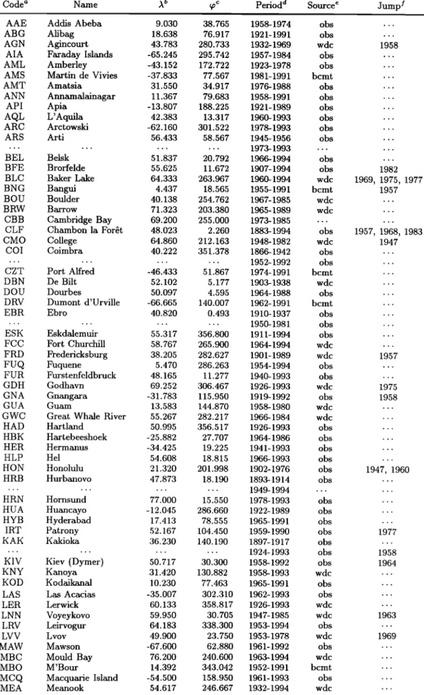
Table 2a. Observatories Considered in the Present Study

Code" Name • b ½ c Period a Source Jump !

AAE Addis Abeba 9.030 38.765 1958-1974 obs

ABG Alibag 18.638 76.917 1921-1991 obs AGN Agincourt 43.783 280.733 1932-1969 wdc

AIA Faraday Islands -65.245 295.742 1957-1984 obs

AML Amberley -43.152 172.722 1923-1978 obs

AMS Martin de Vivies -37.833 77.567 1981-1991 bcmt

AMT Amatsia 31.550 34.917 1976-1988 obs

ANN Annamalainagar 11.367 79.683 1958-1991 obs

API Apia -13.807 188.225 1921-1989 obs

AQL L'Aquila 42.383 13.317 1960-1993 obs

ARC Arctowski -62.160 301.522 1978-1993 obs

ARS Arti 56.433 58.567 1945-1956 obs

... 1973-1993 ß ß ß

BEL Belsk 51.837 20.792 1966-1994 obs

BFE Brorfelde 55.625 11.672 1907-1994 obs

BLC Baker Lake 64.333 263.967 1960-1994 wdc

BNG Bangui 4.437 18.565 1955-1991 bcmt

BOU Boulder 40.138 254.762 1967-1985 wdc

BRW Barrow 71.323 203.380 1965-1989 wdc

CBB Cambridge Bay 69.200 255.000 1973-1985 ...

CLF Chambon la For•t 48.023 2.260 1883-1994 obs

CMO College 64.860 212.163 1948-1982 wdc

COl Coimbra 40.222 351.378 1866-1942 ohs

... 1952-1992 ohs

CZT Port Alfred -46.433 51.867 1974-1991 bcmt

DBN De Bilt 52.102 5.177 1903-1938 wdc

DOU Dourbes 50.097 4.595 1964-1988 ohs

DRV Dumont d'Urville -66.665 140.007 1962-1991 bcmt

EBR Ebro 40.820 0.493 1910-1937 ohs

... 1950-1981 ohs

ESK Eskdalemuir 55.317 356.800 1911-1994 obs

FCC Fort Churchill 58.767 265.900 1964-1994 wdc

FRD Fredericksburg 38.205 282.627 1901-1989 wdc

FUQ Fuquene 5.470 286.263 1954-1994 obs

FUR Furstenfeldbruck 48.165 11.277 1940-1993 obs

GDH Godhavn 69.252 306.467 1926-1993 wdc

GNA Gnangara -31.783 115.950 1919-1992 obs

GUA Guam 13.583 144.870 1958-1980 wdc

GWC Great Whale River 55.267 282.217 1966-1984 wdc

HAD Hartland 50.995 356.517 1926-1993 obs

HBK Hartebeeshoek -25.882 27.707 1964-1986 obs

HER Hermanus -34.425 19.225 1941-1993 obs

HLP Hel 54.608 18.815 1966-1993 obs

HON Honolulu 21.320 201.998 1902-1976 obs

HRB Hurbanovo 47.873 18.190 1893-1914 obs

... 1949-1994 ß ß ß

HRN Hornsund 77.000 15.550 1978-1993 obs

HUA Huancayo -12.045 286.660 1922-1989 obs

HYB Hyderabad 17.413 78.555 1965-1991 obs

IRT Patrony 52.167 104.450 1959-1990 obs

KAK Kakioka 36.230 140.190 1897-1917 ohs

... 1924-1993 ohs

KIV Kiev (Dymer) 50.717 30.300 1958-1992 ohs

KNY Kanoya 31.420 130.882 1958-1993 wdc

KOD Kodaikanal 10.230 77.463 1965-1991 ohs

LAS Las Acacias -35.007 302.310 1962-1993 ohs LER Lerwick 60.133 358.817 1926-1993 wdc

LNN Voyeykovo 59.950 30.705 1947-1985 wdc

LRV Leirvogur 64.183 338.300 1953-1994 ohs LVV Lvov 49.900 23.750 1953-1978 wdc MAW Mawson -67.600 62.880 1961-1992 ohs

MBC Mould Bay 76.200 240.600 1963-1994 wdc

MBO M'Bour 14.392 343.042 1952-1991 bcmt

MCQ Macquarie Island -54.500 158.950 1961-1993 ohs

MEA Meanook 54.617 246.667 1932-1994 wdc 1958 ... ... . . . ... ß . . . . . . . . . . . , . . ß . . . . . 1982 1969, 1975, 1977 1957 . . . . . . . . . 1957, 1968, 1983 1947 . . . . . ß . . . ß . ß . ß . . . . . . . . . 1957 . . . ß . . 1975 1958 1947, 1960 ß . o . • • . , . . , ß ß • . 1977 ß o . 1958 1964 ß . , . • . ß o . . , . 1963 , . . 1969 . . . , . . ß . . ß • . . , .

ALEXANDRESCU ET AL.' WAVELET ANALYSIS OF GEOMAGNETIC JERKS 21,981

Table 2a. (continued)

Codea Name ,X b qoc Period a Source Jump f

MMB Memambetsu 43.907 144.193 1958-1994 wdc

MMK Loparskoye 68.250 33.083 1959-1980 wdc

MNK Pleshenitzi 54.500 27.883 1961-1990 wdc

MOS Krasnaya Pakhra 55.467 37.312 1947-1988 wdc

NEW Newport 48.263 242.880 1966-1989 wdc

NGK Niemegk 52.072 12.675 1890-1994 obs

NUR Nurmijarvi 60.508 24.655 1953-1994 obs

NVS Klyuchi 55.033 82.900 1966-1989 wdc

ODE Stepanovka 46.783 30.883 1948-1981 obs

PAF Port-aux-Franqais -49.350 70.200 1958-1991 bcmt

PAG Panagyuriste 42.512 24.177 1956-1992 ohs

PMG Port Moresby -9.408 147.150 1958-1988 wdc

POD Podkamennaya 61.600 90.000 1969-1990 wdc

PPT Pamatai' -17.568 210.425 1969-1991 bcmt

RES Resolute Bay 74.100 265.100 1954-1994 obs

SAB Sabhawala 30.363 77.798 1965-1991 obs SBA Scott Base -77.850 166.783 1964-1989 wdc SIT Sitka 57.058 224.675 1902-1993 wdc SJG San Juan 18.113 293.85 1926-1993 wdc

SOD Sodankyla 67.368 26.6300 1914-1945 wdc

... 1946-1993 ß ß ß

SPA South Pole -89.993 346.678 1959-1971 wdc SUA Surlari 44.680 26.253 1949-1993 obs

TEO Teoloyucan 19.747 260.818 1960-1978 obs

TFS Dusheti 42.092 44.705 1959-1992 wdc THL Thule 77.483 290.833 1959-1988 wdc

THY Tihany 46.900 17.893 1955-1987 obs

TOO Toolangi -37.530 145.470 1953-1979 obs

TRD Trivandrum 8.483 76.950 1958-1991 obs TRW Trelew -43.248 294.685 1957-1992 obs TSU Tsumeb -19.217 17.700 1964-1989 obs TUC Tucson 32.247 249.167 1910-1993 wdc VAL Valentia 51.933 349.750 1954-1993 obs VIC Victoria 48.517 236.583 1964-1994 wdc

VQS Vieques 18.147 294.552 1903-1925 wdc

WIK Wien Kobenzl 48.265 16.318 1956-1994 obs WIT Wit t eveen 52.813 6.668 1938-1987 wdc

WNG Wingst 53.743 9.073 1939-1993 obs . . . 1961, 1965 ß . . . . . . . . ... . . . 1972 ß . . 1980 1962 . . . ß . . ß . . 1967 . . . ß . . . . . 1965 1945 . . 1979 . . . . . . . . . . , . . . . ß . . ß . . ß . . ß . . . . . ß . .

aAccording to the International Association of Geomagnetism and Aeronomy (IAGA) conventionß bLatitude of the observatory, in degrees.

CLongitude of the observatory, in degrees, positive eastward.

alnterval of time with uninterrupted X and Y series.

eData retrieved from bcmt, Bureau Central de Magndtisme Terrestre (Institut de Physique du Globe,

Paris, France); wdc, World Data Center (Boulder, Colorado); obs, data supplied by the observatory.

S Dates of changes in the baselines.

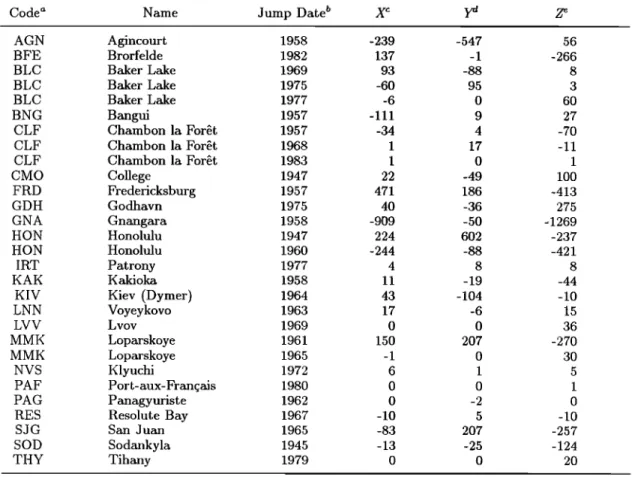
detected, we carefully checked the consistency of the monthly mean values with the annual mean values on

the same CD-ROM (labeled NGDC 05/1) by computing

the annual means from the monthly means and compar-

ing them with the archived values. This revealed that

in some observatories and at certain epochs changes in the base level had been applied to the annual means

(indicated

by "J" in the file called "annual"

on NGDC

for this, by simply applying the required changes to the monthly series. When this correction did not give sat-

isfying results, more information was directly requested

from the observatories; several of them acknowledged that corrections due to changes in instrumental base-

lines had been omitted.

The lists of available observatories with the torre-

sponding code, geographical coordinates, lengths of time series and baseline corrections are given in Tables 2a and 2b (note that further useful data might still be

obtained from other observatories). The geographical

distribution of these observatories is shown on Figure 3. Let us emphasize that the process of establishing sound time series in the way just described, however time consuming, is both an essential step to the fol- lowing analysis and a very efficient way of identifying possible problems within the observatory data.

Results

The same analysis procedure as the one used previ-

ously for the synthetic tests has been applied to the X

21,982 ALEXANDRESCU ET AL.' WAVELET ANALYSIS OF GEOMAGNETIC JERKS

Table 2b. Corrections Made to Observatory Baselines in This Study

Code a Name Jump Date b X c ya Z e

AGN Agincourt 1958 -239 -547 56 BFE Brorfelde 1982 137 -1 -266 BLC Baker Lake 1969 93 -88 8 BLC Baker Lake 1975 -60 95 3 BLC Baker Lake 1977 -6 0 60 BNG Bangui 1957 -111 9 27 CLF Chambon la Forat 1957 -34 4 -70 CLF Chambon la Forat 1968 1 17 -11 CLF Chambon la Forat 1983 1 0 1 CMO College 1947 22 -49 100 FRD Fredericksburg 1957 471 186 -413 G D H G o dhavn 1975 40 -36 275 GNA Gnangara 1958 -909 -50 - 1269 HON Honolulu 1947 224 602 -237 HON Honolulu 1960 -244 -88 -421 IRT Patrony 1977 4 8 8 K AK K akioka 1958 11 - 19 -44

KIV Kiev (Dymer) 1964 43 -104 -10

LNN Voyeykovo 1963 17 -6 15 LVV Lvov 1969 0 0 36 MMK Loparskoye 1961 150 207 -270 MMK Loparskoye 1965 - 1 0 30 NVS Klyuchi 1972 6 1 5 PAF Port-aux-Franqais 1980 0 0 1 PA G P an agyuris t e 1962 0 - 2 0

RES Resolute Bay 1967 -10 5 -10

SJG San Juan 1965 -83 207 -257

SO D S o dankyla 1945 - 13 - 25 - 124

THY Tihany 1979 0 0 20

'*According to the IAGA convention.

bAccording to Table 2a.

CCorrection applied to X component, in nanotesla.

el Correction applied to Y component, in nanotesla.

eCorrection applied to Z component, in nanotesla.

small number of observatories have long enough records

to allow

for the detection

of the jerks occurring

during

the first quarter of the century. The whole set of re- sults is given in Tables 3a-g; the dates found for the jerks cluster into seven groups hereinafter referred to as the 1901, 1913, 1925, 1932, 1949, 1969, and 1978 events

(Figure 4). For each of the seven jerks detected in the

data series, the extinction angle 0e can be determined with the same accuracy as in the case of the synthetic

tests.

0 ø 0 ø

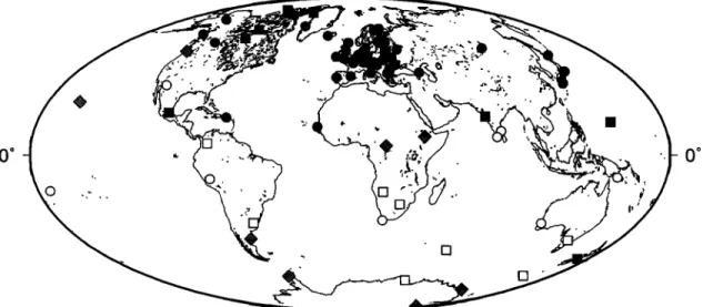
Figure 3. Distribution of the 97 observatories consid- ered in the present study. See also Table 2a for more

details.

Early Events

The 1901 event was successfully detected in all ob- servatories with available data for this epoch. It clearly

appears, with well-defined ridge functions of type 1, in three European observatories (CLF, COI, NGK, see Ta- ble 3a and Figure 5). It is also present, as a late edge

of an energy

packet

(see

the appendix

for more

details),

in the wavelet transforms of the HRB and KAK se-

ries. However, the insufficient duration of the records

for these two observatories (compare Table 2a) did not allow us to recover the ridge functions over a large range of dilations. Dates (1902.0+ 0.5) and regular-

Table 3a. Results for the 1901 Event

oa Ob b a • Dated Code

125 90 1.60 1901.33 CLF

120 70 1.66 1902.60 COI

130 80 1.55 1902.17 NGK aDirection angle of the jerk in degrees.

bEnhancement

angle

of the

jerk in degrees.

CSlope of the ridge function.

aDate

of occurrence

of the jerk.

ALEXANDRESCU ET AL.' WAVELET ANALYSIS OF GEOMAGNETIC JERKS 21,983

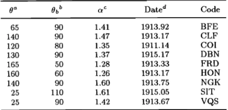
Table 3b. Results for the 1913 Event Table 3d. Results for the 1932 Event

0 a 0b b c•C Datea Code 0 a 0b • c• c Date a Code

65 90 1.41 1913.92 BFE 140 90 1.47 1913.17 CLF 120 80 1.35 1911.14 COl 130 90 1.37 1915.17 DBN 165 50 1.28 1913.33 FRD 160 60 1.26 1913.17 HON 140 90 1.60 1913.75 NGK 25 110 1.61 1915.05 SIT 25 90 1.42 1913.67 VQS

•Direction angle of the jerk in degrees.

bEnhancement angle of the jerk in degrees.

•Slope of the ridge function.

UDate of occurrence of the jerk.

ities (c• = 1.60 q-0.04) found for this jerk are almost

identical for the three observatories where they could be computed. It seems safe to conclude that the 1901 jerk is observed in a large part of the northern hemi- sphere, but it may be of worldwide extent.

The 1913 event has also been detected in all observa-

tories with sufficient data (see Table 2a). It is clearly ob- served in five European (BFE, CLF, COI, DBN, NGK) and three North American (FRD, SIT, VQS) observa- tories and HON (Table 3b and Figure 6). Most dates of this jerk cluster at the average date (1913.6q- 1.1). However, the dates of the event at COI and DBN are

surprisingly far from the average. The regularities esti-

mated from the nine ridge functions (Figure 6) give an

average of 1.42 q- 0.12. This event again could very well

be worldwide.

The 1925 event is clearly observed at five European

observatories (BFE, CLF, DBN, ESK, NGK) and two North American ones (TUC and SIT), but not at FRD

(Table 3c and Figure 7). This jerk has also been de-

tected for the remaining observatories EBR and SOD

(with less data) as an energy packet in the wavelet

transform. The average date and regularity are 1925.2q- 0.8 and 1.64q-0.19, respectively. This event could again

be worldwide.

The 1932 event does not show up everywhere. It is

detected at the FRD and HON observatories and in the

Table 3c. Results for the 1925 Event

0 • 0• • c• • Date a Code 60 80 1.48 1925.08 BFE 55 80 1.67 1924.08 CLF 50 50 1.84 1924.25 DBN 45 80 1.90 1926.42 ESK 55 80 1.52 1925.50 NGK 50 110 1.33 1925.52 SIT 115 90 1.73 1925.50 TUC 85 110 1.92 1932.08 45 90 1.55 1931.75 10 50 1.57 1932.00 25 80 1.60 1930.58 60 80 1.65 1933.83 50 80 1.46 1934.08 AML API FRD GNA HON HUA

•Direction angle of the jerk in degrees.

t'Enhancement angle of the jerk in degrees.

•Slope of the ridge function.

aDate of occurrence of the jerk.

southern hemisphere at the four observatories (AML, API, GNA and HUA) whose time series are long enough to allow for such a detection (Table 3d and Figure 8).

The averaõe date and reõularity found for this jerk are 1932.4 q- 1.2 and 1.63 q- 0.14, respectively. This event is

not seen in any of the European observatories.

The 1949 event is again not seen in Europe. It is

observed in the Pacific area (ABG, AML, API, GNA, KAK) and in the American region (FRD, HON, HUA, SJG, TUC) (Table 3e and Figure 9). The average date

and regularity estimated for this event are 1949.8 q- 1.4 and 1.49 q- 0.27, respectively. The 1949 jerk covers the same geographical area as the 1932 event. We will not discuss any further those early events which are much less documented than the 1969 and 1978 ones, on which

we will now focus.

The 1969 and 1978 Events

The worldwide character of the 1969 event is attested

by its presence in a large number of observatories dis-

tributed all around the world (at 66 observatories out of the 74 covering the time span around the event (Ta- ble 2a)). The ridge functions of this jerk are very clear

for 47 observatories where they are linear over a large

dilation range (Table 3f and Figure 10). We note evi-

dence of this jerk in the form of conelike energy patches

in the wavelet transforms of the series at 19 other oh-

Table 3e. Results for the 1949 Event

b 0 • Ob Date a Code 30 80 1.78 1947.67 ABG 75 80 1.36 1949.08 AML 30 70 1.00 1949.25 API 170 50 1.64 1950.00 FRD 120 100 1.63 1949.83 GNA 165 60 1.39 1950.83 HON 115 170 1.44 1951.58 HUA 120 100 1.13 1949.67 KAK 170 40 1.83 1952.42 SJG 155 100 1.74 1947.83 TUC aDirection angle of the jerk in degrees.

bEnhancement angle of the jerk in degrees.

•Slope of the ridge function.

UDate of occurrence of the jerk.

•Direction angle of the jerk in degrees. bEnhancement angle of the jerk in degrees.

•Slope of the ridge function.

21,984 ALEXANDRESCU ET AL.' WAVELET ANALYSIS OF GEOMAGNETIC JERKS

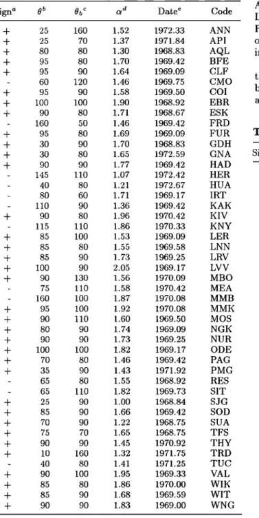
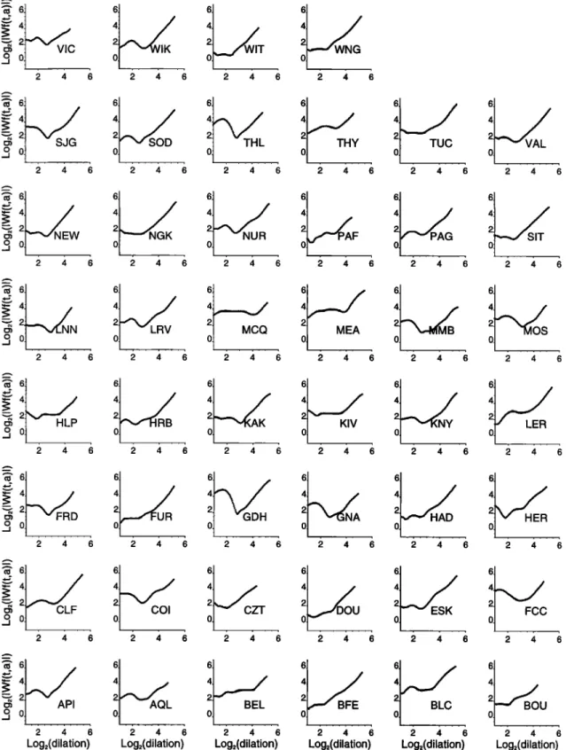
Table 3L Results for the 1969 Event

Sign a 0 b Ob c o•d Date • Code

+ 25 160 1.52 1972.33 ANN + 25 70 1.37 1971.84 API + 80 80 1.30 1968.83 AQL + 95 80 1.70 1969.42 BFE + 95 90 1.64 1969.09 CLF - 60 120 1.46 1969.75 CMO + 95 90 1.58 1969.50 COl + 100 100 1.90 1968.92 EBR + 90 80 1.71 1968.67 ESK - 160 50 1.46 1969.42 FRD + 95 80 1.69 1969.09 FUR + 30 90 1.70 1968.83 GDH + 30 80 1.65 1972.59 GNA + 90 90 1.77 1969.42 HAD - 145 110 1.07 1972.42 HER - 40 80 1.21 1972.67 HUA - 80 60 1.71 1969.17 IRT - 110 90 1.36 1969.42 KAK + 90 80 1.96 1970.42 KIV - 115 110 1.86 1970.33 KNY + 85 100 1.53 1969.09 LER + 85 80 1.55 1969.58 LNN + 85 90 1.73 1969.25 LRV + 100 90 2.05 1969.17 LVV + 90 130 1.56 1970.09 MBO - 75 110 1.58 1970.42 MEA - 160 100 1.87 1970.08 MMB + 95 100 1.92 1970.08 MMK + 90 110 1.60 1969.50 MOS + 80 90 1.74 1969.09 N G K + 90 90 1.73 1969.25 NUR + 100 100 1.82 1969.17 ODE + 70 80 1.46 1969.42 PAG + 35 90 1.43 1971.92 PMG - 65 80 1.55 1968.92 RES - 65 110 1.82 1969.73 SIT + 25 90 1.00 1968.84 SJG + 85 90 1.66 1969.42 SOD + 70 90 1.22 1968.75 SUA + 75 70 1.65 1968.75 TFS + 90 90 1.45 1970.92 THY + 10 160 1.32 1971.75 TRD - 40 80 1.41 1971.25 TUC + 90 100 1.95 1969.33 VAL + 85 80 1.86 1970.00 WIK + 85 90 1.68 1969.59 WIT + 90 90 1.83 1969.00 WNG

aThe sign of jerk detected fi'om the wavelet maps.

bDirection angle of the jerk in degrees.

CEnhancement angle of the jerk in degrees.

dSlope of the ridge function.

•Date of occurrence of the jerk.

servatories (despite their limited records), distributed worldwide (ABG, AML, BLC, DOU, FCC, FUQ, GUA, HBK, HRB, LAS, MAW, MBC, MCQ, MNK, PAF, TEO, THL, TOO, TSU).

The 1978 event displays the same global character,

being visible at 71 observatories out of 78. It is detected

and shows clear ridge function signatures in 46 observa-

tories, distributed worldwide (Table 3g and Figure 11).

For 25 other observatories the event is located close to

the beginning or the end of the available series (ABG,

ANN, BNG, BRW, DRV, FUQ, HBK, HYD, IRT, KOD, LAS, MBC, MBO, MNK, NVS, PMG, POD, PPT,

RES, SAB, SUA, TFS, TRD, TRW, TSU). For all these

observatories the event is detected from energy patches

in the wavelet transforms.

A very interesting feature revealed by this analysis is that the distribution of the dates of occurrence is clearly

bimodal (Figure 12) for both events. For the 1969 event

a first group of dates is centered on 1969.4+0.5 and an-

Table 3g. Results for the 1978 Event

Sign • 0 b Ob • a • Date • Code

- 40 80 1.88 1978.25 API - 90 80 1.05 1978.00 AQL - 90 80 1.29 1978.00 BEL - 60 80 1.46 1978.09 BFE + 50 90 1.60 1978.17 BLC -1- 45 100 1.38 1978.67 BOU - 60 80 1.89 1978.59 CLF - 40 100 1.01 1977.67 COl - 45 80 1.09 1981.75 CZT - 40 80 1.53 1978.00 DOU - 40 80 1.37 1977.59 ESK + 65 100 1.73 1977.92 FCC + 45 70 1.64 1978.09 FRD - 40 80 1.83 1978.00 FUR - 160 50 1.81 1976.84 GDH + 25 90 1.78 1980.92 GNA - 45 90 1.64 1978.09 HAD - 45 90 1.36 1982.00 HER - 85 90 1.50 1980.80 HLP - 90 80 1.79 1978.50 HRB + 145 110 1.63 1977.84 KAK - 70 70 1.51 1977.75 KIV + 155 100 1.85 1979.33 KNY - 45 80 1.67 1977.92 LER - 50 90 1.42 1977.58 LRV - 100 70 1.97 1976.42 LNN - 65 120 1.28 1978.00 MCQ + 75 110 i.78 1976.67 MEA + 155 100 1.52 1977.83 MMB - 110 40 1.89 1976.50 MOS + 65 90 1.95 1978.37 NEW - 50 80 1.69 1978.17 NGK - 40 90 1.40 1977.67 NUR + 50 70 1.58 1981.92 PAF - 35 90 1.51 1977.75 PAG + 50 100 1.58 1977.71 SIT + 55 70 1.72 1977.92 SJG - 25 80 1.65 1978.09 SOD - 10 40 1.63 1976.67 THL - 60 90 1.44 1977.67 THY + 50 80 1.66 1978.00 TUC - 45 90 1.74 1978.25 VAL + 60 80 1.76 1977.58 VIC - 40 80 1.83 1979.00 WIK - 25 80 1.78 1978.17 WIT - 45 80 1.65 1978.25 WNG

•The sign of jerk detected from the wavelet maps.

bDirection angle of the jerk in degrees.

CEnhancement angle of the jerk in degrees.

aSlope of the ridge function.

ALEXANDRESCU ET AL.' WAVELET ANALYSIS OF GEOMAGNETIC JERKS 21,985

o

19oo

,[ I I ,,,,, ,,u,

, , , , , i , , , , ! , , , , i , , , , i ,

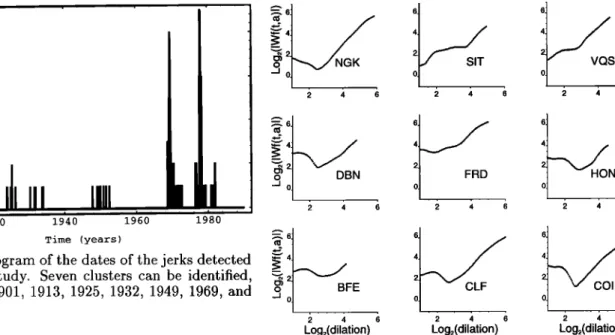
Time (years)

Figure 4. Histogram of the dates of the jerks detected

in the present study. Seven clusters can be identified,

roughly dated 1901, 1913, 1925, 1932, 1949, 1969, and

1978.

other one on 1972.1 4-0.5. In a similar way, the dates

of the 1978 event split into a first group centered

on

Figure

13, which

shows

the geographical

distribution

of the dates of occurrence, further reveals that the hi-

modal

temporal

distribution

of the 1969

jerk is also

as-

sociated

with a clear geographical

pattern: the jerk ap-

pears

at a later

date

in the southern

hemisphere.

This

result is corroborated by the analysis of the wavelet

maps

of eight

other

observatories

located

in the south-

ern hemisphere

(FUQ, HBK, LAS, MAW, MCQ, PAF,

TOO, and TSU) and for which

the examination

of the

energy

packet

also

suggests

a date around

1972. Fig-

ure 14 shows that exactly the same thing happens to be true for the 1978 event. The occurrence time is

again

later

in the southern

than

in the northern

hemi-

sphere

with a similar

time lag of about 2 to 3 years

(note,

however,

that the number

of analyzed

southern

series is even smaller than for the 1969 event). Again

also,

this later date is confirmed

by inspecting

the cone-

like energy

patches

typical

of jerks

within

the wavelet

maps of 12 additional

observatories

with shorter

se-

ries

(ABG,

ANN, DRV,

FUQ, HBK, HYD, KOD, LAS,

PMG, PPT, TRW, and TSU). Thus

the two 1969

and

1978 events seem to share a common spario-temporal

behavior.

To what extent can this similarity be generalized to

the regularity

c• and the local

direction

0, both param-

o CLF K

ß ,

2 4 6 2 4 6 2 4

Log2(dilation) Log2(dilation) Log•(dilation)

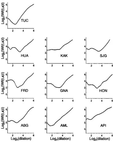
Figure 5. Log-log

plots of the ridge

functions

of the

1901

event

(see

Table

2a for the code

and

location

of the

observatories and Table 3a for ridge function slopes).

2 4 6 2 4 6 2 4 o • FRD N 2 4 6 2 4 6 2 4 6

61

6

6

•o•

ø

E

0

Figure 6. Log-log

plots of the ridge functions

of the

1913

event

(see

Table 2a for the code

and location

of the

eters being available at 47 observatories for the 1969 event, and 46 observatories for the 1978 event? We

note that the average values of the o• for 1969 and 1978

events happen to be equal (c• - 1.6). But we also note that within each event, the measured values of c• vary significantly from place to place (Tables 3f and 3g).

We measured this dispersion in terms of a global stan- dard deviation with respect to the previous average val- ues. Again we found exactly the same value era = 0.23 for both events. This value is slightly larger than the

standard deviation we expected from our s•n•.•z• test

2 4 6 ,•,6 6 6 v o, ESK ß . 2 4 6 2 4 6 2 4 6 2 4 6 2 4 6 2 4 6

Log2(dilation) Log•(dilation) Log•(dilation)

Figure 7. Log-log

plots of the ridge

functions

of the

1925

event

(see

Table

2a for the code

and

location

of the