O
pen
A
rchive
T
OULOUSE
A
rchive
O
uverte (
OATAO
)
OATAO is an open access repository that collects the work of Toulouse researchers and makes it freely available over the web where possible.
This is an author-deposited version published in : http://oatao.univ-toulouse.fr/
Eprints ID : 15868
To link to this article : DOI:10.1017/jfm.2015.338 URL : http://dx.doi.org/10.1017/jfm.2015.338
To cite this version : Alméras, Elise and Risso, Frédéric and Roig, Véronique and Cazin, Sébastien and Plais, Cécile and Augier, Frédéric Mixing by bubble-induced turbulence. (2015) Journal of Fluid
Mechanics, vol. 776. pp. 458-474. ISSN 0022-1120
Any correspondence concerning this service should be sent to the repository administrator: [email protected]
Mixing by bubble-induced turbulence
Elise Alméras1,2, Frédéric Risso1,†, Véronique Roig1, Sébastien Cazin1,
Cécile Plais2 and Frédéric Augier2
1Institut de Mécanique des Fluides de Toulouse, Université de Toulouse and CNRS, Allée C. Soula,
31400 Toulouse, France
2IFP Energies nouvelles, Rond-point de l’échangeur de Solaize, BP 3, 69360 Solaize, France
This work reports an experimental investigation of the dispersion of a low-diffusive dye within a homogeneous swarm of high-Reynolds-number rising bubbles at gas volume fractions ↵ ranging from 1 % to 13 %. The capture and transport of dye within bubble wakes is found to be negligible and the mixing turns out to result from the bubble-induced turbulence. It is described well by a regular diffusion process. The diffusion coefficient corresponding to the vertical direction is larger than that corresponding to the horizontal direction, owing to the larger intensity of the liquid fluctuations in the vertical direction. Two regimes of diffusion have been identified. At low gas volume fraction, the diffusion time scale is given by the correlation time of the bubble-induced turbulence and the diffusion coefficients increase roughly as ↵0.4.
At large gas volume fraction, the diffusion time scale is imposed by the time interval between two bubbles and the diffusion coefficients become almost independent of ↵. The transition between the two regimes occurs sooner in the horizontal direction (1 %6 ↵ 6 3 %) than in the vertical direction (3 % 6 ↵ 6 6 %). Physical models based on the hydrodynamic properties of the bubble swarm are introduced and guidelines for practical applications are suggested.
Key words: bubble dynamics, gas/liquid flow, mixing and dispersion
1. Introduction
Bubbly flows are used in many industrial applications to favour contact between a gas and a liquid in view of enhancing mass transfer and chemical reactions. Bubble columns are particularly interesting because the rising motion of the bubbles generates liquid fluctuations which mix the chemical species without requiring any additional mechanical agitation. Up to now, the design of such systems has been based on the use of an empirical turbulent Schmidt number (see Radl & Khinast
2010, and references therein). The dispersion of a solute is described by an effective diffusion with a diffusion coefficient that is chosen to be proportional to the turbulent eddy viscosity through an empirical prefactor. The prefactor is found to depend on many parameters, such as the turbulent intensity, the gas volume fraction or the
column geometry. In the absence of any reliable theory, it is generally arbitrarily tuned between 0.1 and 2.2 to provide realistic results (Combest, Ramachandran & Dudukovic 2011).
The modelling of the mixing in a bubbly flow requires first knowledge of the hydrodynamic characteristics of the agitation within the liquid, and then an understanding of the properties of dispersion of this agitation. Concerning liquid dynamics, it is now well established that bubble-induced agitation has features that make it different from shear-induced turbulence. A series of experimental investigations carried out in homogeneous columns have led to a rather complete description of its properties (Martínez-Mercado, Palacios-Morales & Zenit 2007; Martínez-Mercado et al. 2010; Riboux, Risso & Legendre 2010; Mendez-Diaz, Serrano-García & Zenit 2013). On the other hand, no fundamental investigation of bubble-induced mixing has been performed so far, except for the preliminary work of Mareuge & Lance (1995), which was limited to a single very small value of the gas volume fraction, ↵ = 0.2 %.
The objective of this study is to determine the characteristics of the mixing induced by bubbles in the absence of any liquid mean flow and shear-induced turbulence. For that purpose, we have measured the dispersion of a volume of dye injected within a swarm of air bubbles rising in water. For the considered range of gas volume fractions (16 ↵ 6 13 %) and bubble Reynolds number (⇡700), the bubble-induced turbulence is well developed while the swarm remains stable and homogeneous. Since the dye has a low concentration and a very low molecular diffusion (Schmidt number of 2500) we can consider it to be a passive scalar transported by the flow. Our motivation is to understand the physical mechanisms underlying the mixing. Previous results obtained in a two-dimensional bubble column where bubble-induced turbulence cannot develop have shown that the capture and the transport of a solute within the bubble wakes cannot be described by an effective diffusion (Bouche et al.2013). First, it is therefore important to settle the question of whether it is a diffusion process or not in a three-dimensional bubble column. Then, it is desirable to relate the mixing properties to the time, length and velocity scales of the bubble swarm in order to propose models.
The paper is organized as follows. Section 2 describes the experimental set-up and the measuring methods, while §3 recalls the hydrodynamic characteristics of the bubble swarm. Section 4 presents experimental results concerning the mixing, which are then interpreted and modelled in §5. Guidelines for applications and further work are discussed in §6.
2. Experimental set-up and instrumentation
The experimental set-up is depicted in figure 1. The test section is an open tank made of glass 1000 mm in height, with a rectangular cross-section of 150 mm ⇥ 300 mm. It is filled with tap water and air bubbles are continuously injected at the bottom through 1800 capillary tubes of 0.2 mm inner diameter, which are distributed on a regular array with a spacing of 5 mm. The gas volume fraction ↵ is varied from 1 % to 13 % by adjusting the inlet gas flow rate. In this range a homogeneous swarm of rising bubbles is generated and no coalescence takes place.
The characteristics of the gas phase are determined by means of a dual optical fibre probe from RBI, which detects the passages of the bubble interfaces at two points separated by a distance of 2.15 mm in the vertical direction. The signal processing is not detailed here since it has already been described in Riboux et al. (2010) and Colombet et al. (2011). Bubble sizes and gas volume fraction are estimated from the
Dye injector
Air injectors
Front view Top view
1000 mm UV neons 300 mm 300 mm 150 mm Bandpass filter (450–650 nm) Camera z x z x 7 6 5 4 3 2 1 8 9 10 11 12
FIGURE 1. Experimental set-up.
time periods at which the leading probe passes within each bubble. Bubble velocities are measured from the intervals between the instants a bubble successively touches the two probes. The technique has been validated by comparison with image processing. The resulting accuracy is better than 2 % for the gas volume fraction ↵, 5 % for the average bubble velocity V, and 10 % for the average bubble equivalent diameter d.
Mixing experiments consist in measuring the evolution of a patch of dye within the bubble swarm. The dye is fluorescein sodium, which has a molecular diffusion coefficient in water, Dm= 4 ⇥ 10 10 m2 s 1 at 22 C, much smaller than the water
kinematic viscosity ⌫, and a high Schmidt number, Sc = ⌫/Dm= 2500. An aqueous
solution of fluorescein sodium at concentration C0 = 5 ⇥ 10 3 mol l 1 is injected
within the bubble swarm through a vertical tube of 0.5 mm inner diameter and 0.9 mm outer diameter. The tube is inserted from the top of the tank in the middle of the cross-section. The dye injection point is located 500 mm above the gas injectors in order to ensure that the dye does not interact with either the top or the bottom of the tank during an experiment. At the beginning of each run, 1 ml of dye solution is injected during 2 s at a constant flow rate of 30 ml min 1 by
means of a volumetric pump. This makes a turbulent jet with a Reynolds number of approximately 1300, which interacts with the bubbles. At the end of the injection a grossly ellipsoidal patch of dye approximately 100 mm in height and 50 mm in width is formed. Ten seconds after the beginning of the injection, the initial conditions are forgotten and the evolution of the dye is totally controlled by the bubble-induced agitation. The beginning of the injection is chosen as the origin of time and quantitative measurements are considered only for times larger than 10 s.
The dye concentration is measured by means of induced fluorescence. Twelve vertical ultraviolet neon tubes are arranged around the tank in order to generate a
300 400 500 600 700 800 900 0
0.5 1.0 1.5
Power spectral density
Dye absorption Dye emission Neon light Camera range
FIGURE 2. Spectrum of UV-neon light, fluorescein absorption and emission spectra, and range of wavelengths collected by the camera.
homogeneous lighting of the flow. The spectrum of the light emitted by the present neon tubes has been measured by means of a USB2000+ spectrometer from Ocean Optics. Figure 2 shows that it falls mainly within the range of wavelengths from 350 and 400 nm. The fluorescein sodium is a fluorescent dye that absorbs light in the range of wavelengths from 350 to 550 nm (peak at 500 nm) and emits light in the range from 480 to 640 nm (peak at 520 nm). A PCO EDGE sCMOS digital camera (2560 pixels ⇥ 2160 pixels, 16 bits) equipped with an 85 mm optical lens with an aperture f /D = 2.8 is used to film a field 345 mm in width and 410 mm in height centred around the dye injection point. The depth of field is much larger than the test section and the variation of magnification throughout the imaged volume of flow is negligible, with a pixel size of 0.16 mm. The camera takes 49 images per second with an exposure time of 10 ms. An optical bandpass filter (450–650 nm) is mounted in front of the camera in order to remove the neon light and ensure that only the light that is fluoresced by the dye is collected. Under appropriate conditions, the light intensity collected by each pixel, and thus its grey level, is proportional to the mass of dye in the volume of fluid imaged by the corresponding pixel.
Before investigating the mixing, two groups of preliminary experiments have been conducted by imaging a hollow transparent plastic sphere of 50 mm diameter filled with an aqueous solution of fluorescein sodium of known concentration.
In the first group of preliminary experiments, tests were conducted in the absence of bubbles in order to define a suitable concentration of dye and calibrate the method. First, the centre of the sphere is located at the dye injection point and various concentrations are considered. For CS= 5 ⇥ 10 6 or 5 ⇥ 10 5 mol l 1 (figure 3a), the
grey level of each pixel is found to be proportional to the dimension of the sphere in the direction of view. For CS= 5 ⇥ 10 4 or 5 ⇥ 10 3 mol l 1 (not displayed here),
the mass of dye is so large that absorption is no longer negligible and saturation of the fluorescence signal occurs near the centre of the sphere. In a second step, the concentration is fixed to CS= 5 ⇥ 10 5 mol l 1 and the intensity of the lighting is
(a) (b)
(d ) (c)
FIGURE 3. (Colour online) Steps of the image processing technique applied to a sphere that is filled with dye at concentration CS= 5 ⇥ 10 5 mol l 1: (a) reference image in the absence of bubbles; (b) raw image within the bubble swarm at ↵ = 3.9 %; (c) image obtained after taking the minimum and detected contour; (d) final result of the procedure.
changed by progressively decreasing the number Nt of neon tubes that are switched
on (see figure 1): Nt= 12 (all tubes), Nt= 8 (tubes nos. 1, 2, 4, 6, 7, 9, 11 and 12),
Nt = 6 (tubes nos. 1, 3, 6, 7, 10 and 12), Nt= 4 (tubes nos. 1, 6, 7 and 12). As
expected, the grey levels are found to be proportional to the number of activated neon tubes. Third, with all the neon tubes being switched on and CS= 5 ⇥ 10 5 mol l 1,
the sphere centre is moved to different locations. No variation of the grey-level profiles is observed, which confirms that the lighting is homogeneous throughout the test section and there is no optical distortion. To sum up, in the present set-up, provided the dye concentration is not higher than 5 ⇥ 10 5 mol l 1 in a volume
of fluid of 50 mm dimension in the y-direction, the fluorescence lies in the linear regime regarding both the lighting intensity and the dye concentration. In the absence of bubbles, the grey level measured in each camera pixel is therefore proportional to the mass of dye.
In the second group of preliminary experiments, tests have been conducted with the sphere immersed in the bubble swarm in order to assess optical distortion due to bubbles and eliminate them. As visible in figure 3(b), the presence of the bubbles strongly affects the image. Two major effects can been identified. First, a fraction of the fluoresced light emitted by the sphere that is not initially directed towards the camera is reflected or refracted in the direction of the camera by the bubbles that surround the sphere. Instead of being totally dark, the vicinity of the sphere thus appears brighter. The contour of the sphere, which appears very sharp and easy to detect in figure 3(a), therefore spreads out over a significant distance in figure 3(b). Secondly, the bubbles that are located between the sphere and the camera hide a fraction of the fluoresced light that should reach the camera. The image of the sphere is thus darker that it should be.
1.2 1.0 0.8 0.6 0.4 0.2 0 0 1.2 1.0 0.8 0.6 0.4 0.2 0 –5 5 –5 0 5 Normalized prof iles (a) (b)
FIGURE 4. Grey-level profiles passing through the sphere centre: (a) raw image; (b) after image processing.
A two-step procedure has been developed to correct these two effects. The vertical distance travelled by each bubble between two successive images is approximately 6 mm (⇡2d). The locations of the light spots generated by bubble refraction and reflection are thus totally different from one image to another. Considering 15 successive images, there is at least one image in which no light spot is present in each given pixel located outside the sphere. The darker a pixel, the lower the grey level. Taking the minimum of the grey levels of each pixel over 15 successive images allows one to set the exterior of the sphere at the level of the background noise (see figure 3c). It is easy to detect the contour of the sphere by simple thresholding of the minimum image. The spreading of the region containing the dye is then removed by turning to black all the pixels of the original image that are located outside the contour. While the threshold has been adjusted to each gas volume fraction according to the maximum of intensity within the minimum image, the results were found to be weakly sensitive to that threshold. Considering again 15 successive images, there is at least one image in which the fluoresced light directed towards each pixel imaging the sphere is not intercepted by any bubble. Taking the maximum grey level of each pixel over 15 successive images hence allows one to cancel the darkening of the interior of the sphere. The image resulting from application of the whole procedure, shown in figure 3(d), compares well with the image taken in the absence of bubbles (figure 3a). Finally, the horizontal (resp. vertical) profiles are obtained by taking the maximum of the grey levels over 21 lines of pixels located at z (resp. x) ±10 pixels around the sphere centre. Figure 4 shows the horizontal profiles of grey level before and after image processing for ↵ = 3.9 and 10.5 %. A good agreement with the reference case without bubbles (↵ = 0) is again obtained.
The previous procedure having been validated for a volume of dye of known geometry and concentration, it is then applied to a patch of dye injected within the bubble swarm. The only difference from the preliminary tests done using a sphere is that bubbles are now present within the dye region. Supplementary tests using backlighting (detailed in Alméras 2014) have shown that bubbles immersed in a
0 5 10 0 0.5 1.0 1.5 2.0 Grey-level profile Raw image Treated image –10 –5 (a) (b) (c)
FIGURE 5. (Colour online) Illustration of image processing applied to mixing experiments (t = 10 s, ↵ = 3 %): (a) raw image with detected contour; (b) image after processing; (c) horizontal profiles of grey levels before and after treatment.
solution of homogeneous dye concentration never induce local values greater than in the absence of bubbles and only cause an additional light occultation. Therefore, taking the maximum of grey levels allows one to detect instants when no bubbles, neither inside nor outside the patch, are visible by a given pixel. We are thus confident that the image treatment is still valid.
Figure 5(a) shows an example of a raw image of the patch of dye (t = 10 s, ↵ = 3 %), whereas figure 5(b) shows the same image after processing. Figure 5(c) compares the corresponding horizontal profiles of the grey levels before and after treatment.
Note that the dye concentration at injection is fixed at C0= 5 ⇥ 10 3 mol l 1 for all
mixing experiments. Depending on the gas volume fraction, the volume of the patch of dye reaches a size which is two orders of magnitude (⇡100 ml) larger than the injected volume (1 ml) between 2 and 10 s. This dimension is of the order of that of the sphere used in preliminary tests and its average concentration is approximately 5 ⇥ 10 5 mol l 1, which is the maximal value below which fluorescence is not limited
by light absorption by the dye. We have chosen the largest initial concentration, ensuring that grey levels are actually proportional to the mass of dye, in order to maximize the intensity of the fluoresced light, and consequently optimize the signal-to-noise ratio. Practically, this choice allows us to obtain reliable measurements during a time interval of 15 s until the average dye concentration is greater than 5 ⇥ 10 7 mol l 1. At larger gas volume fractions, this time interval starts at t = 10 s
and ends at t = 25 s, while at lower volume fractions it ranges from t = 20 s to t = 35 s.
We have thus developed a measurement technique that allows us to investigate the mixing of a patch of low-diffusive dye within a homogeneous swarm of bubbles during 15 s, for gas volume fractions from 1 % to 13 %. The spatial resolution is 21 pixels (3.36 mm), which is 10 times larger than the length scale LD of the
molecular diffusion over the duration Te of an experiment (LD=pDmTe⇡ 0.2 mm for
Te= 10 s). While the camera grabbing rate is 49 Hz, each concentration measurement
makes use of 15 consecutive images, so that the effective time resolution is 0.3 s.
3. Hydrodynamic characteristics of the bubble swarm
The dynamics of both phases has already been experimentally investigated in detail (Riboux et al. 2010; Colombet et al. 2011, 2014) and also numerically simulated (Riboux, Legendre & Risso 2013). In particular, the present bubble injection uses the same capillary tubes with the same spatial distribution as in previous experiments mentioned above. The only difference from the former set-up is that the tank cross-section is a rectangle of 15 cm ⇥ 30 cm instead of a square of 15 cm ⇥ 15 cm, a wider system being required to allow a sufficient time before the dye reaches the walls. For a homogeneous flow, the size of the tank is not a control parameter. An extensive investigation of the dynamics has therefore not been carried out again in the present work.
The main characteristics of the gas phase have been measured in the present set-up. They confirm that the flow configuration is actually the same as in previous experiments. Various profiles of ↵ have been measured to check that the gas injection is uniform and that the flow corresponds to a stable bubble column without large-scale recirculations. As ↵ is increased from 1 % to 13 %, the bubble equivalent diameter d increases from 2.3 to 3.9 mm, whereas the average bubble rise velocity V decreases from 300 to 215 mm s 1, values which correspond to mobile interfaces and indicate
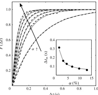
that there is no significant effect of surface-active contaminants. Consequently, the bubble Reynolds number, Re = Vd/⌫, remains within the narrow range 680–840. The spatial distribution of the bubbles has been assessed by considering the statistics of the time intervals between the arrivals of two successive bubbles on the leading optical probe. Figure6 shows the distribution function F(1t), which is the probability that the time intervals t are smaller than 1t. If the bubble locations are statistically independent of each other, the process should be Poissonian:
F(1t) = Prob( t < 1t) = 1 exp( 1t/1tm). (3.1)
The theoretical expression (3.1) has been fitted to experimental data by adjusting the average time interval 1tm and found to be in good agreement with the measurements,
except for slight differences at large volume fractions. We can conclude that bubble locations can be considered as statistically independent and there is no bubble clustering, which extends the results obtained at lower volume fractions by Risso & Ellingsen (2002). Assuming that bubbles are oblate ellipsoids of aspect ratio , rising at velocity V with their minor axis oriented vertically, the average time interval should be written as
1tm= 2d
3 2/3↵V. (3.2)
The inset in figure 6 compares the measured values of 1tm with expression (3.2),
where d and V are measured values for the corresponding volume fraction, and = 1.7 from Riboux et al. (2010). Equation (3.2) gives an accurate estimation of the average time interval between consecutive bubbles, which therefore scales as ↵ 1.
0 0.2 0.4 0.6 0.8 1.0 0.2 0.4 0.6 0.8 1.0 0 5 10 15 0.1 0.2 0.3 0.4
FIGURE 6. Time interval between consecutive bubbles for ↵ = 1.3 %, 3.0 %, 4.5 %, 6.8 %, 9.8 % and 13 %. Distribution function in the main figure and average time interval in the inset. Dark dashed-line or symbols: experimental measurements. Light continuous lines: (3.1) for F(1t) and (3.2) for 1tm.
The properties of the liquid agitation are known from Riboux et al. (2010). In the range of gas volume fraction considered here, the standard deviations of the horizontal and vertical fluctuations in the liquid are described well by the following empirical relations
u0
x= xV0↵0.4 with x⇡ 0.76, (3.3)
u0
z= zV0↵0.4 with z⇡ 1.14, (3.4)
where V0 = 320 mm s 1 is the rise velocity of an isolated bubble of d = 2.1 mm.
When normalized by the variance, the spatial spectra of the liquid fluctuations are independent of the gas volume fraction and similar in the horizontal and vertical directions. In particular, the Eulerian integral length scale ⇤ is found to be equal to 7.7 mm for all values of ↵ investigated and a k 3 subrange is observed for the scales
between ⇤/10 and ⇤.
4. Mixing induced by the bubbles
Figure 7 presents a typical evolution of the patch of dye for ↵ = 4.5 %. The first column shows pictures of the dye distribution after image processing at t = 5, 10, 15 and 20 s. The second column shows the horizontal and vertical grey-level profiles passing through the patch barycentre, which is chosen as origin of the coordinates. The patch is rather regular and symmetric relative to its centre. The symmetry in the horizontal direction just results from the homogeneity of the bubble swarm and the isotropy of the bubble-induced agitation in the horizontal plane. More interesting is the symmetry in the vertical direction, as it means that the upward flux of dye is equal to the downward flux of dye. The mechanism of transport by capture of dye within the bubble wakes, which should break the up/down symmetry, is therefore not dominant.
0 10 0 10 0 10 0 0.5 1.0 Grey levels 0 10 0 10 0 10 0 0.5 1.0 Grey levels 0 10 0 10 0 10 0 0.5 1.0 Grey levels 0 10 0 10 0 10 0 0.5 1.0 Grey levels –10 –10 –10 –10 –10 –10 –10 –10 –10 –10 –10 –10 (a) (b) (c) (d) (e) ( f ) (g) (h)
FIGURE 7. (Colour online) Time evolution of patch of dye for ↵ = 4.5 %: (a,b) t = 5 s; (c,d) t = 10 s; (e,f ) t = 15 s; (g,h) t = 20 s. (a,c,e,g) images; (b,d,f,h) experimental profiles of grey levels and curves fitted using (4.4).
Moreover, the grey-level profiles are approximately Gaussian. Altogether this suggests that the mixing could be described as a regular diffusion process.
Let us consider the evolution of the concentration Cfree of a mass M of dye
subjected to anisotropic diffusion in an unbounded domain. The solution of the diffusion equation in the principal frame of the diffusion tensor Dij reads (Socolofsky
& Jirka 2005): Cfree(x; y; z; t) = M (2p)3/2 x y zexp x2 2 2 x y2 2 2 y z2 2 2 z ! . (4.1) The variance 2
i of the Gaussian function in direction i is related to time by 2
i = 2Diit. (4.2)
Assuming that the diffusion is isotropic in a horizontal plane, we only introduce a horizontal and a vertical coefficient of diffusion: Dh=Dxx=Dyy and Dv=Dzz.
In the present configuration, the concentration is often not negligible at the walls, which are located at kxk = xw = 150 mm and kyk = yw = 75 mm. The equation of
diffusion being linear, its solution in a domain that is bounded by walls (no-flux condition) is obtained by summing an infinite number of mirror sources (Socolofsky & Jirka 2005): Cbd(x; y; z; t) = 1 X nx= 1 1 X ny= 1 Cfree(x + 2 nxxw; y + 2 nyyw; z; t). (4.3)
Since our experimental technique gives us access only to a two-dimensional view of the concentration field, Cbd cannot be directly compared with the measurements. By
integration of (4.3), we can however obtain a quantity that is proportional to the light collected by a camera pointing in the y-direction:
C2D(x; z; t) = Z yw yw Cbd(x; y; z; t) dy = M 2p x z 1 X nx= 1 exp ✓ (x + 2 nxxw)2 2 2 x z2 2 2 z ◆ . (4.4) It is interesting to note that, thanks to the properties of the exponential function, C2D is similar to the solution of a two-dimensional diffusion problem. Three sources
being largely sufficient to ensure a good accuracy, the infinite summation has been truncated to 16 nx 6 1. For each instant, the horizontal and vertical profiles of
grey level have been fitted with (4.4) by adjusting M, x and z by means of the
least-squares method. Figure 7 shows that the fitted profiles are in good agreement with the measured ones. The scattering of the measured profiles is at the noise level and should not be interpreted as the signature of turbulent eddies. The Gaussian fit can be considered only as an average distribution around which fluctuations, undetectable with the present technique, are expected to exist. The spatial resolution of the experimental method is 1x = 3.3 mm, which is approximately one half of the integral length scale ⇤ of the liquid-velocity fluctuations. The time resolution is 1t = 0.3 s, which is approximately a factor of three greater than the time for a bubble to travel over its diameter. The fact that the patch shape is observed to have converged towards a rather smooth Gaussian profile indicates that the mixing is mainly driven by eddies smaller than 1x, which have a turn-over time smaller than 1t. Larger eddies are expected to cause larger and larger striations as time increases. Corresponding striations are nevertheless not detectable, either in treated or raw images. This indicates that liquid fluctuations generated in a homogeneous bubble swarm do not involve eddies much larger than both its integral length scale or the bubble diameter. In the following we shall focus on the characteristics of the fitted Gaussian curve.
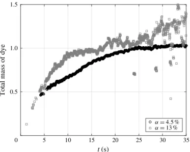
Figure 8 shows the time evolution of the measured value of M at ↵ = 4.5 % and 13 %. After the end of the injection, the total mass of dye within the tank is conserved. M should therefore be constant within the time interval where the experimental method has been validated (see §2). At ↵ = 4.5 %, the mixing has been investigated in the time interval from t = 20 s to t = 35 s. From t = 20 s to t = 25 s, M still increases by 5 % and then stabilizes within ±2.5 % from t = 25 s to t = 35 s. We checked that limiting the measurement period to the interval from t = 25 s to t = 35 s does not change the measured values of x and z. When increasing the gas volume fraction,
the accuracy in the determination of M decreases. In the harder case, at ↵ = 13 %, M experiences fluctuations within ±15 % during the measurement period which ranges from t = 10 s to t = 25 s. Again, limiting the measurement period to the range from t = 10 s to t = 15 s, where fluctuations are within ±5 %, has no significant effect on
10 15
5 20 25 30 35
Total mass of dye
0 0.5 1.0 1.5
FIGURE 8. Time evolution of the normalized mass M of dye for ↵ = 4.5 % and 13 %. Note that diffusion coefficients are measured during interval 10 s6 t 6 25 s for ↵ = 13 % and interval 20 s6 t 6 35 s for ↵ = 4.5 %, during which the measured mass is constant.
the measured values of x and z. We can therefore conclude that the value of M is
reasonably constant during the time interval over which the mixing is investigated and that its fluctuations have no significant influence on the measured values of x and z.
The measured total mass of dye is sensitive to fluctuations of the intensity of light that reaches the patch of dye, which may be affected by variations of the residual ambient light and by the number of bubbles that are present between the light source and the patch of dye. In contrast, the shape of the dye distribution is not sensitive to these fluctuations. The accuracy in the determination of x and z is therefore expected to
be much better than that of M. It is worth noting that the present method has been specially designed for the measurement of the evolution of the width of a patch of dye and must not be confused with classic methods based on laser-induced fluorescence, which aim at the determination of the absolute value of the concentration.
Figure 9 presents typical examples of time evolutions of the variances 2
x and z2
for ↵ = 9.8 %. The results of five independent tests are plotted (light-grey curves) as well as their average (black curve). For both directions, the reproducibility is good and the variance evolves linearly with time in the interval from t = 10 to 25 s. We also note that the slope is larger in the vertical direction than in the horizontal direction, indicating that the mixing is more efficient in the vertical direction. Similar results are obtained for all gas volume fractions from 1 % to 13 %. Since the spatial profile of the concentration is given by (4.4) and its temporal evolution by (4.2), we can conclude that the mixing process is described well by an anisotropic regular diffusion process. For each volume fraction, the average variance has been determined from five independent tests. The diffusion coefficients have then been obtained from the slope of the time evolution of the averaged curves and error bars estimated from the standard deviation of individual measurements. The symbols in figure 10 show the experimental diffusion coefficients in the horizontal and vertical directions, Dh and
Dv, as a function of the gas volume fraction, ↵. The values are within 1 to 6 cm2 s 1,
0.005 0.010 0.015 0.020 0.025 0.030 Measured slope 0.005 0.010 0.015 0.020 0.025 0.030 Measured slope 0 10 20 30 0 10 20 30 (a) (b)
FIGURE 9. (Colour online) Time evolution of the variance of the spatial distribution of the patch of dye for ↵ = 9.8 %. Light-grey curves, individual tests. Black curves, average over five tests.
0 2.5 5.0 7.5 10.0 12.5 15.0 1 2 3 4 5 6 7 8
FIGURE 10. Diffusion coefficients against gas volume fraction. Circles, measured horizontal coefficients (Dh). Squares, measured vertical coefficient (Dv). Dashed lines, model (5.1)–(5.2) for low ↵ with kl = 0.63. Continuous lines, model (5.3)–(5.4) for large ↵ with kh = 0.40. (Error bars correspond to the standard deviation of individual measurements.)
Dv is approximately three times larger than Dh for all ↵. As far as we know, the
only previous measurement of the diffusion of a low-diffusive passive scalar in a homogeneous swarm of bubbles (Mareuge & Lance 1995) was limited to a single very low value of the gas volume fraction: Dh= 0.4 cm2 s 1 and Dv= 0.7 cm2 s 1
for air bubbles of 5.8 mm equivalent diameter in water at ↵ = 0.2 %. The order of magnitude is comparable to the present one and the horizontal diffusion was also found to be lower than the vertical diffusion. However, we are not sure whether the bubble-induced turbulence can be considered as fully developed at such a small gas volume fraction.
We also see in figure 10 that the evolution of the diffusion coefficients against the gas volume fraction presents two different regimes. In the vertical direction, Dv
increases strongly with ↵, whereas its value becomes almost constant for ↵ larger than 6 %. In the horizontal direction, the increase of the diffusion coefficient from Dh= 0 at ↵ = 0 is here only described by the first measuring point at ↵ = 1.3 %.
A saturation is then observed for ↵ larger than 3 %. A comparable limitation of the horizontal diffusion coefficient when ↵ is increased beyond a few percent has already been observed by Abbas, Billet & Roig (2009) in a homogeneous bubble swarm where a horizontal gradient of dissolved oxygen developed owing to a difference in mass transfer resulting from a different composition of the gas mixture within the bubbles. Considering that hydrodynamics of the bubble swarm shows no transition and that the energy of the liquid fluctuations continuously increases in the considered range of ↵, the observed saturation of the diffusion coefficients was rather unexpected.
To understand the mechanisms underlying the mixing, we need to relate the characteristics of the dye diffusion to the hydrodynamics of the bubble swarm.
5. Physical interpretation and modelling
Two mechanisms are candidates to control the mixing of a passive scalar in a homogeneous bubble swarm. The first is the capture and transport by the bubble wakes. The second is the dispersion by the bubble-induced turbulence. In a bubble swarm that is confined between two plates, the turbulence does not develop even if the bubble rise Reynolds number is large (Bouche et al. 2014). In this particular case, only the first mechanism is present and experimental results show that the upward transport of dye is more efficient than the downward transport. As a consequence, mixing resulting from this mechanism cannot be described by a diffusion process (Bouche et al. 2013). In contrast, the mixing in an unconfined bubble swarm is found here to be characterized well by an effective diffusion. It therefore reasonable to conclude that it is dominated by turbulent dispersion.
The effective diffusion coefficient D resulting from the dispersion by a turbulent flow is the product of the Lagrangian integral time scale TL and the variance u02
of the velocity fluctuations (Taylor 1922). The expression for D can be understood by considering a random walk process in which each elementary volume of dye is transported over a length (u0 ⇥ TL) in a random direction that changes every
time interval TL. No description of the Lagrangian statistics of the bubble-induced
turbulence is available. However, since the flow is homogeneous, it is reasonable to estimate TL as the ratio of the Eulerian integral length scale, ⇤, to the standard
deviation of the velocity, u0 (Corrsin 1963): TL= ⇤/u0. If we distinguish horizontal
and vertical directions, we can propose the following expressions for the diffusion coefficients within the bubble swarm:
Dlow
h = klu0x⇤, (5.1)
Dlow
v = klu0z⇤, (5.2)
where kl is a constant of order one. Since the integral length scale ⇤ is the same
in both directions, the anisotropy of the diffusion is expected to result only from the difference between the standard deviations, u0
x and u0z, of the fluctuations. Moreover,
because ⇤ is independent of ↵, these expressions predict that Dh and Dv should
increase as V0↵0.4 ((3.3) and (3.4)) or, which is roughly equivalent in the considered
range, as V↵0.5. Expressions ((5.1) and (5.2)) with ⇤ = 7.7 mm and k
to 0.63 are represented by dashed lines in figure 10. The model broadly reproduces the initial increase of the diffusion coefficients at low ↵. Yet, it fails to predict the saturation that is reached at larger ↵.
We have to recall that ⇤ has been measured behind a bubble swarm, in a region where the liquid fluctuations are still controlled by the bubble-induced turbulence, but where there is no bubble (Riboux et al. 2010). TL hence measures the time during
which the liquid velocity remains correlated without accounting for the discontinuities caused by the bubble passages. At a given point within the bubble swarm, the liquid-velocity signal is, on average, interrupted every 1tm. Considering that TL
broadly evolves as ↵ 0.5 while 1t
m evolves as ↵ 1, it is logical to envisage the
existence of two regimes of diffusion. At low ↵, TL is shorter than 1tm and the
velocity signal has time to lose its correlation before being interrupted by a bubble: expressions (5.1) and (5.2) are thus relevant. On the other hand, at large ↵, 1tm
is shorter than TL and decorrelation occurs suddenly when the velocity signal is
interrupted by the passage of a bubble: we then expect that the diffusion coefficients are given by Dhhigh= khu0x21tm, (5.3) Dhigh v = khu0z 21t m, (5.4)
where kh is a constant of order one. Equations (5.3) and (5.4) with kh empirically
set to 0.40 are represented by continuous lines in figure 10. The agreement with the experiments is good, with a slight residual increase resulting from the small increase of the bubble diameter. The independence of the diffusion coefficients from the gas volume fraction is obtained because the increase of the intensity of the agitation (u02 / ↵) is compensated by a comparable decrease of the average time interval
between bubbles (1tm/ ↵ 1). Moreover, the ratio between Dh and Dv is reproduced
without requiring any adjustment since it simply results from the ratio between the variances u0
x2 and u0z2. Also, the fact that the transition between the two regimes
occurs at a lower value of ↵ in the horizontal direction is consistent with the fact that TLh= ⇤/u0x is larger than TLv= ⇤/u0z, while 1tm does not depend on the considered
direction.
6. Concluding remarks
The mixing of a low-diffusive scalar in a homogeneous swarm of bubbles has been investigated experimentally for gas volume fractions ranging from 1 % to 13 %. It turns out to result from the dispersion by the bubble-induced turbulence and can be modelled by an anisotropic regular diffusion process. The vertical and horizontal diffusion coefficients can be expressed as the product of the variance of the liquid velocity in the corresponding direction and the correlation time of the fluctuations. At low gas volume fraction, the correlation time is the Lagrangian integral time scale of the bubble-induced turbulence, and the diffusion coefficients, given by expressions (5.1) and (5.2), increase roughly with the gas volume fraction as ↵0.4. At large gas
volume fraction, the correlation time is determined by the average time interval between bubbles, and the diffusion coefficients, given by (5.3) and (5.4), become almost independent of ↵. The transition between the two regimes occurs sooner in the horizontal direction (1 %6 ↵ 6 3 %) than in the vertical direction (3 % 6 ↵ 6 6 %).
For intermediate gas volume fractions, the two correlation times are of the same order and the expressions for the diffusion coefficients are difficult to derive from
theoretical considerations. For those who need numerical estimations for practical purposes, a reasonable approximation is obtained by simply considering that the expressions for small and large volume fractions are valid on both sides up to their point of intersection, which is ↵th= 1.3 % in the horizontal direction and ↵tv= 6.4 %
in the vertical direction. The use of these expressions nevertheless requires knowledge of 1tm, u0x, u0z and ⇤. The average time interval between the bubbles, 1tm, can be
measured by means of any system able to detect the bubble passages or deduced from the bubbling frequency, which is generally easy to estimate from the gas inlet flow rate and the bubble size; it can also be estimated from (3.2). The standard deviations of the liquid-velocity fluctuations (u0
x and u0z) are commonly measured by
means of a hotfilm technique (Lance & Bataille 1991; Martínez-Mercado et al. 2007) or laser Doppler anemometry (Riboux et al. 2010); alternatively, empirical results such as (3.3)–(3.4) are available in the works mentioned above for different bubble sizes. The integral length scale, ⇤, has been found to be equal to 7.7 mm for air bubbles in water of diameter ranging from 1.6 to 2.5 mm by Riboux et al. (2010), who proposed to model it as d/Cd, where d is the bubble diameter and Cd the bubble
drag coefficient of a single rising bubble. Note that d/Cd also corresponds to the
length of the bubble wakes (Risso et al. 2008), which is independent of the gas volume fraction provided ↵> 1 %.
Finally, let us analyse the significance of the numerical values of the diffusion coefficients that have been found in this work. Consider a bubble column of height H operated at a gas volume fraction of 10 %. The time required by the concentration of a solute to homogenize over the column is of the order of H2/D
v. Taking H = 1 m
and Dv = 6 ⇥ 10 4 m2 s 1 yields a mixing time of approximately half an hour.
However, engineers know that the mixing time in an industrial column of this size is significantly lower, from a few tens of seconds up to a few minutes. The reason for these large disparities is that industrial columns are not stable most of the time, thus the gas volume fraction does not remain homogeneous and large-scale velocity circulations develop. The advection of the solute by the large scales and the turbulent dispersion at the bubble scale combine their effects to control the mixing. The present investigation of a homogeneous bubble swarm is a fundamental step in the understanding of mixing in bubbly flows. The proposed model describes the mixing well in configurations where only the bubble-induced turbulence is responsible for the dispersion. It can also be envisaged as a subgrid-scale model in numerical simulations where only scales larger than a few bubble diameters are resolved.
REFERENCES
ABBAS, M., BILLET, A. M. & ROIG, V. 2009 Experiments on mass transfer and mixing in a homogeneous bubbly flow. In Proceedings of the 6th International Symposium on Turbulence, Heat and Mass Transfer, Rome, Italy, pp. 815–817.
ALMÉRAS, E. 2014 Étude des propriétés de transport et de mélange dans les écoulements à bulles,
PhD thesis, Université de Toulouse.
BOUCHE, E., CAZIN, S., ROIG, V. & RISSO, F. 2013 Mixing in a swarm of bubbles rising in a
confined cell measured by mean of PLIF with two different dyes. Exp. Fluids 54:1552. BOUCHE, E., ROIG, V., RISSO, F. & BILLET, A.-M. 2014 Homogeneous swarm of
high-Reynolds-number bubbles rising within a thin gap. Part 2. Liquid dynamics. J. Fluid Mech. 758, 508–521.
COLOMBET, D., LEGENDRE, D., COCKX, A., GUIRAUD, G., RISSO, F., DANIEL, C. & GALINAT, S.
2011 Experimental study of mass transfer in a dense bubble swarm. Chem. Engng Sci. 66, 3432–3440.
COLOMBET, D., LEGENDRE, D., RISSO, F., COCKX, A. & GUIRAUD, P. 2014 Dynamics and mass transfer of rising bubbles in an homogeneous swarm at large gas volume fraction. J. Fluid Mech. 763, 254–285.
COMBEST, D. P., RAMACHANDRAN, A. & DUDUKOVIC, M. P. 2011 On the gradient diffusion hypothesis and passive scalar transport in turbulent flows. Ind. Engng Chem. Res. 50, 8817–8823.
CORRSIN, S. 1963 Estimates of the relations between Eulerian and Lagrangian scales in large
Reynolds number turbulence. J. Atmos. Sci. 20, 115–119.
LANCE, M. & BATAILLE, J. 1991 Turbulence in the liquid phase of a uniform bubbly air–water
flow. J. Fluid Mech. 222, 95–118.
MAREUGE, I. & LANCE, M. 1995 Bubble-induced dispersion of a passive scalar in bubbly flows. In
Proceedings of the 2nd International Conference on Multiphase Flow, Kyoto, Japan, PT1-3–8. MARTÍNEZ-MERCADO, J., GÓMEZ, D. C.,VAN GILS, D., SUN, C. & LOHSE, D. 2010 On bubble
clustering and energy spectra in pseudo-turbulence. J. Fluid Mech. 650, 287–306.
MARTÍNEZ-MERCADO, J., PALACIOS-MORALES, C. A. & ZENIT, R. 2007 Measurement of pseudoturbulence intensity in monodispersed bubbly liquids for 10 < Re < 500. Phys. Fluids 19, 103302.
MENDEZ-DIAZ, J. C., SERRANO-GARCÍA, J. C. & ZENIT, R. 2013 Power spectral distributions of
pseudo-turbulent bubbly flows. Phys. Fluids 25, 043303.
RADL, S. & KHINAST, J. 2010 Multiphase flow and mixing in dilute bubble swarms. AIChE J. 56, 2421–2445.
RIBOUX, G., LEGENDRE, D. & RISSO, F. 2013 A model of bubble-induced turbulence based on large-scale wake interactions. J. Fluid Mech. 719, 196–212.
RIBOUX, G., RISSO, F. & LEGENDRE, D. 2010 Experimental characterization of the agitation generated by bubbles rising at high Reynolds number. J. Fluid Mech. 643, 509–559.
RISSO, F. & ELLINGSEN, K. 2002 Velocity fluctuations in a homogeneous dilute dispersion of high-Reynolds-number rising bubbles. J. Fluid Mech. 453, 395–410.
RISSO, F., ROIG, V., AMOURA, Z., RIBOUX, G. & BILLET, A.-M. 2008 Wake attenuation in large Reynolds number dispersed two-phase flows. Phil. Trans. R. Soc. Lond. A 366, 2177–2190. SOCOLOFSKY, S. A. & JIRKA, G. H. 2005 CVEN 489-501: Special Topics in Mixing and Transport
Processes in the Environment, 5th edn, pp. 1–172. Texas A&M University.