HAL Id: hal-00871692
https://hal.archives-ouvertes.fr/hal-00871692
Submitted on 10 Oct 2013
HAL is a multi-disciplinary open access
archive for the deposit and dissemination of
sci-entific research documents, whether they are
pub-lished or not. The documents may come from
teaching and research institutions in France or
abroad, or from public or private research centers.
L’archive ouverte pluridisciplinaire HAL, est
destinée au dépôt et à la diffusion de documents
scientifiques de niveau recherche, publiés ou non,
émanant des établissements d’enseignement et de
recherche français ou étrangers, des laboratoires
publics ou privés.
A Multi-Machine Scheduling Problem with Global Non
Idling Constraint
Philippe Chrétienne, Samuel Deleplanque, Alain Quilliot
To cite this version:
Philippe Chrétienne, Samuel Deleplanque, Alain Quilliot. A Multi-Machine Scheduling Problem with
Global Non Idling Constraint. 7th IFAC Conference on Manufacturing Modelling, Management, and
Control, Jun 2013, Saint Petersburg, Russia. pp.1262-1267, �10.3182/20130619-3-RU-3018.00456�.
�hal-00871692�
Philippe Chretienne*, Samuel Deleplanque**, Alain Quilliot**
*LIP6, PARIS VI, 75015 PARIS
**LIMOS, UMR CNRS 6158, Bat. ISIMA,, Labex IMOBS3 BLAISE PASCAL University, France (e-mail: [email protected])
Abstract: We deal here with a multi-machine scheduling problem with non idling constraints, i.e
constraints which forbids the interruption of the use of the processors. We reformulate the problem, while using specific pyramidal profile functions, next get a min-max feasibility criterion and finally derive exact polynomial algorithms for both the feasibility problem and the makespan optimization problem.
Keywords: multi-machine scheduling, non idling constraint, bipartite graph matching.
1. INTRODUCTION
Most scheduling problems assume that no cost is incurred when a machine waits between the completion of a job and the start of the next job. Moreover, it is well-known that such waiting delays are often necessary to get optimality, whatever be the related performance criterion. This is the key feature which explains why list algorithms, which do not allow a machine to wait for a more urgent job, do not generally yield optimal schedules. However, it happens that in some applications such (see Landis 1985), the cost of making a running machine stop and restart later is so high that a non idling constraint is put on the machine so that only schedules without any intermediate delays are accepted. For instance, if the machine is an oven which must heat non compatible pieces of work at a given high temperature, keeping the required temperature of the oven while it is empty may clearly become too costly. Problems concerning power management policies may also yields similar constraints (see Irani and Al. 2005), where for example each idling period has a cost and the total cost has to be minimized (see Baptiste 2005). Note that the non idling constraint does not ensure full machine utilization but remove the cost of machine re-starts, maybe at the price of processing the jobs later.
Contrarily to the well-known no-wait constraints in job scheduling, where no idle time is allowed between the successive operations of a same job, the non-idling machine constraints have been scarcely studied. To the best of our knowledge, the first work on such problems concerns (see Valente and Al. 2005) the earliness-tardiness single machine scheduling problem with no unforced idle time. More recently, the impact of the non-idling constraints on the complexity of single-machine scheduling problems as well as the role played by the earliest starting time of a non-idling schedule has been studied in Chretienne 2008. Moreover, in Jouglet 2012, a Branch/Bound method has been developed for the one-machine non-idling scheduling problem.
In this paper, we study the basic global m-machine non-idling problem, where weakly dependant unit-time jobs have to be
scheduled within time windows in such a way that the non-idling constraint be satisfied not only for each machine but also for every subset of machines. In section 2, the problem, as well as the key notions of pyramidal profile function, k-hole, m-matching, pre-schedule, k-schedule and schedule are defined. Section 3 is devoted to structural analysis and to the derivation of feasibility criteria. It first examines the case of a m-matching and next the case of a pre-schedule, and finally provides a necessary and sufficient condition for an instance to admit at least a feasible schedule. Section 4 provides a polynomial algorithm which solves both the related existence problem and the makespan minimization problem.
2. A PYRAMIDAL FORMULATION of the MULTI-MACHINE SCHEDULING PROBLEM with NON IDLING CONSTRAINTS
2.1 Notations: Time Representation
N denotes the discrete time space {0,.., +1 }, whose elements are called time-units. A subset Ω of N is an interval if it is made of consecutive time-units. The smallest (respectively largest) time-unit of an interval Ω is denoted min(Ω) (respectively max(Ω)). If p and q are two distinct natural numbers, the interval whose bounds are p and q is denoted by I(p, q). Interval Ω2 dominates interval Ω1 if
max(Ω1) + 1 < min(Ω2), which we denote denoted by Ω1 Dom
Ω2. If Ω1 Dom Ω2, then we denote by Mid(Ω1, Ω2) the (non
empty) interval {max(Ω1) +1 ,.., min(Ω2) - 1}. Two intervals are connected if their union is an interval.
2.2. The Feasibility Multi-Machine Scheduling Problem with Global Non Idling Constraints
We now suppose that we are given a set J = {J1, .. , Jn} of n
unit-time jobs that are to be processed on a set M = {M1, ..,
Mm} of m identical machines. Job Ji must be executed inside
a given time-window F(i) = {ri, .. , di} which is an interval. It
smallest ri (respectively the smallest di) and by H the interval
{rmin, .., dmax}. The jobs are also constrained by a weak
precedence relation denoted by << where Ji << Jj means that
Jj must not be performed before Ji. Jobs are further
constrained by the so-called homogeneous non-idling constraint (HNI in short) which imposes that, for any subset M’ of M, the time units at which the machines of M’ are busy define an interval. Then a schedule of the job set M is a pair (T, µ), where T and µ are two functions, which assign, to any job Ji, respectively a time-unit T(i) and a machine µ(i). The
schedule (T, m) is said to be feasible if: - For any job Ji, T(i) ∈ F(i);
- For any pair Ji, Jj, such that Ji << Ji, we have T(i) 2 T(j);
- For any pair Ji, Jj, we have either T(i) 3 T(j) or µ(i) 3 µ(j);
- The HNI condition is satisfied: for any subset M’ of M, the set {t ∈ N, such that there exist i = 1..n, with T(i) = t and T(i) ∈ M’} is an interval.
For any such a schedule (T, µ), we define the active time-unit set of the function T as the image set of T, that means as the subset ACT(T) of N defined by: ACT(T) = {t ∈ N such that there exists at least some index value i = 1..n, with T(i) = t}.
Then we define the related Feasibility Multi-Machine Scheduling Problem with Global Non Idling Constraints NON-IDLE0 = (P, HNI|pi = 1, ri, di, preceq|-) as the problem
which consists in deciding whether the given instance (J, F, <<, m) admits at least one feasible schedule. If the answer is yes, we say that this instance is feasible.
It must be pointed out that the precedence relation preceq which we handle here has not the same meaning as the classical one, since when we set Ji << Ji , we allow Ji and Jj
to be processed at the same time-unit. Clearly, due to the machine constraint, there is no difference when m = 1. It is also of interest to notice that the problem (P, HNI|pi = 1, ri, di,
preceq|-), where prec is the usual precedence relation, is NP-Complete, since the NP-Complete (P|pi = 1, prec|Cmax 2 d),
polynomially reduces to the problem (P, HNI|pi = 1, ri, di,
preceq|-), by adding (md – n) filling jobs and setting ri = 1
and di = d for all the jobs.
2.3 A Pyramidal Reformulation of the NON-IDLE0 Problem.
Let I = (J, F, <<, m) be an instance of NON-IDLE0 and (T, µ)
some schedule of I. If t ∈ N, we denote by nT(t) = Card(T -1(t)) the number of jobs which are scheduled at time-unit t
according to T, and we call this function the resource profile function of the schedule. We say that this function t -> nT(t)
is a pyramidal profile function if for any time units t, t’, t” such that t’ < t < t”, we have Inf(nT(t’), nT(t”)) 2 nT(t) (see
figure 1).
Figure 1: A pyramidal profile function nT(t)
Then we say that (T, µ) is a flat schedule of the instance I, if for any time unit t such that nT(t) > 0, we have µ(t) = {M1, ..,
MnT(t)}. Clearly any feasible schedule (T, µ) can be turned,
through reassignment of the jobs onto the machines, into a flat feasible schedule, and, in the case of a flat schedule, the knowledge of T determines µ. So, the following statement provides a reformulation of the NON-IDLE0 problem as a
problem which only involves the time function T, subject to some pyramidal shape property related to the profile function t -> nT(t).
Theorem 1: Solving the NON-IDLE0 problem in the case of
instance I = (J, F, <<, m) only means computing the function T, which with any job Ji associates some time-unit T(i) in
such a way that:
1. For any job Ji, T(i) ∈ F(i);
2. For any pair of jobs Ji, Jj, such that Ji << Ji, we
have T(i) 1 T(j);
3. For any time-unit t, nT(t) = Card(T-1(t)) 1 m = the
number of machines;
4. The function t -> nT(t) has a pyramidal shape.
A function T which satisfies 1 and 3 above will be called a m-matching. In case it also satisfies 2, it will be called a pre-schedule. In case it satisfies all conditions 1..4, we shall also call T a feasibleschedule of the NON-IDLE0 of the instance I
= (J, F, <<, m).
2.4. The Makespan Minimization NON-IDLE1 Problem
Let I = (J, F, <<, m) as above, and let T be some feasible schedule for I. The Makespan of T is the cardinality of its active time-unit set Act(T). Then the Makespan Minimization Multi-Machine Problem with Global Non-Idling Problem NON-IDLE1 comes as follows:
NON-IDLE1: {Compute a feasible schedule T of I = (J, F,
<<, m) with a minimal makespan Card(Act(T))}.
Notice that, while setting this problem, we do not require our schedule T to start at instant 0, and, also, that it would be possible to take into account costs Cj,t related, for any job j, to
the date t when j is run.
III. STRUCTURAL ANALYSIS of NON-IDLE0.
In order to proceed to the analysis of the feasibility problem NON-IDLE0, we need to introduce some additional concepts.
3.1. Blocks, Holes, k-schedules, Time Window Stability
Let T some pre-schedule of the NON-IDLE0 instance I = (J,
F, <<, m). We denote by s(T) (respectively e(T)) the smallest (respectively largest) time-unit such that at least one job is performed at time-unit t. We say that an interval Ω ⊆ ACT(T) = {s(T), .., e(T)} is a T-block if every job Ji which is
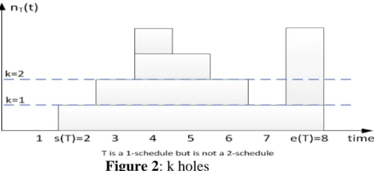
scheduled inside Ω is such that F(i) ⊆Ω. A time-unit t is then a k-hole for T, where k is some positive number, if there exists time-units t, t’, t” such that:
- t’ < t < t”;
- Inf(nT(t’), nT(t”)) > nT(t) = k (in the following figure 2,
time–unit 6 is a 2-hole and time-unit 7 is a 1-hole). Clearly, T is a feasible schedule if only if, for any k in {0..m-1}, it has no k-hole. This leads us to introduce the intermediate notion of schedule: the pre-schedule T is a k-schedule if T has no l-hole for l = 0..k-1, or, equivalently, if the function t -> Inf(k, nT(t)) has a pyramidal shape. The time
diagram of Figure 2 represents a pre-schedule which is a 1-schedule, but not a 2-schedule since time-unit 7 is a 1-hole. Clearly, a feasible schedule is a m-schedule and conversely.
Figure 2: k holes
The family of time-windows F(i), i = 1..n, is stable with respect to the precedence relation << if, for any pair of jobs Ji, Jj such that Ji << Jj, we have: ri 2 rj and di 2 dj. The
following result states that we may assume, without any loss of generality, that our input family of time windows is stable with respect to the precedence relation <<:
Proposition 1: Let I = (J, F, <<, m) be an instance of the
NON-IDLE0 problem. There exists an instance I’ = (J, F’,
<<, m), which may be obtained from I through constraint propagation, which admits the same set of feasible solution as f, which is such that: F’ is stable with respect to << and, for any I, F’(i) ⊆ F(i).
Since the goal of this paper is mainly to provide a characterization of the feasible instances of the NON-IDLE0
problem, together with recognition and makespan minimization algorithms, we proceed in several steps. First, we use the Konig-Hall Theorem related to matchings in bipartite graphs in order to characterize the instances which admits a m-matching. Then, we show that any m-matching may be turned into a pre-schedule. We keep on by identifying a structural property which is going to make possible turning this pre-schedule into a feasible schedule. Finally, we translate this mathematical characterization into a recognition algorithm.
3.2. Existence of a m-matching and of a pre-schedule. Let I = (J, F, <<, m) some NON-IDLE0 instance. For any
interval Ω, we denote by J(Ω) the set of all jobs Ji, such that
F(i) ⊆ Ω. Then one may derive in a straightforward way from classical Konig-Hall Theorem related to the existence of generalized matching in bipartite graphs that:
Proposition 2: The instance (J, F, <<, m) admits a
m-matching if and only if, for any interval Ω of N, we have Card(J(Ω)) 1 m.Card(Ω).
The next property mainly derive from the stability of F. It will help us in dealing with the precedence relation <<.
Proposition 3: The instance (J, F, <<, m) admits a
pre-schedule if an only if it admits a m-matching.
Principle of the proof: starting from a m-matching T, one
only has to iteratively exchange T(i), T(j) values in order to make T compatible with the << precedence relation.
3.3. Existence of A Feasible Schedule.
Let I = (J, F, <<, m) our NON-IDLE0 instance. If the
condition provided by Proposition 3 is satisfied, we easily become able to produce some pre-schedule T. However, such a pre-schedule may have k-holes and thus may not fit the “pyramidal” property required for the feasible schedules. This section will provide an additional necessary and sufficient condition so that an instance I = (J, F, <<, m) admits some feasible schedule. Before deriving this condition, we first give two simple lower bound properties which must be met by such a feasible schedule and then introduce the notion of propagation path which will prove to be a quite useful tool either to transform a pre-schedule into a feasible schedule or to prove the no existence of such a feasible schedule.
Let Ω be an interval of N. We denote by Int(Ω) the set of intervals which are contained into Ω and by λ(Ω) the integer value Sup ω∈ Int(Ω) 1Card(J(ω))/Card(ω)2. Then the meaning
of those definitions comes in an immediate way through the almost trivial following lemma:
Lemma 1: Let T some be m-matching of I = (J, F, <<, m)
and let Ω be an interval of N. There must exist at least one time-unit in Ω such that at least λ(Ω) machines are busy. We understand the main role of λ(Ω) is to provide us with a lower bound of the number of machines which are going to be necessary if we want to succeed in scheduling the jobs of J(Ω). Notice that if Ω is a T-block, then we have λ(Ω) 4 1Σt ∈Ω nT(t)/Card(Ω)2, since, in this case, J(Ω) is exactly the set
of the jobs which are scheduled inside Ω.
Let us assume now that Ω1 and Ω2 are two intervals of N
such that Ω1 Dom Ω2. If we denote by µ(Ω1, Ω2) the value
Lemma 2: In any feasible schedule of I = (J, F, <<, m), at
least µ(Ω1, Ω2) jobs are scheduled in the interval Mid(Ω1,
Ω2) .
Also, the following two properties, which come in a straightforward way and which are related to T-blocks, will be useful in order to derive the main characterization result:
Lemma 3: Let T be some m-matching of I = (J, F, <<, m)
and let Ω1 and Ω2 be two connected T-blocks. Then Ω1∪Ω2
is a T-block and λ(Ω1∪Ω2) 2 Sup(λ(Ω1),λ(Ω2)).
Lemma 4: Let T be some m-matching of I = (J, F, <<, m), let
Ω1 be a T-block, and let Ω1 be an interval such that Ω1∩Ω2
is empty. If, for any pair (u, t) in Ω1 * Ω2, nT(u) 2 nT(t)
(respectively nT(u) > nT(t)), then λ(Ω1) 2 λ(Ω2)) (respectively
λ(Ω1) > λ(Ω1)).
Given a m-matching T, we now define what is a propagation path of T. We first define the propagation graph G = (H, E(T)) as the labeled directed graph whose node set is the interval H = {rmin, .., dmax} of the possible values for T, and
the arc set E(T) is defined by:
- [t, t’] ∈ E(T)) iff t 3 t’ and there is at least one job Ji
which is scheduled at t and which is such that t’ ∈ F(i). - If job Ji is scheduled at t and t’ ∈ F(i), then Ji is said to be
a label of the arc [t, t’].
Then, a propagation path of T is an elementary path γ = (t0, ..,
tk) of G(T). The sub-path of γ from ti to tj will be denoted by
γ(ti , tj ). The length L(γ) of γ is the value k + 1 (that means
the number of vertices of γ), and the extended length L*(γ) of
γ is the sum Σs = 1..k |ts – ts-1|.
This propagation path γ is monotone if the sequence (t0, .., tk)
is either decreasing or increasing. It is no-cross if for any r
∈{1..k}, we have either tr > Sup i = 1..r-1 ti or tr > Inf i = 1..r-1 ti, .
Clearly, the no-cross property may be viewed as a weak version of monotonicity. It is labeled when all its arcs are assigned with labels, that means when, with any arc in γ, we decided to associate some job Ji whose value T(i) is likely to
be modified through shiftpropagation along γ.
The path γ is said to be fitted if it is labeled and satisfies Card(T-1(tk)) < m. Of course, we understand that if f γ = (t0, ..,
tk) is a propagation path of G(T), which is fitted and provided
with the labeling σ = (Ji(0), .., Ji(k-1)), then we brcome able to
modify the m-matching T and get another m-matching T’ = Trans(T, γ, σ) by setting T’(Ji(p)) = tp+1 for any p = 0,.., k-1.
Let T be a pre-schedule and let γ = (t0, .., tk) be a propagation
path of the graph G(T). If γ has at least one labeling σ such that T’ = Trans(T, γ, σ) is a pre-schedule, then γ is said to be compatible with the precedence relation << (<<-compatible in short). Then two following lemmas show the way no-cross propagation paths may turn a pre-schedule into another one:
Lemma 5: Let T be a pre-schedule and let us assume that γ = (t0, .., tk) is a propagation path of G(T) from t0 = u to tk = v.
Then there exists a no-cross propagation path from u to v in G(T).
Proof: Assume that γ is not no-cross and let tr (2 2 r 2 q) be
the first node of γ such that min i = 1..r-1 ti < tr < max i = 1..r-1 ti.
From the definition of tr, we know that there is a smallest
index s (0 2 s 2 r - 2) such that tr belongs to I(ts, ts+1). Thus
[ts, tr] is an arc of G(T) and the concatenation γ(t0, ts). [ts, tr] is
no-cross. The above transformation may then be iterated while the current propagation path is not no-cross.
Lemma 6: Let T be a pre-schedule and let us assume that γ = (t0, .., tk) is a propagation path of G(T) from t0 = u to tk = v,
where Card(T-1(tk)) < m. Then there exists a no-cross and
<<-compatible propagation path from u to v in G(T).
Sketch of the proof. Define the extended length of such a
path γ in G(T) as the sum Σi = 1..kti – ti-1, and consider a
propagation path γ from u to v with minimal extended length and whose length is maximal among the paths with minimal extended length. Assume also that γ is not <<-compatible and let σ = (Ji(0), .., Ji(k-1)) be a labeling of γ. The jobs of the
labeling are called the moving jobs, while the other jobs are called the static jobs. Since T is a pre-schedule and γ is not <<-compatible, << is violated in T’ = Trans(T, γ, σ) because an inversion either between a static job J’ scheduled at t’ and a moving job Ji(s) scheduled at ts+1 or between two moving
jobs Ji(s) and Ji(r) respectively scheduled at time ts+1 and tr+1. In
both case, one checks that it is possible to rearrange path γ in order to get a contradiction on the minimality of γ.
Let T be a pre-schedule and let u be a time-unit such that nT(u) > 0. The next lemma provides us with an important
property of the set AT(u) of the time-units that may be
reached from u by the propagation paths of G(T).
Lemma 7: The set AT(u) is a T-block.
We are now able to describe and state the structural condition which must be met by a NON-IDLE0 instance I =
(J, F, <<, m) so that it admits some feasible schedule.
Theorem 2: The instance I = (J, F, <<, m) of NON-IDLE0 is feasible if and only if:
1. For any interval Ω of N, Card(J(Ω)) 1 m.Card(Ω). 2. For any sequence (Ω1,..Ωp) of intervals of N, such
that Ω1 Dom…Dom Ωp ,we have:
Card(J - ∪ s = 1..p J(Ωs) ) 2 Σs = 1..p-1µ(Ωs, Ωs+1).
Sketch of the Proof.
The “only if” part of the proof is a straightforward consequence of propositions 2 and 4 and lemmas 1, 2, 3
Before dealing with the “if”part, let us recall that, for any k = 1..m, a pre-schedule T is a k-schedule if T has no l-hole for any l = 0..k-1. So we adapt the definition of the quantity
µ(Ω1,Ω2), where Ω1 and Ω2 are two time intervals such that
Ω1 Dom Ω2, to k-schedules by setting: µ∗(Ω1,Ω2, k) =
Lemma 8: Let Ω1 and Ω2 be two time intervals such that Ω1
DomΩ. In any k-schedule of I = (J, F, <<, m), at least
µ∗(Ω1,Ω2, k) jobs are scheduled in the interval Mid(Ω1, Ω2).
In order to prove the “if” part, we extend the statement of Theorem 2 to k-schedules and prove it by induction on k. Using k-schedules allow us to try to perform an inductive reasoning in order to prove Theorem 2, and to prove the following inductive extension of Theorem 2 to k-schedules :
Inductive Formulation of Theorem 2: The instance I = (J,
F, <<, m) of NON-IDLE0 admits at least one k-schedule if
and only if the following two conditions are satisfied: 1. For any interval Ω of N, Card(J(Ω)) 1 m.Card(Ω). 2. For any sequence (Ω1,..Ωp) of intervals of N, such
that Ω1 Dom… Dom Ωp ,we have: Card(J -
∪
s = 1..pJ(Ωs) ) 2 Σs = 1..p-1µ∗(Ωs, Ωs+1,k).
In order get it, we proceed by induction on k. More precisely, we show that if an instance I = (J, F, <<, m) of the NON-IDLE0 problem has at least a k-schedule and no
(k+1)-schedule, then there exists a sequence of intervals that does not satisfy condition 2 of the above statement. In order to get such a sequence, we consider a k-schedule T of I, such that: - T has a minimum number of k-holes;
- the vector (NT(m),.., NT(1)), where NT(j) = Card( t such
that nT(t) = j}), is lexicographically minimum.
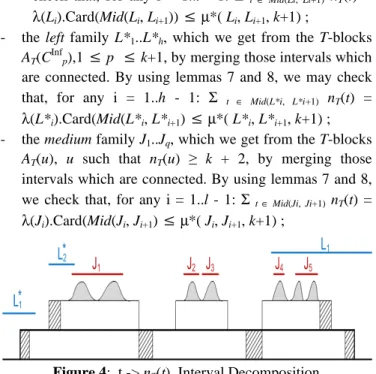
The graph of the piecewise constant function t -> nT(t) may
be decomposed into 3 parts:
- a left part, which is an increasing piecewise constant function: we denote by CInfp, 1 1 p 1 k+1, the smallest
time-unit at which the stair height is at least equal to p; - a right part, which is a decreasing piecewise constant
function: we denote by CSupp, 1 1 p 1 k+1, the largest
time-unit at which the stair height is at least equal to p; - a medium part, made of the time-units u such that nT(u) 4
k + 1, and such that at least one time-unit is a k-hole.
1
12345678211t -> 123341 567869ABACD9
From the minimality of T, we easily get that the propagation graph G(T) is such that there is no propagation path:
- from t which satisfies nT(t) 4 k + 2 to a k-hole; (E1)
- from CSupp or CInfp to a k-hole; (E2)
- from time-units CSupp to CSupj + 1, 1 1 j < p; (E3)
- from time-units CInfp to CInfj + 1, 1 1 j < p; (E4)
From what precedes, we deduce 3 families of intervals: - the right family L1..Ll, which we get from the T-blocks
AT(CSupp), 1 1 p 1 k+1, by merging those intervals
which are connected. By using lemmas 7 and 8, we may
check that, for any i = 1..l - 1: Σ t ∈ Mid(Li, Li+1) nT(t) =
λ(Li).Card(Mid(Li, Li+1)) 1 µ*( Li, Li+1, k+1) ;
- the left family L*1..L*h, which we get from the T-blocks
AT(CInfp),1 1 p 1 k+1, by merging those intervals which
are connected. By using lemmas 7 and 8, we may check that, for any i = 1..h - 1: Σ t ∈ Mid(L*i, L*i+1) nT(t) =
λ(L*i).Card(Mid(L*i, L*i+1) 1 µ*( L*i, L*i+1, k+1) ;
- the medium family J1..Jq, which we get from the T-blocks
AT(u), u such that nT(u) 4 k + 2, by merging those
intervals which are connected. By using lemmas 7 and 8, we check that, for any i = 1..l - 1: Σt ∈ Mid(Ji, Ji+1) nT(t) =
λ(Ji).Card(Mid(Ji, Ji+1) 1 µ*( Ji, Ji+1, k+1) ;
Figure 4: t -> nT(t) Interval Decomposition
Because of (E1, .., E4), those intervals define distinct connected blocks, with non empty space between them. Still, since we may have L*1 ∩ J1 2 Nil or Ll ∩ Jq 2 Nil,
we merge once again the connected intervals of those three families. Then we get a sequence of non connected intervals M1..Mr, of disjoint T-blocks such that M1 Dom .. Dom Mr and
number of jobs which is in ∪j = 1..r J(Mj) is not large enough
to avoid the existence of a k-hole. Then we conclude.
IV. POLYNOMIAL ALGORITHMS
4.1. A Exact Polynomial Algorithm for the NON-IDLE0
Problem
The proof of Theorem 2 is not an algorithmic proof, since it involves an hypothesis about doubly minimality which has no algorithmic interpretation. In this section, we first show that a forbidden pattern of intervals may also be found from any k-schedule which satisfies a weaker set of conditions than that of the doubly minimal k-schedule T considered in the proof of Theorem 2. It allows us to get conditions which might be used as halting test inside the “while” loop of a recognition algorithm, and to derive a exact polynomial algorithm which solves NON-IDLE0, and whose correctness
mainly relies on this new set of sufficient conditions.
So, let T be a k-schedule and let U and V be two disjoint sets of time-units: PP(U, V) is the set of propagation paths of G(T) which start in U and end into V, Hole(k) is the set of units t which are k-holes, and Top(k) is the set of time-units t which satisfies nT(u) 4 k + 2. Then we may state:
Theorem 3. Let I = (J, F, <<, m) be an instance of
NON-IDLE0, and k in {1, .., m-1}. Let us assume that T is a
k-schedule of I such that the following conditions are satisfied: 1. T is not a (k+1)-schedule; 2. PP(Top(k) ∪ {CInf1,..,C Inf k+1} ∪ {C Sup 1,..,C Sup k+1}), Hole(k)) is empty; 3. PP(Top(k), {CInf1 -1,..,C Inf k+1 -1} ∪ {C Sup 1 +1,.., C Sup k+1 +1}) is empty;
4. For j = 2..k+1, PP({CSupj}, { CSupj-1 + 1}) is empty;
5. For j = 2..k+1, PP({CInfj}, { CInfj-1 - 1}) is empty;
Then the instance I has no (k+1)-schedule.
This result gives rise to the following algorithm SEARCH-SCHEDULE(J, F, <<, m) which provides, for any I = (J, F, <<, m), either a feasible schedule of I or a k-schedule T which satisfies 1..5 above: Hole(k), Top(k), CSupp , CInfp
denote here variables related with the current k-schedule T.
Algorithm SEARCH-SCHEDULE(J, F, <<, m):
T <- Matching(J, F, m); (*Computation of an initial m-matching, through a standard matching procedure*) If T does not exist (*Condition of Propositions 2 and 3*) then SEARCH-SCHEDULE <- Fail Else
T <- Pre-Schedule(J, F, m, <<, T); (*Turn T into a pre-schedule through proposition 3*)
k <- Sup l = 0..m l such that T is a l-schedule; Not Stop;
While k < m and Not Stop do Search, according to this order, for a propagation path γ in:
oPP(Top(k) ∪ {CInf1,..,CInfk+1} ∪ {CSup1,..,CSupk+1},
Hole(k));
oPP(Top(k), {CSup1 +1,.., CSupk+1 +1} ∪ {CInf1 -1,..,
CInfk+1 -1});
o∪j = 2..k+1 PP({CSupj, CInfj }, {CInfj-1 -1 , CSupj-1 +1});
If Failure(Search) (*γ does exist*) then Stop Else Let σ be a label of γ; T <- Trans(T, γ, σ); If k = m then SEARCH-SCHEDULE <- T else SEARCH-SCHEDULE <- Fail;
Theorem 4. SEARCH-SCHEDULE solves, in an exact way, the NON-IDLE0 problem in polynomial time.
Sketch of the proof: as for correctness, it derives from the
proof of Theorem 2. As for complexity, one checks that, once an initial m-matching has been computed, time-windows may be restricted in such a way that the size of their union be polynomial bounded by the number n of jobs, and that the number of time the path search instruction for a given k, may be polynomialy bounded in n and k. This provides us with the key argument for the time-polynomiality of our algorithm.
4.2. An Exact Polynomial Algorithm for the NON-IDLE1
Problem
Makespan minimization is contained into feasibility testing, and comes in a simple way through the following process:
Makespan-Min-No-Idle-Schedule Algorithm.
Input: the instance I = (J, F, <<, m)
Output: a no idle feasible schedule or a Failure1signal; Initialize T through SEARCH-SCHEDULE;
If Failure(Initialize) then Failure Else 1 Not Stop;
While Not Stop do
∆ <- Makespan(T);
Let t1 and t2 respectively the smallest and largest
active time-units according to T;
For any job Ji∈ J, set F∆(i) = F(i 5 { t1 + 1, t2};
T-Aux <- SEARCH-SCHEDULE(J, F∆, <<, m); If T-Aux 3 Failure then T <- T-Aux Else
For any job Ji∈J, set F∆(i) = F(i) 5{ t1,.., t2-1};
T-Aux <- SEARCH-SCHEDULE(J, F∆, <<, m); If T-Aux 3 Failure then T <- T-Aux Else Stop. Makespan-Min-No-Idle-Schedule <- T ;
Theorem 5: The above Makespan-Min-No-Idle-Schedule
algorithm solves, in an exact way, the Makespan Minimization NON-IDLE1 Problem in Polynomial Time.
Sketch of the Proof: the basic point here is that if T is some
feasible schedule with active time-unit set ACT(T) = [a, b] , and if there exists a feasible schedule T’ with smaller makespan than T, then T’ may be computed inside the time-window [a, b].
V. CONCLUSION
We just studied a variant of the m-machine non-idling problem: a structural feasibility criterion as well as polynomial algorithms have been provided. However, several questions about the complexity of more general problems with the same HNI constraints are still open: it would be interesting to get the complexity status of the variant of the problem which corresponds to the case when the non-idling constraint has only to be satisfied on each machine.
REFERENCES
Baptiste.P. (2005): “Scheduling unit tasks to minimize the number of idle periods”; Research Report, CNRS LIX Lab..
Chretienne.P (2008): “Single-machine scheduling without intermediate delays”; Disc. App. Maths 13-156, p 2543-2550.
Jouglet.A (2012): “Single-machine scheduling with no-idle time and release dates to minimize a regular criterion”, Journal of Scheduling 15 (2), p 217-238.
Valente .J.M. Alves.R (2005): “An exact approach to early/tardy scheduling ”, Computers/OR 32, p 2905-2917.
Landis.K (1983): “Group technology and cellular manufacturing in Westvaco”, Project Report in IOM 581, School of Business, University of Southern California.
Irani.S, Pruhs.K (2005): “Algorithmic problems in power management”, ACM Press, vol 36, p 63-76, New York, USA.