an author's
https://oatao.univ-toulouse.fr/25376
https://doi.org/10.1016/j.compstruct.2020.111949
Montagne, Benoît and Lachaud, Frédéric and Paroissien, Eric and Martini, Dominique and Congourdeau, Fabrice
Failure analysis of single lap composite laminate bolted joints: comparison of experimental and numerical tests.
(2020) Composite Structures, 238. 1-13. ISSN 0263-8223
Failure analysis of single lap composite laminate bolted joints: Comparison
of experimental and numerical tests
Benoit Montagne
a, Frédéric Lachaud
a,⁎, Eric Paroissien
a, Dominique Martini
b,
Fabrice Congourdeau
baInstitut Clément Ader (ICA), Université de Toulouse, ISAE-SUPAERO, INSA, IMT MINES ALBI, UPS, CNRS, 3 Rue Caroline Aigle, 31400 Toulouse, France bDassault Aviation, 78 Quai Marcel Dassault, 92210 Saint-Cloud, France
Keywords: Composite materials Bolted joints Finite element analysis Damage model
A B S T R A C T
Carbonfiber reinforced plastics (CFRP) are widely used in aircraft industry because of their high mechanical properties. However these properties considerably drop when composite materials are drilled and bolted. Thus, it is important to master the composite bolted joint behavior to avoid a structural failure. Experimental test on single lap bolted joints with various end distance have been led. The failed specimens are analysed thanks to XR computed tomography (XR-CT) and digital image correlation (DIC). The results are compared with a three dimensionalfinite element model involving a progressive damage model for the composite material. It is based on a progressive damage model of the composite material. The global behavior and the damages computed are in good agreement with the experimental results. But, contrary to the experimental observations, the computed damage scenarios are the same for all the tested end distance.
1. Introduction
Carbonfiber reinforced plastics (CFRP) are more and more used by aircraft manufacturers because they are considered as a mean to in-crease future aircraft performances. In spite of their interesting me-chanical properties, composite materials are considerably weakened when they are drilled and bolted. Moreover aircrafts count thousands of fasteners. Thus manufacturers need to master the behavior of bolted joints in order to optimize them. Currently, bolted joints are mainly designed (lay-up and dimensions) thanks to experimentally based guidelines like those established by Hart-Smith[1]. These guidelines aim at ensuring bearing failure mode of the bolted joint because it is a progressive failure mode. The end distance (e) is generally higher or equal to 2.5 times the bolt diameter (d) to avoid shear-out and cleavage failure. The width (w) is generally equal to 5d to avoid net section failure. The laminate should contain between 1/8 (12.5%) and 3/8 (37.5%) of plies in each one of the four orientations (i.e. 0°, 45°,−45° and 90°).
Bolted CFRP joints behaviors are still difficult to simulate up to failure. Different methods have been proposed in literature[2–5]. One of the most common failure analysis method used in industry is the characteristic length method [6–9]. Stresses are analyzed at a char-acteristic distance of the center of the hole. However this length has to
be determined experimentally so it is expensive. Kweon et al. [10] propose a method to determine this length thanks to the use of afinite element model (FEM). In the same way Zhang et al.[11]develop a numerical method to determine this length using progressive damage method (PDM). Authors developed PDM for failure predictions of me-chanical joints. First it starts with open hole plates[12,13]. Then it is adapted for bolted joints [11,14–17] to predict joint strength and failure modes. Nevertheless these phenomena are not easy to observe during tests because they are often hidden by the fastener. That is why simulations on three-dimensional (3D) FEM using PDM have been performed to quantify the damage of the material.
An important experimental database on composite bolted joints owned by DASSAULT AVIATION has been analyzed. The main result of this analysis (discussed in[18]) is that the end distance is the most important design parameter of the joint. The failure modes observed vary from cleavage/shearout (brittle failure mode when e is small) to bearing failure (progressive failure mode when e is large enough). w, stacking sequence and load orientation has also been studied but they have a lower influence on the composite bolted joint behavior. These results agree with the ones obtained by Collings [19]. New tests to simplify boundary conditions and improving in and post situ observa-tions (thanks to DIC and XR-CT) are lead on specimens with various end distance.
https://doi.org/10.1016/j.compstruct.2020.111949
⁎Corresponding author.
First, the specimens preparation is detailed and the results are analyzed in this paper. Then the relatedfinite element model using a UMAT to simulate the nonlinear behavior of the composite material is described. The results extracted from the simulations are then com-pared with the experimental one. In particular the damage variables are compared with the XR-CT to confirm the simulated damaging scenarios.
2. Experimental test 2.1. Test specimen
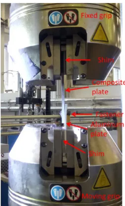
In order to analyze to what extent, e has a preponderant role on the failure modes, single lap joint specimens with various e have been tested. These specimens consist in CFRP/aluminum joints as illustrated in Fig. 1. The CFRP part is a laminate made of unidirectional (UD) prepreg T700/M21 manufactured by Hexcel. This plate contains 50% of plies oriented at 0°, 40% of ± 45° and 10% of 90°. This laminate is close to the classical design rules[1]and it might have similar cleavage/ shearout and bearing failure modes depending on the end distance. Moreover it is currently used on aircraft. The dimensions are detailed in theTable 1.
The second plate of the joint is made of aluminum 2024 alloy. Its length is 100 mm, its width 80 mm and its thickness 4 mm. The hole is drilled in the aluminum at e = 20 mm. CFRP and aluminum plates are jointed with a 7.92 mm countersunk fastener in steel (NAS1155 stan-dard). A 20 N.m torque is applied in two steps to tighten the plates and limit the relaxation of the fastener.
2.2. Test facilities and procedure
The composite plate is hold in the upper grip of an INSTRON 8800 250 kN hydraulic tensile machine, the aluminum plate is hold in the lower jaw. Shims are used to ensure the alignment of the plates and limit the bending of the joint. A (DIC) device is used to follow the displacement of the countersunk head and the upper face of the com-posite plate. This system is made of two cameras with 16 mm lenses and a computer using VIC Snap (Correlated Solutions) software for the ac-quisition and VIC 3D 7 software (Correlated Solutions) for the post treatment. Quasi-static tests are controlled with prescribed displace-ment at a speed of 0.5 mm/min with unload cycles. The load is applied until the failure of the joint. The set-up of the test is presented on the scheme Fig. 1 and the dimensions of the specimens are detailed in Fig. 2.
2.3. Results
2.3.1. Load-displacement behavior
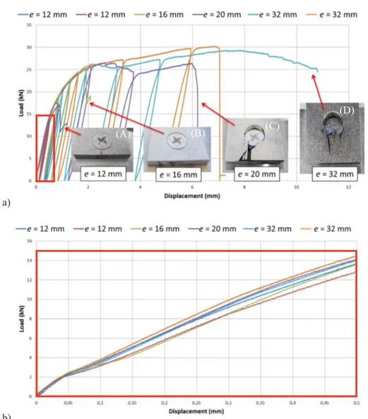
Global load displacement behavior and a zoom on the linear part are presented inFig. 3. The displacements and forces presented in this figure are provided by the tensile machine.
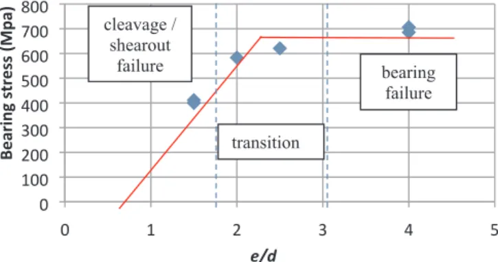
All the curves are very close in the linear part i.e. the stiffness of the joint does not depend on e. Afirst stiffness variation is observed around 0.04 mm. It is due to the contact behavior of the surfaces that varies from sticking to slipping. This phenomenon is also observed during the unloading–reloading cycles. This stiffness variation leads to loops in the load–displacement curves[20]. Specimens with e = 12 mm are thefirst to fail at a load of approximately 17 kN. Their failures are characterized by delaminations, matrix andfibers breakage behind the bolt and also on the edge of the composite plate as shown on picture (A) inFig. 3. Those phenomena also occur during the test on the specimen with e = 16 mm but the failure is reached for a higher load. Contrary to the e = 12 mm specimen the outer ply of the e = 16 mm specimen has not failed (picture (B) inFig. 3). The e = 20 mm specimen fails for ap-proximately the same load as the e = 16 mm specimen but for a much higher displacement. Important delaminations are observed behind the bolt on the composite plate. Finally when e is sufficiently large (e = 32 mm), delamination of the outer ply are concentrated just be-hind the bolt and do not propagate until the end edge. The maximal load and displacement are higher than the ones obtained for the other specimens. The orange curve (e = 32 mm) differs from the light blue one (e = 32 mm): the important load drop observed on the orange curve is due to thefirst thread bolt failure. This phenomenon is not observed on the other curve because the specimen failed in bearing mode. The bearing stress (i.e. the maximum load divided by the dia-meter and the thickness) is represented as function of the e in theFig. 4. These results are in agreement with the literature [19]in terms of failure modes and bearing stresses: the bearing stress at failure is nearly proportional to e when e is small and constant when e is large enough as illustrated inFig. 4. The failure mode is cleavage/shearout when e is sufficiently small and bearing otherwise.
2.3.2. Post-failure analysis
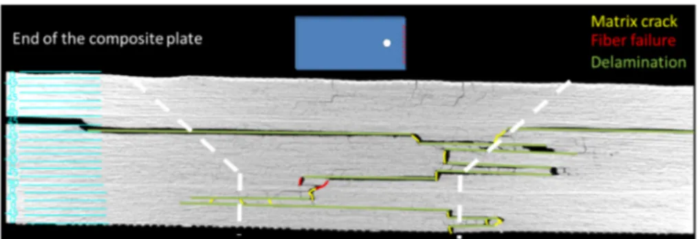
The failed specimens were analyzed thanks to XR tomography. Only the e = 12 mm and e = 16 mm specimens are studied here because it was not possible to dismantle the fastener of the e = 20 mm and e = 32 mm specimens without breaking the composite plate. TheFig. 5 is a slice of the end edge of the composite plate e = 12 mm extracted from the tomography.Fig. 6is a slice at the mid plane of the e = 12 mm specimen. Only some of the visible degradations have been highlighted. These degradations are categorized from visual inspection according to their location and their shape. A horizontal crack located between two plies is considered as a delamination. A vertical or diagonal crack is considered as afiber or matrix failure according to the ply considered and to the observations of other slices.
Fig. 1. Set-up of the test on single lap bolted joint specimen.
Table 1
Dimensions of the composite specimen (in mm).
e Total length (l) w Thickness (t)
32 162 40 5.4
20 152 40 5.4
16 146 40 5.4
Fig. 2. Dimensions of the composite (blue) and aluminum (grey) plates.
a)
b)
(A)
(B)
(C)
(D)
Delaminations and matrix cracks are mainly observed. Delaminations seem to start at the end of the plate and then progress in the laminate until reaching the hole. No degradation has been observed in the vicinity of the hole in the view cutFig. 6due to artefacts on the tomography. The XR tomography of the e = 16 mm specimen does not present those artefacts thus some degradations could be observed in the vicinity of the hole. They are presented inFigs. 7 and 8.
According to these XR-CTs the lower plies of the laminate are more damaged than the upper plies. A hypothetical scenario might be ela-borated basing on these results. The degradation seems to start in the cylindrical part of the hole and then propagates in the lower plies of the laminate because these plies are more damaged than the upper ones. The matrix of the plies oriented at 0° in the cylindrical part might fail. Cracks are growing until reaching the interface with another ply. Then delamination occurs and the degradation keeps getting up in the la-minate. Of course this is a hypothetical scenario and it will be validate with a more complete test campaign in future work.
3. Numerical test 3.1. Model geometry
Single lap joint specimens are modelled using Abaqus CAE. The plates and the fastener are designed with the same width and end distances as the specimens (detailed in Table 1). The lengths of both plates are shortened of 50 mm corresponding to the lengths hold in the jaws of the tensile machine. The bolt and nut are modelled by a single part.
3.2. Material modelling
The bolt and nut in steel has an elastic behavior with a Young’s modulus of 210 GPa and Poisson’s ratio of 0.3. The other materials have
nonlinear behavior as detailed below.
3.2.1. Nonlinear behavior of the composite material
The nonlinear behavior of the composite material is implemented within a homemade user script referring to UMAT in the Abaqus en-vironment. It is based on the work of Matzenmiller, Lubliner and Taylor (MLT)[21]and modified in[22]. This law works at the ply scale. De-gradation of the material is described with failure criteria corre-sponding to different solicitation modes. The Young moduli (Ejk) (1 for
thefibers direction, 2 for the transverse direction, 3 for the out of plane direction) of the composite material are reduced in the compliance matrix (Cdam) in Eq. (1) using damage variables (Di) with
0 < Di < Di,max. Each damage variable is limited to a (Di,max) for two
reasons. Thefirst one is to avoid numerical issues when Diis close to 1.
And the second one is to keep a compressive stiffness in elements when they are totally failed. This value corresponds to the ratio of transverse over longitudinal moduli for the fiber direction. It is set to 0.99 otherwise. = ⎛ ⎝ ⎜ ⎜ ⎜ ⎜ ⎜ ⎜ ⎜ ⎜ ⎜ − − − − − − ⎞ ⎠ ⎟ ⎟ ⎟ ⎟ ⎟ ⎟ ⎟ ⎟ ⎟ − − − − C 0 0 0 0 0 0 0 0 0 0 0 0 0 0 0 0 0 0 0 0 0 0 0 0 ν ν ν ν ν ν dam 1 E (1 D ) E E E 1 E (1 D ) E E E 1 E 1 G (1 D )(1 D ) 1 G 1 G 11 1 12 11 13 11 12 11 22 2 23 22 13 11 23 22 33 12 4 4b 23 13 (1) ≈ − D E E 1 max 1, 22 11 (2)
These damage variables are calculated in Eq.(3)based on variables (ϕi) which represent for the degradations associated with a given failure criterion. ⎛ ⎝ ⎜ ⎜ ⎜ ⎞ ⎠ ⎟ ⎟ ⎟ = ⎛ ⎝ ⎜ ⎜ ⎞ ⎠ ⎟ ⎟ ⎛ ⎝ ⎜ ⎜ ⎜ ⎞ ⎠ ⎟ ⎟ ⎟ D D D D ϕ ϕ ϕ ϕ 1 1 0 0 0 0 1 0 0 0 1 0 0 0 0 1 b b 1 2 4 4 1 2 4 4 (3)
These variablesϕiare derived from the failure criteria (fi) with an
evolution law[23]in order to describe the damageable behavior of the material: = ci max( fi, 1) (4) ⎜ ⎟ = − ⎛ ⎝ − ⎞ ⎠ > ϕ exp c m c 1 1 ( 1) i im i i i (5) where miis a related parameter which drives the evolution ofϕi. The
0
100
200
300
400
500
600
700
800
0
1
2
3
4
5
e/d
Bearing stress (Mpa)
bearing
failure
transition
cleavage /
shearout
failure
Fig. 4. Bearing stress as function of e.
higher this parameter is the more brittle the behavior is.
Criteria are computed with the elastic prediction stresses within the plies. The failure modes considered here are: thefiber tensile failure Eq. (6), thefiber compressive failure Eq.(7) (based on Hashin criterion [24]) and the matrix failure Eqs.(8) and (9):
⎜ ⎟ = ⎛ ⎝ < > ⎞ ⎠ + + f σ σ σ σ RT RS 1 11 11 2 122 12 (6) ⎜ ⎟ = ⎛ ⎝ < − > ⎞ ⎠ + f σ σRC 2 11 11 2 (7) ⎜ ⎟ ⎜ ⎟ ⎜ ⎟ = ⎛ ⎝ < > ⎞ ⎠ + ⎛ ⎝ < − > ⎞ ⎠ + ⎛ ⎝ ⎞ ⎠ + + f σ σ σ σ σ σ RT RC R 4 22 22 2 22 22 2 12 12 2 (8) ⎜ ⎟ = ⎛ ⎝ − ⎞ ⎠ − f σ D k σ (1 ) b t R 4 12 4 1 12 2 (9) where: < . > + are the Macaulay brackets, R in the exponent indicate an experimentally identified failure stress: T for the tensile stress, C for the compressive one and S for the shear, Djt-1is the damage variable at
the previous converged loading step of the computation, k is a coe ffi-cient that drives the softening behavior.
The damage variableϕb
4 permits to take into account for the shear nonlinear behavior of the composite material. The related criterion is presented in Eq.(9)and illustrated inFig. 9. In thisfigure the coeffi-cient k is taken equal to 2 i.e. the damage begins when the shear stress is equal to the half of the failure shear stress. Then the shear modulus
progressively decreases until the shear stress reaches the failure limit. The second damage variable is then activated and the failure happens. Finally a delayed damage effect[25]is applied to limit the locali-zation of the damage in the model and to suppress the mesh de-pendency. = − − − D τ exp a D D ̇ 1(1 ( ( 0 ))) (10) where: D0is the damage variable without delay damage effect, τ is the
time constant of the delay damage effect and a is a parameter driving the onset of the delay damage effect. The influence of some numerical parameters on the behavior of an elementary model is presented in Appendix A.
Fig. 6. Slice of the mid plane of composite plate with e = 12 mm.
Fig. 7. Slice of the end of composite plate with e = 16 mm.
Fig. 8. Slice of the mid plane of composite plate with e = 16 mm.
0 0.1 0.2 0.3 0.4 0.5 0.6 0.7 0.8 0.9 1 0 0.1 0.2 0.3 0.4 0.5 0.6 0.7 0.8 0.9 1 0 0.005 0.01 0.015 0.02 0.025 0.03 0.035 ʍ12 ʔ4b ʔ4 Strain Normalized stress Damage
The parameters used in the model are detailed in Table 2. The mechanical properties of the T700/M21 UD ply is extracted from[26]. They have been identified experimentally thanks to elementary tests. Thefibers failure stress in compression σRC
11 is quite higher than the one identified in[26]to take into account for the reinforcement due to the tightening as shown in [19,27]. Its value has been identified experi-mentally. k and mibare identified in[28]thanks to a tensile test on a
[ ± 45°]2slaminate. D1, maxis computed thanks to the Eq.(2).τ and D2/ 4,maxare set to obtain a better convergence of the simulation. Finally, mi
are set to 10 in order to ensure a brittle failure of the corresponding mode.
3.2.2. Nonlinear behavior of the aluminum material
The aluminum plate is assumed to have an elastoplastic behavior based on Von Mises yield criterion using a bilinear law (Fig. 10); in the numerical simulations, this behavior is unbounded in terms of strain. The elastic properties are defined by a Young’s modulus of 70 GPa and a Poisson’s ratio of 0.3. The yield stress is equal to 320 MPa. The second slope is equal to 1070 MPa.
3.3. Mesh, boundary conditions and loading
The boundary conditions are detailed inFig. 11. One edge of the aluminum plate (on the left of the scheme) is clamped. The opposite edge of the composite plate (on the right of the scheme) is rigidly linked to a reference point.
The loading is applied in two steps. First the bolt is tightened using the bolt load defined in Abaqus with an installed tension of 6 kN. The second step is the loading in tension of the composite plate. A dis-placement of 4 mm along x direction is imposed on the reference point. Other degrees of freedom are set to 0. Surface to surface contact using Coulomb’s law is set between the different parts with a coefficient of friction of 0.3 for the plate to plate contact and 0.1 for the bolt to plate contacts [29]. The part with the coarsest mesh is used as the master surface in the contact definition.
The composite plate, the bolt and the aluminum plate are meshed using 3D linear hexahedral elements (24 degrees of freedom per ele-ment, 8 integration points per eleele-ment, linear interpolation) under the normal integration scheme. One element per ply is used in the thickness
of the composite plate. The mesh is refined in the vicinity of the hole as detailed inFig. 12to obtain a length of approximately 0.3 mm in the radial direction with the following mesh.
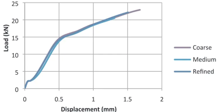
Mesh sensitivity has been tested using three mesh densities: coarse, medium and refined.Fig. 12represents the medium mesh used in this paper. The global behaviour is the same for the three meshes as shown inFig. 13. The model sensitivity to the delay damage effect is detailed in Appendix A.
Table 2
Parameters used to describe the composite behavior in the UMAT.
E11(GPa) E22(GPa) E33(GPa) ν12 ν23 ν13 G12(GPa) G13(GPa) G23(GPa)
117 7.7 7.7 0.34 0.4 0.34 4.8 4.8 2.8
σRT
11 (GPa) σ12RS(GPa) σ11RC(GPa) σ22RT(MPa) σ22RC(MPa) σ12R(MPa) σ23R(MPa) k d1,max d2/4,max τ mi mib
2.2 1.5 1.7 50 300 95 95 2 0.93 0.99 0.01 10 1.75 0 50 100 150 200 250 300 350 400 450 0 2 4 6 8 10 12 Bilinear law Exp. test
True tensile strain (%)
True tensile stress (MPa)
Fig. 10. Assumed elastoplastic behavior under tensile of the aluminum alloy 2024 plate.
Fig. 11. Boundary conditions.
(A) (B) (C)
Fig. 12. Meshes of the different part: (A) composite plate, (B) fastener, (C) aluminum plate. 0 5 10 15 20 25 0 0.5 1 1.5 2 Coarse Medium ZeĮŶed Displacement (mm) Load (kN)
3.4. Results
The applied load is obtained thanks to the reference point linked to the edge of the composite plate for the numerical model. Displacements presented in the followingfigures are equal to the relative displacement between the aluminum and the composite plates as detailed inFig. 14. The displacement on the aluminum plate is measured by doing the mean of the displacement on the red area in order to be consistent with the measure extracted from DIC. No extensometer was used during the test and it is difficult to extract values from a single point on DIC. That is why an average is done on an area. The displacement of the com-posite plate is taken in the symmetry plan at 30 mm of the center of the hole. These simulation results are then directly compared with the re-sults extracted from DIC.
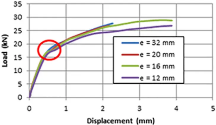
The load/displacement curves for the 4 geometrical configurations are presented inFig. 15.
As observed in the experimental results, initial stiffnesses are almost the same for the different cases. It appears that the shorter the end distance the more important the stiffness loss (circled in red onFig. 15). Convergence troubles are encountered with e = 32 mm and e = 20 mm specimens. It might be due to the damaging pattern that occurs when the end distance is large. The damage of the matrix is presented on Fig. 16for e = 32 mm and e = 12 mm for the comparison. The de-gradation is distributed between the hole and the end edge for e = 12 mm when it is only concentrated behind the bolt for e = 32 mm. This concentration of damage could lead to numerical convergence is-sues. The difference of damage localization between the small and large edge distance is in agreement with the observations made on the failed specimens. The comparison between thefinite element model and the experimental observations are detailed in the next section.
4. Test versus simulation comparisons 4.1. Global behavior
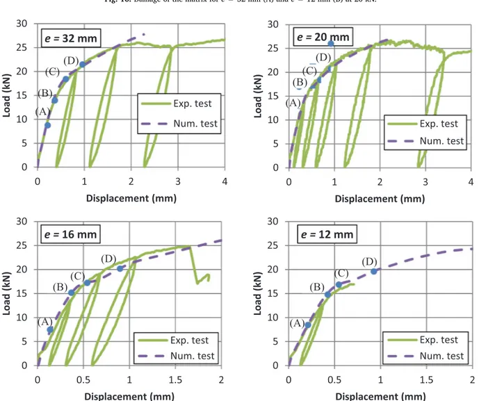
Comparisons between experimental and numerical results are pre-sented in Fig. 17. The simulation resultsfit quite well with the ex-perimental ones until 2 mm relative displacement for the larger end distance cases or until the failure of the specimen for the smaller end distance cases. Thefirst part of these curves (from 0 to 2.5 kN) corre-sponding to the transfer by friction is represented thanks to the step of tightening in the numerical model. Then the load is transmitted through the contact between the plates and the bolt until the end of the test. The linear part of the test (from 0 to approximately 10 kN) is well re-presented by the numerical model but gaps are growing when non-linearities appear. Even if the nonlinear behavior of the joint (load > 10 kN) is well represented for e = 32 mm and e = 20 mm specimens, that is not the case for e = 16 mm and e = 12 mm. For e = 16 mm the load measured in the numerical model is slightly inferior to the ex-perimental one. For e = 12 mm the nonlinearities appear in the model for a higher load than during the test. The points (A), (B), (C) and (D) are referring to the damage scenario detailed in the next section.
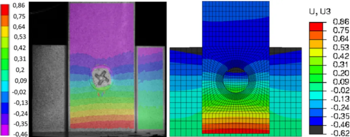
Out of plane displacements obtained by DIC are compared to the ones computed with thefinite element model onFig. 18for e = 32 mm at a displacement of 1 mm. The bending of the aluminum plate is more important in thefinite element model but the results are quite similar. 4.2. Local behavior and failure
According to those results thefinite element model seems to be able to reproduce the behavior of the bolted joint. The behaviors of the joints of thefinite element model for the 4 configurations are quite the same. Thus the stress are very similar and the damage variables too. That is why damage scenario is only made on one of the 4 configura-tions. Moreover no XR-CT has been made on e = 20 mm and e = 32 mm thus the plies’ degradations could not be compared between the experimental and the numerical results. The damages within the composite plate are presented inFig. 19. First, damage of the matrix is observed (A) at a displacement of 0.18 mm in 0° plies oriented but the behavior of the joint is still linear. It starts to be nonlinear when plastic strain appears in the aluminum plate at 0.27 mm. First damage of the fibers (B) due to compression occurs at 0.36 mm in 0° plies and 45° plies until thefirst failure of elements (C) at 0.48 mm in ± 45° plies or-iented at. Thenfirst damage due to tension appears (D) at a displace-ment of 0.86 mm in 0° plies. Finally these damages progress in the material and continually degrade the stiffness of the joint until the end of the computation.
A slice of the XR tomography of thefirst ply (0°) is compared with the computed damage in thefinite element model at the same level of load for the e = 16 mm specimen inFig. 20.Three plies of the three other orientations (−45°, 45° and 90°) are presented inFigs. 21–23and are detailed below.
Failure due to compression (occurring in the area where thefibers are normal to the hole edge) around the hole is not easy to observe with XR-CT because of the diffraction of X-rays on the hole edge. However, the failure offibers in tension (occurring in the area where the fibers are tangent to the hole edge) and compression seems to be well predicted by the FEM. The matrix failure is not as well predicted as thefibers one but the localization of the damaged element is correct. This over-estimation of the damaged area might have various reasons. First the UMAT parameters (i.e. the stresses at failure) could be too small. Second those matrix cracks are two small to appear in the XR-CT. Its resolution is imposed by the length of the observed specimens and could not be too small. Finally the cracks might have closed after dis-mantling the specimen thus it has to be observed during the test thanks to thermal analysis for instance.
The degradations of a−45° ply are detailed inFig. 21. Failure of
Fig. 14. Computation of the displacement between the two plates.
fibers due to compression is observed in the area of contact with the fastener. Fibers broke in tension (highlighted in red) and the ply split (highlighted in yellow) at the left of the hole. A big crack follows the matrix failure of the upper and lower 0° plies.
The 45° ply presented inFig. 22is also surrounded by 0° plies but contrary to the previous −45° one, there is no crack following the matrix failure of the 0° plies. The tensionfiber failure is well predicted. The compressionfibers failure is also predicted but not correctly loca-lized. Once again the damage of the matrix is too important on the FEM. In the 90° ply shown inFig. 23no degradation is observed in the area of contact with the fastener except thefibers failure in tension in the middle. Moreover the big crack that seems to start at the end of the plate and propagating in the material is not reproduced in the FEM. Finally not as much matrix failure as the ones predicted by the FEM are observed in the XR-CT.
Lastly, we observed that the degradations are not homogeneous in the laminate thickness (as shown inFigs. 6 and 8). This phenomenon is also observed in the FEM. Some 0° plies are compared in theFig. 24. The damaged area in the finite element model and in the XR-CT is smaller in the upper plies than in the lower ones.
Thus the FEM gives good results to predict thefibers failure but the matrix damages are over-estimated. It might be due to the absence of out of plane phenomena in the nonlinear behavior of the composite material. The delamination of a ply occurring during the test results in an unloading of this ply because the load is now carrying by the other plies. It is not the case in thefinite element model because no dela-mination is taken into account. Moreover this might be the reason why the load drop observed experimentally does not occur in the numerical model particularly for small e.
Fig. 16. Damage of the matrix for e = 32 mm (A) and e = 12 mm (B) at 20 kN.
5. Conclusions
Experimental tests on single lap bolted joints are lead in order to study the influence of e on their behaviors. Different failure modes are observed according to e. A 3D FEM with nonlinear material behaviors is developed to analyze the degradations occurring within the composite material. The nonlinear behavior of the composite is based on MLT’s formulation. Failure stress criterion modelling matrix and fibers de-gradations are computed to obtain associated damage variables thanks to evolution laws. These variables degrade the Young moduli of the material until its failure. FEM gives good results in comparisons with the XR-CT of e = 12 mm and e = 16 mm specimens. The simulated
damages are the same for all the tested specimens. First, matrix damage appears. Second plastic strain starts in the aluminum plate. Thenfibers are damaging in compressionfirst and after in tension. Finally, all these degradations extend in the material until the end of the computation: when the imposed displacement is reached for e = 12 mm and e = 16 mm specimens or due to numerical issues for e = 20 mm and e = 32 mm specimens. This model is in agreement with the experi-mental results because all numerical curves are nearly superimposed until the failure of the joint. However the load drop occurring at failure and observed in the test results is not reproduced by thefinite element model. Moreover delaminations are observed during the experimental tests. Those out of plane phenomena are not taken into account in the
Fig. 18. Comparison of experimental and numerical out of plane displacements.
Fig. 19. Damage variable in the numerical model.
FEM. It could be possible to observe delamination by adding cohesive zone element between each plies of the laminate with a damageable traction separation law. But it increases a lot the complexity of the model and the computational time. This model will be developed in future work. More tests will be led on single and double lap joints. The evolution of the degradation in the composite material will be observed thanks to XR-CT by interrupting the test at different load level. CRediT authorship contribution statement
Benoit Montagne: Conceptualization, Methodology, Software, Validation, Formal analysis, Investigation, Writing - original draft, Writing - review & editing. Frédéric Lachaud: Conceptualization, Methodology, Software, Supervision. Eric Paroissien:
Conceptualization, Methodology, Supervision. Dominique Martini: Conceptualization, Methodology, Supervision.Fabrice Congourdeau: Conceptualization, Methodology, Supervision.
Declaration of Competing Interest
The authors declare that they have no known competingfinancial interests or personal relationships that could have appeared to influ-ence the work reported in this paper.
Acknowledgement
The authors gratefully acknowledge the French DGAC for finan-cially supporting this study.
Fig. 21. Comparison of the degradation of a−45° ply with the damages in the FEM.
Fig. 22. Comparison of the degradation of a 45° ply with the damages in the FEM.
Appendix A. Identification of the parameters and sensitivity
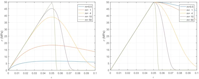
In the definition of the nonlinear behavior law of the composite material the link between the damage variable and the associated failure criteria is made thanks to an evolution law[23]:
= ci max( fi, 1) (12) ⎜ ⎟ = − ⎛ ⎝ − ⎞ ⎠ > ϕ c m c 1 exp 1 ( 1) i im i i i (13) The main interest of this formulation compared to the MLT’s one is that the linear behavior is independent of the parameter mi. TheFig. 25
presents a comparison between the behavior obtained with MLT’s[21]and Xiao’s formulations[23].
With Xiao’s formulation the behavior is the same until the failure stress is reached. Then the softening part depends on mi. The more important mi
is the more brittle the behavior is. Moreover the softening behavior due to miis competing with the delay damage effect. If miis small the delay
damage effect is not used because the variation of the damage variable is smooth. If miis important the delay damage effect is used to reduce the
variation of d and avoid convergence issues. The influence of the parameter τ used in the delay damage effect on an elementary model is analyzed.
Fig. 24. Comparison of the degradation of 0° plies with the damages in the FEM.
0 0.01 0.02 0.03 0.04 0.05 0.06 0.07 0.08 0.09 0.1 0 5 10 15 20 25 30 35 40 45 50 (MPa) m=0.5 m= 1 m= 4 m= 10 m= 50 0 0.01 0.02 0.03 0.04 0.05 0.06 0.07 0.08 0.09 0.1 0 5 10 15 20 25 30 35 40 45 50 (MPa) m=0.5 m= 1 m= 4 m= 10 m= 50
This model is made of on single C3D8 element with the material properties of a UD ply. It is loaded in tension, compression and shear to observe the nonlinear behavior of the composite material. The results for tension and shear for different τ are presented inFig. 26.
If the parameterτ is small enough (less or equal to 1e-2s) the delay damage effect does not modify the element behavior. Delayed damage effect sensitivity has also been studied in the joint model by varying the parameterτ. Its main drawback is to increase the stress at failure of the element. Thusτ has to be set small enough to keep a correct failure stress. But if it is too small the model has convergence issues. TheFig. 27details the influence of the delayed damage effect on the global behaviour of the model. It has convergence issues as soon as damages appear without delayed damage effect. Using a value of τ = 1e-3s permits to have a better convergence but the curve is oscillating. These oscillations correspond to the failure of a row of elements in the composite plate. Increasingτ to 1e-2s permits to avoid oscillations and improve the convergence of the model. This value is used in the following study. Finally the in plane behavior obtained for the elementary model is detailed inFig. 28.
0
500
1 000
1 500
2 000
2 500
0
0.01
0.02
0.03
ɸ
11ʍ
110
20
40
60
80
100
120
0
1,00E-04
5,00E-04
1,00E-03
5,00E-03
1,00E-02
5,00E-02
Shear strain
Shear stres (MPa)
ʏ =
Fig. 26. Sensitivity to the delay damage effect at the element scale for fiber tensile and shearing behaviors.
0 5 10 15 20 25 30 0 0.5 1 1.5 2 2.5 3 Tau=1e-2 Tau=1e-3
tiƚŚouƚ deůaLJed damaŐe eīeĐƚ
Displacement (mm)
Load (kN)
Fig. 27. Sensitivity of the model global behaviour to the delay damage effect.
Longitudinal direction
Transverse direction
In plane shear
References
[1] Hart-Smith LJ. Design and analysis of bolted and riveted joints. Recent advances in structural joints and repairs for composite materials. 2003. p. 211–54.
[2] Agarwal,“Agarwal - [1980] Static strength prediction of bolted joint in composite material.pdf.” 1980.
[3] Hyer MW. Contact stresses in pin loaded orthotropic plates. Int J Solids Struct 1985;21(9):957–75.
[4] Eriksson LI. Contact stresses in bolted joints of composite laminates. Compos Struct 1986;6(1–3):57–75.
[5] Tsai MY, Morton J. Stress and failure analysis of a pin-loaded composite plate: an experimental study. J Compos Mater 1990;24(10):1101–20.
[6] Whitney JM, Nuismer RJ. Stress fracture criteria for laminated composites con-taining stress concentrations. J Compos Mater 1974;8(3):253–65.
[7] Chang F-K, Scott RA, Springer GS. Strength of mechanically fastened composite joints. J Compos Mater 1982;16(6):470–94.
[8] Camanho PP, Lambert M. A design methodology for mechanically fastened joints in laminated composite materials. Compos Sci Technol 2006;66(15):3004–20.https:// doi.org/10.1016/j.compscitech.2006.02.017.
[9] Whitworth HA, Othieno M, Barton O. Failure analysis of composite pin loaded joints. Compos Struct 2003;59(2):261–6.
[10] Kweon J-H, Ahn H-S, Choi J-H. A new method to determine the characteristic lengths of composite joints without testing. Compos Struct 2004;66(1–4):305–15.
https://doi.org/10.1016/j.compstruct.2004.04.053.
[11] Zhang J, Liu F, Zhao L, Chen Y, Fei B. A progressive damage analysis based char-acteristic length method for multi-bolt composite joints. Compos Struct 2014;108:915–23.https://doi.org/10.1016/j.compstruct.2013.10.026. [12] Chang F-K, Chang K-Y. A progressive damage model for laminated composites
containing stress concentrations. J Compos Mater 1987;21(9):834–55. [13] McCarthy CT, O’Higgins RM, Frizzell RM. A cubic spline implementation of
non-linear shear behaviour in three-dimensional progressive damage models for com-posite laminates. Compos Struct 2010;92(1):173–81.https://doi.org/10.1016/j. compstruct.2009.07.025.
[14] Tserpes KI, Labeas G, Papanikos P, Kermanidis T. Strength prediction of bolted joints in graphite/epoxy composite laminates. Compos B Eng 2002;33(7):521–9. [15] Dano M-L, Kamal E, Gendron G. Analysis of bolted joints in composite laminates:
strains and bearing stiffness predictions. Compos Struct 2007;79(4):562–70.
https://doi.org/10.1016/j.compstruct.2006.02.024.
[16] Camanho P, Matthews F. A progressive damage model for mechanically fastened joints in composite laminates. J Compos Mater 1999;33(24):2248–80. [17] Hühne C, Zerbst A-K, Kuhlmann G, Steenbock C, Rolfes R. Progressive damage
analysis of composite bolted joints with liquid shim layers using constant and continuous degradation models. Compos Struct 2010;92(2):189–200.https://doi. org/10.1016/j.compstruct.2009.05.011.
[18] Montagne B, Lachaud F, Paroissien E, Martini D. Failure analysis of composite bolted joints by an experimental and a numerical approach. Presented at the 18th European conference on composite materials (ECCM18), Athens, Greece. 2018. [19] Collings T. The strength of bolted joints in multi directional cfrp laminates.
Composites 1977;8(1):43–55.
[20] Stocchi C, Robinson P, Pinho ST. A detailedfinite element investigation of com-posite bolted joints with countersunk fasteners. Compos A Appl Sci Manuf 2013;52:143–50.https://doi.org/10.1016/j.compositesa.2012.09.013.
[21] Matzenmiller A, Lubliner J, Taylor R. A constitutive model for anisotropic damage infiber-composites. Mech Mater 1995;20:125–52.
[22] Espinosa C, Lachaud F, Michel L, Piquet R. Impact on composite aircraft fuselages. Modeling strategies for predicting the residual strength. Revue des Composites et Matériaux Avancés 2014;24(3):271–318. https://doi.org/10.3166/rcma.24.271-318.
[23] Xiao J, Gama B, Gillespie J. Progressive damage and delamination in plain weave S-2 glass/SC-15 composites under quasi static punch shear loading. Compos Struct 2007;78:182–96.
[24] Hashin Z. Failure criteria for unidirectionalfiber composites. J Appl Mech Jun. 1980;47:329–34.
[25] Allix O, Deü J-F. Delayed damage modelling for fracture prediction of laminated composites under dynamic loading. Eng Trans 1997;45(1):29–46.
[26] Gohorianu G. Interaction entre les défauts d’usinage et la tenue en matage des as-semblages boulonnés en carbone/epoxy PhD Thesis Toulouse, France: Université Toulouse III - Paul Sabatier; 2008
[27] Wang H-S, Hung C-L, Chang F-K. Bearing failure of bolted composite joints. Part 1 experimental characterization. J Compos Mater 1996;30(12):1284–313. [28] Ilyas M. Modélisation de l’endommagement de composites stratifiés carbone époxy
sous impact. Toulouse: Université Toulouse; 2010.
[29] Schön J. Coefficient of friction and wear of a carbon fiber epoxy matrix composi-te.pdf. Wear 2004;257:395–407.