Titre:
Title
: A new efficient RLF-like algorithm for the vertex coloring problem
Auteurs:
Authors
: Mourchid Adegbindin, Alain Hertz et Martine Bellaïche
Date: 2016
Type:
Article de revue / Journal articleRéférence:
Citation
:
Adegbindin, M., Hertz, A. & Bellaïche, M. (2016). A new efficient RLF-like algorithm for the vertex coloring problem. Yugoslav Journal of Operations
Research, 26(4), p. 441-456. doi:10.2298/yjor151102003a
Document en libre accès dans PolyPublie
Open Access document in PolyPublie
URL de PolyPublie:
PolyPublie URL: https://publications.polymtl.ca/3601/
Version: Version officielle de l'éditeur / Published versionRévisé par les pairs / Refereed Conditions d’utilisation:
Terms of Use: CC BY-NC-SA
Document publié chez l’éditeur officiel
Document issued by the official publisher
Titre de la revue:
Journal Title: Yugoslav Journal of Operations Research (vol. 26, no 4)
Maison d’édition:
Publisher:
Faculty of Organizational Sciences, Belgrade, Mihajlo Pupin Institute, Belgrade, Faculty of Transport and Traffic Engineering, Belgrade, Faculty of Mining and Geology – Department of Mining, Belgrade, Mathematical Institute SANU, Belgrade
URL officiel:
Official URL: https://doi.org/10.2298/yjor151102003a
Mention légale:
Legal notice:
Ce fichier a été téléchargé à partir de PolyPublie, le dépôt institutionnel de Polytechnique Montréal
This file has been downloaded from PolyPublie, the institutional repository of Polytechnique Montréal
DOI: 10.2298/YJOR151102003A
A NEW EFFICIENT RLF-LIKE ALGORITHM FOR
THE VERTEX COLORING PROBLEM
Mourchid ADEGBINDIN
D´epartement de g´enie informatique et g´enie logiciel Polytechnique Montr´eal
Alain HERTZ
D´epartement de math´ematiques et de g´enie industriel Polytechnique Montr´eal
Martine BELLA¨ICHE
D´epartement de g´enie informatique et g´enie logiciel Polytechnique Montr´eal
Received: November 2015 / Accepted: January 2016
Abstract: The Recursive Largest First (RLF) algorithm is one of the most popular greedy heuristics for the vertex coloring problem. It sequentially builds color classes on the basis of greedy choices. In particular, the first vertex placed in a color class C is one with a maximum number of uncolored neighbors, and the next vertices placed in C are chosen so that they have as many uncolored neighbors which cannot be placed in C. These greedy choices can have a significant impact on the performance of the algorithm, which explains why we propose alternative selection rules. Computational experiments on 63 difficult DIMACS instances show that the resulting new RLF-like algorithm, when compared with the stan-dard RLF, allows to obtain a reduction of more than 50% of the gap between the number of colors used and the best known upper bound on the chromatic num-ber. The new greedy algorithm even competes with basic metaheuristics for the vertex coloring problem.
MSC:05C15, 05C85.
1. INTRODUCTION
Let G be an undirected graph. A vertex coloring of G is the assignment of a color to every vertex such that no two adjacent vertices have the same color.
The chromatic numberχ(G) of G is the minimum number of colors used in a vertex
coloring of G. A stable set is a set of pairwise non adjacent vertices. Hence, a vertex coloring of G is a partition of its vertex set into stable sets called color classes. The
Vertex Coloring Problem (VCP) is to determine the chromatic number of a given
graph. This well known NP-hard problem [4] has many real world applications in many engineering fields, including scheduling, timetabling, register allocation and frequency assignment [20]. While exact algorithms [2,9,11,12,15,17–19] can hardly solve instances with more than 100 vertices, real world instances can have thousands of vertices, and the use of approximate algorithms, heuristics or metaheuristics is then necessary.
The best known polynomial-time algorithm for approximating χ(G) has an
approximation ratio of O(n(log log n)2/(log n)3) [10], where n is the number of
vertices in G. Metaheuristics for the VCP generally produce colorings with much less colors, but without any performance guarantee. The first ones, proposed in the eighties, were based on simulated annealing [3,14] and tabu search [13]. Nowa-days, a much wider variety of metaheuristics is available, a bibliography being maintained by Chiarandini and Gualandi [6]. A vast majority of these meta-heuristics solve the k-VCP which is, for a given integer k, to determine whether a graph admits a vertex coloring that uses at most k colors. An upper bound on the chromatic number is therefore needed to fix an initial value for k which is then decreased until no solution to the k-VCP can be found. Such an upper bound is typically obtained by using fast heuristics for the VCP.
The most popular fast heuristics for the VCP are based on greedy constructive procedures. These algorithms sequentially color the vertices following some rule for choosing the next vertex to color and the color to use. The best known such heuristics are the DSATUR [1] and RLF [16] algorithms. Computational studies on these algorithms [7] have shown that RLF outperforms DSATUR in terms of quality on most instances, while RLF is more time consuming with a complexity
of O(mn) to be compared with the O(n2) complexity of DSATUR, where n is the
number of vertices and m the number of edges.
The aim of this paper is to propose new greedy algorithms for the VCP that can compete with basic metaheuristics. In particular, we will show that greedy choices made in the RLF algorithm can be modified in a very simple way, often with the effect of reducing the number of colors used. The new proposed RLF-like
algorithms have a complexity that ranges from O(mn) to O(mn2).
In the next section, we describe the standard RLF algorithm, as well as some of its variations. The proposed alternative greedy choices are given in Section 3. Computational experiments are reported in Section 4, where we compare the
new RLF-like algorithms with the standard RLF as well as with DSATUR, and the Tabu Search metaheuristic.
2. THE RLF ALGORITHM AND SOME VARIATIONS
The Recursive Largest First (RLF) algorithm was proposed in 1979 by F. Leighton [16]. Roughly speaking, this algorithm builds a sequence of stable sets, each one corresponding to a color class. Let C be the next color class to be constructed, let
U denote the set of uncolored vertices and let W be the set (initially empty) of
uncolored vertices with at least one neighbor in C. Every time a vertex in U is chosen to be moved to C, all its neighbors in U are moved from U to W. The first
vertex v∈ U to be included in C is one with the largest number of neighbors in
U. The rest of C is built as follows : while U is not empty, the next vertex to be
moved from U to C is one having the largest number of neighbors in W. Ties are, if possible, broken by choosing a vertex with the smallest number of neighbors in
U.
For a vertex u∈ U, we denote its number of neighbors in U and W, respectively,
with AU(u) and AW(u). Also, when v is the first vertex placed in a color class, we
denote with Cvthe color class that contains it. Given a vertex v, the algorithm in
Figure 1 summarizes how Cvis constructed by the RLF algorithm.
Construction ofCv
InputA set U of uncolored vertices and a vertex v∈ U.
OutputA stable set Cvthat contains v.
Initialize W as the set of vertices in U adjacent to v.
Remove v and all its neighbors from U and set Cv← {v}.
whileU, ∅ do
Select a vertex u∈ U with largest value AW(u). In case of ties, choose one
with smallest value AU(u).
Move u from U to Cv, and move all neighbors w∈ U of u to W.
end while
Figure 1: Construction of a color class.
The construction of Cvcan easily be implemented by updating the numbers
AU(x) and AW(x) each time a vertex is removed from U. More precisely, AW(x) is
initially (when W= ∅) set equal to 0 for all x ∈ U, and the initial values AU(x) can
easily be obtained in O(m) time. Then, each time a vertex w is moved from U to
W, AW(x) is incremented by one unit and AU(x) is decreased by one unit for all
neighbors x∈ U of w. Also, when a vertex u ∈ U is moved from U to Cv, AU(x)
is decreased by one unit for all neighbors x∈ U of u. Hence, there are O(m) such
updates, and since the selection of the next vertex to be moved to Cvcan be done
As mentioned above, the RLF algorithm constructs a sequence of such stable sets. It is summarized in Figure 2. Since every vertex belongs to exactly one
color class, the overall complexity of the RLF algorithm is O(km+ n2), where k is
the number of colors used. The RLF algorithm has therefore a O(mn) worst case complexity.
Algorithm RLF InputA graph G.
OutputA coloring of the vertices of G.
k← 0.
whileG contains uncolored vertices do
Let U be the set of uncolored vertices. Set k← k + 1.
Choose a vertex v∈ U with largest value AU(v).
Construct Cvand assign color k to all vertices in Cv.
end while
Figure 2: The standard RLF algorithm.
Several greedy choices are made by the RLF algorithm. The first one occurs when selecting the first vertex v to be placed in a color class. Also, the selection of
the next vertices to be placed with v in Cvis based on greedy choices. As observed
by Johnson et al. [14], better results can be obtained by modifying these choices, which explains why they proposed two variations of the RLF algorithm.
First variation: algorithm RLF*
The greedy choices made during the construction of Cvaim to minimize the
number of edges in the residual graph G′obtained by removing the colored
vertices from the original graph. Let P denote the problem of finding a color
class C such that the number of edges in the residual graph G′is minimized.
The RLF* algorithm iteratively builds color classes by solving P with an exact procedure.
Second variation: algorithm XRLF
The XRLF algorithm plays with four parameters T, L, R, E in the following way.
– Each color class is built first, by generating a given number T of stable
sets I1, · · · , IT, and then, by choosing as a color class the stable set Iithat
induces a residual graph G′with a minimum number of edges.
– The first vertex placed in each Iiis chosen at random among the
uncol-ored vertices. Then, additional vertices are added to Iiuntil the number
of vertices in U is less than a fixed limit L. The rest of Iiis obtained by
using an exhaustive search with always the same aim of minimizing
– The selection of additional vertices to be added to Ii(when|U| > L) is
done as follows: R vertices w1, · · · , wRare chosen at random in U, and
a vertex wjwith the largest value AW(wj) is added to Ii.
– Color classes are obtained in this way until the residual graph contains
less than a fixed number E of vertices, in which case, an exact coloring algorithm is used to build the last color classes.
As noticed by Johnson et al. [14], RLF* solves a series of NP-hard problems,
but there is no guarantee that it produces a coloring withχ(G) colors. Concerning
XRLF, different values can be assigned to the four parameters E, R, T, L. In
partic-ular, if E= L = 0, T = 1, and R is sufficiently large, then XRLF is similar to the
original RLF, while if E= 0 and L = n, then XRLF is equivalent to RLF*.
Both RLF* and XRLF combine the greedy choices of the standard RLF with exact non polynomial-time procedures. In this paper, we rather propose RLF-like algorithms with a polynomial-time complexity. They are obtained from the original RLF by changing some of the greedy rules. As will be shown, these very simple modifications make it possible to get an algorithm that produces much better results than the original RLF, and even competes with basic metaheuristics.
3. ALTERNATIVE GREEDY CHOICES
In what follows, we use the same notations as in the original RLF. In particular,
for a vertex x ∈ U, AW(x) denotes the number of neighbors of x in W. When a
vertex x is moved from U to W, the value AW(x) is frozen in that sense that it is
not updated anymore. Hence, the value AW(x) for a vertex x∈ W is equal to the
last value AW(x) before the move of x to W. Now, we describe two modifications
of the greedy choices made in RLF.
3.1. Alternative greedy choice for the selection of the next vertex to be placed in Cv.
The first greedy choice for which we propose an alternative is the one done
when selecting a vertex w, v to be placed in Cv. For a vertex u∈ U, the value
AW(u) is a kind of similarity measure between u and the vertices already in Cv.
Indeed, it corresponds to the number of uncolored neighbors of u, which are also
neighbors of vertices in Cv. The RLF algorithm selects the vertex u ∈ U with
maximum value AW(u). We propose another selection rule. For every vertex
u∈ U, let
B(u)= ∑
w∈W∩N(u)
(d(w)+ AW(w))
where N(u) is the set of neighbors of u and d(w) is the number of uncolored
neighbors of w at the beginning of the construction of Cv. The next vertex to be
placed in Cv is then chosen among those with maximum value B(w). The idea
behind this rule is twofold and can be explained as follows. Let G′be the graph
induced by the uncolored vertices at the end of the construction of Cv:
• by maximizing∑w∈W∩N(u)d(w), we aim to favor the choice of a vertex u with
mainly uncolored neighbors w of large degree in W so that the maximum
• by maximizing∑w∈W∩N(u)AW(w), we aim to have many vertices in the
resid-ual graph G′similar to those in Cv, so that the next color class can be as large
as Cv.
Let L = {u ∈ U | B(u) = maxx∈UB(x)} and L′ = {u ∈ L | AW(u) = maxx∈LAW(x)}.
The next vertex u placed in Cvis one in L′with the smallest value AU(u). In other
words, we choose a vertex u with the largest value B(u), we break ties by choosing
a vertex with the largest value AW(u), and if this is not sufficient, by selecting one
with the smallest value AU(u).
As was the case for the values AW(u) and AU(u) in the original RLF algorithm,
the initial values for B(u) can easily be obtained in O(m). Then, each time a vertex
u is moved to W, B(x) is incremented by AW(x) units for all neighbors x∈ U of u.
Hence, this does not change the complexity of the construction of the stable set
Cv. The procedure is summarized in Figure 3.
Construction ofCvbased on functionB
InputA set U of uncolored vertices and a vertex v∈ U.
OutputA stable set Cvthat contains v.
Initialize W as the set of vertices in U adjacent to v.
Remove v and all its neighbors from U and set Cv← {v}.
whileU, ∅ do
Let L = {u ∈ U | B(u) = maxx∈UB(x)} and L′ = {u ∈ L | AW(u) =
maxx∈LAW(x)}.
Select a vertex u∈ L′with the smallest value AU(u).
Move u from U to Cv, and move all neighbors w∈ U of u to W.
end while
Figure 3: Alternative procedure for the construction of a color class.
3.2. Alternative selection of the first vertex of a color class.
We propose to change the selection rule for the first vertex v to be placed in a
color class. In the RLF algorithm, v is a vertex with a maximum number AU(v) of
neighbors in U. We propose several alternatives.
(a) The first one is to build a stable set Cvfor every uncolored vertex v and to
choose one that induces a residual graph with a minimum number of edges.
This gives an algorithm with total complexity O(mn2).
(b) In order to avoid increase the complexity from O(mn) to O(mn2), we propose
to construct a stable set Cvfor a constant number M of uncolored vertices v,
(c) A solution in-between is to follow alternative (b), but with M = ⌊pn⌋ and
0 < p < 1, which also gives an O(mn2) overall complexity, but
approxi-mately decreases the total computing time by a factor p when compared with alternative (a).
4. COMPUTATIONAL EXPERIMENTS
While the proposed changes to the original RLF algorithm might seem of little importance, we show in this section that their impact on the performance of the algorithm is significant. We analyze the results obtained by eight versions of the
proposed algorithm. These versions are denotedα-RLF-β, where α = A or B, and
β = n, 10%, 10, 1:
• α = A means that we use the standard values AW(u) to decide which vertex
u is added to Cv, whileα = B stands for the proposed alternative that uses
values B(u);
• The various values for β indicate which strategy we follow to determine the
first vertex v of a color class: β = n is for alternative (a); β=10 or 1 are for
alternative (b) with M=10 and 1, respectively; β = 10% is for alternative (c)
with p= 0.1.
Hence, A-RLF-1 is the standard RLF algorithm, bothα-RLF-1 and α-RLF-10
have an O(mn) complexity, and bothα-RLF-10% and α-RLF-n have an O(mn2)
complexity. Becauseα-RLF-10, α-RLF-10% and α-RLF-n are about 10, 10n and n
times slower thanα-RLF-1, we also consider the 10-RLF, 10%-RLF and n-RLF
algorithms which consist of applying the standard RLF 10, 10n and n times,
re-spectively, and to store only the best of the produced colorings. Theβ-RLF and
α-RLF-β algorithms have therefore comparable computing times, which helps to better analyze the impact of the proposed selection rules for the first vertex of a color class. Note that when the standard RFL is applied several times on an instance, the results may differ from one run to another run, because ties in the greedy choices are broken randomly.
We have tested the A-RLF-β and β-RLF algorithms on random graphs Rn,d
constructed as follows : given a positive integer n and a real number d∈ [0, 1],
Rn,d has n vertices and all n(n2−1) ordered pairs of vertices have a probability d
of being linked by an edge. Computational results on Rn,d graphs with n =
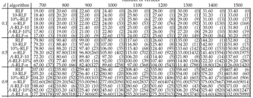
700, 800, . . . , 1500, and d = 0.1, 0.5, 0.9 are reported in Table 1. Each result is an average on 5 instances. We indicate the average number of colors produced by each algorithm, as well as the average computing times in seconds (shown in parenthesis), using a 3 GHz Intel Xeon X5675 machine with 8 GB of RAM. In Figure 4, we represent the evolution of the computing time (using an logarithmic
scale) for d= 0.5 and d = 0.9 when the number of vertices increases. The top curve
corresponds to 10−8mn2 = 10−8dn3(n− 1)/2, and indicates the expected shape of
0,1 1 10 100 1000 10000 100000 d=0.9 700 number of vertices 0,1 1 10 100 1000 10000 100000 700 1100 1500 number of vertices C
omputing times in sec
onds d=0.5 A-RLF-n A-RLF-10% A-RLF-10 RLF 1100 1500 10-8mn2 10-8mn2
Figure 4: Evolution of the computing time for random graphs.
We observe that the A-RLF-β algorithms are faster than the β-RLF ones, which
means that the construction of a stable set Cvfor a number M of vertices v increases
the computing time by a factor smaller than M. But the increase is real and makes the A-RLF-10% and A-RLF-n less attractive for large graphs. For example, while
RLF finds a coloring of R1500,0.9in 6 seconds, about 100 minutes are needed by
A-RLF-n. But the number of colors is reduced from 407.4 to 332, which represents
a gain of 18%. For comparison, applying the RLF algorithm n= 1500 times on
the same graph (i.e., using n-RLF) decreases the number of colors by only 7 units. These absolute and relative (in percent) gains in colors of the A-RLF-β and β-RLF
algorithms with respect to the standard RLF are shown in Figure 5 for d= 0.5 and
0.9. Similar curves can be obtained by comparing B-RLF-β with β-RLF. We clearly
observe that the alternative selection rules (i.e., parameterβ) for the first vertex
of a color class have very positive impact on the performance of the RLF algorithm.
number of vertices d algorithm 700 800 900 1000 1100 1200 1300 1400 1500 RLF 19.00 (0) 20.60 (0) 22.60 (0) 24.40 (0) 26.00 (0) 28.00 (0) 30.00 (0) 31.60 (0) 33.40 (0) 10-RLF 18.40 (0) 20.20 (0) 22.00 (0) 24.00 (0) 25.80 (1) 27.60 (1) 29.20 (1) 31.20 (1) 33.00 (1) 10%-RLF 18.00 (1) 20.00 (1) 22.00 (2) 24.00 (3) 25.80 (6) 27.00 (8) 29.00 (9) 31.00 (13) 33.00 (17) 0.1 n-RLF 18.00 (8) 20.00 (13) 22.00 (22) 24.00 (33) 25.80 (53) 27.00 (76) 29.00 (92) 31.00 (130) 32.80 (168) A-RLF-10 18.00 (0) 19.60 (0) 21.40 (0) 23.20 (0) 25.00 (0) 26.60 (0) 28.00 (1) 30.00 (1) 31.80 (1) A-RLF-10% 17.80 (1) 19.00 (1) 21.00 (1) 22.80 (2) 24.00 (3) 26.00 (5) 27.20 (8) 29.20 (10) 30.80 (19) A-RLF-n 17.00 (3) 19.00 (6) 21.00 (9) 22.60 (15) 24.00 (23) 25.60 (31) 27.00 (49) 29.00 (84) 30.20 (93) RLF 79.80 (0) 90.40 (0) 99.00 (0) 107.80 (1) 117.60 (1) 126.60 (1) 135.00 (2) 144.20 (1) 152.80 (2) 10-RLF 79.20 (1) 88.40 (1) 97.60 (3) 107.00 (3) 116.80 (6) 125.40 (8) 134.20 (11) 142.80 (11) 151.80 (15) 10%-RLF 78.80 (6) 88.20 (12) 97.40 (23) 106.00 (35) 115.40 (68) 124.40 (95) 133.60 (142) 142.00 (153) 150.80 (204) 0.5 n-RLF 78.20 (62) 87.80(118) 96.80(260) 105.80 (402) 115.00 (702) 123.60 (922) 133.00(1432) 141.40(1554) 150.00(1975) A-RLF-10 72.20 (1) 80.60 (1) 89.40 (2) 97.20 (3) 106.20 (4) 114.40 (5) 121.80 (8) 130.40 (14) 137.60 (17) A-RLF-10% 69.00 (5) 77.40 (9) 85.00 (16) 92.00 (33) 100.00 (39) 107.40 (69) 114.80 (106) 122.20 (142) 129.20 (280) A-RLF-n 67.00 (37) 75.00 (66) 82.40(127) 89.60 (258) 97.00 (368) 104.00 (543) 111.40 (788) 118.80(1261) 126.00(1420) RLF 207.00 (1) 235.80 (1) 259.40 (1) 286.40 (2) 308.40 (2) 335.80 (3) 358.60 (5) 382.60 (5) 407.40 (6) 10-RLF 205.20 (4) 230.80 (7) 256.40 (12) 280.80 (20) 306.00 (25) 331.00 (33) 354.00 (45) 379.20 (51) 403.80 (60) 10%-RLF 204.20 (28) 230.00 (52) 255.00(103) 279.60 (193) 303.60 (259) 328.80 (406) 352.40 (603) 376.40 (710) 400.60 (906) 0.9 n-RLF 202.60(280) 229.20(542) 253.00(961) 277.00(2050) 302.60(2837) 327.60(4074) 351.00(5757) 375.00(7667) 398.60(9014) A-RLF-10 188.60 (4) 210.80 (6) 233.20 (10) 255.60 (13) 280.60 (20) 301.60 (25) 325.80 (43) 346.80 (50) 371.00 (63) A-RLF-10% 182.00 (22) 203.20 (43) 225.40 (90) 245.60 (138) 267.20 (254) 287.00 (315) 306.20 (554) 325.40 (820) 343.80(1247) A-RLF-n 177.20(178) 197.80(318) 217.80(605) 236.60(1126) 255.20(1681) 275.20(2315) 294.20(3740) 314.60(4280) 332.00(5999)
Table 1:Comparison of the A-RLF-β and β-RLF algorithms on random graphs.
We have tested the eight versions of theα-RLF-β algorithm on the DIMACS
benchmark graph coloring instances that come from various sources. For a de-tailed description of these instances, the reader can refer to [20]. We only report results for the seemingly most challenging instances, those for which the DSATUR algorithm is not able to produce a coloring with k colors, where k is the best known
upper bound onχ(G). This gives a total of 63 instances with 36 ≤ n ≤ 10, 000
and 290≤ m ≤ 990, 000. Two measures are used to analyze the performances of
0 10 20 30 40 50 60 70 80 d=0.9 0 2 4 6 8 10 12 14 16 18 20 0 5 10 15 20 25 30 d=0.5 700 1100 1500 700 1100 1500 700 1100 1500 700 1100 1500 0 2 4 6 8 10 12 14 16 18 20 d=0.5
number of vertices number of vertices
number of vertices number of vertices
d=0.9 A-RLF-n A-RLF-10% A-RLF-10 n-RLF 10%-RLF 10-RLF A bsolut e gain A bsolut e gain R ela tiv e gain R ela tiv e gain
Figure 5: Color gains of the A-RLF-β and β-RLF algorithms with respect to RLF on random graphs.
the best known results. More precisely, for a set S of instances, let bsbe the best
known upper bound on the chromatic number of s∈ S, and let asbe the number
of colors produced by one of the algorithms. The TAPD of this algorithm is then defined as follows :
TAPD= 100
∑
s∈S∑(as− bs) s∈Sbs .
This measures gives more importance to results on graphs with a large number
of colors. For example, assume that there are only two instances s1 and s2 in S
with bs1 = 10 and bs2 = 100. If an algorithm Algo1 finds a coloring of s1 with
11 colors and a coloring of s2 with 100 colors, then its TAPD is 100110 = 0.909. If
a second algorithms Algo2 finds as1 = 10 and as2 = 110, then its TAPD is 10
times larger, which means that Algo1could appear to be better than Algo2. Both
algorithms have, however, similar results since they have reached the best known upper bound on one of the two instances, and produced a coloring with 10% more colors then the best known upper bound on the other instance. To compensate such a bias, we also compute the average relative percent deviation (ARPD) which is defined as follows : ARPD= 100 | S | ∑ s∈S as− bs bs .
For the above example, both algorithms Algo1and Algo2have an ARPD of 5.
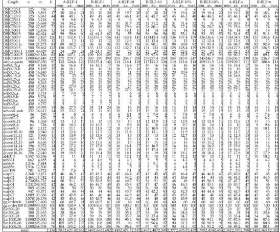
in Table 2. Each line in the table corresponds to a particular graph. The first columns indicate the name, the number of vertices, and the number of edges of the considered graph. The next column displays the best known upper bound k
on the chromatic number. Note that all versions of theα-RLF-β algorithm possibly
make random choices when choosing a first vertex v for a color class Cv, or the
next vertices to be added to Cv. Such choices occur when ties cannot be broken by
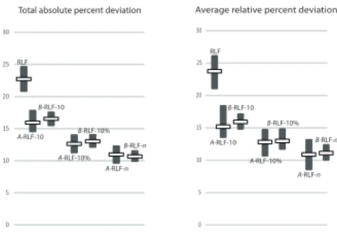
the proposed selections rules. Each algorithm was therefore run 10 times, and we report the minimum (column min), the average (column av.) and the maximum (column max) numbers of colors used by each version of the algorithm. The last line of table 2 indicates the total number of colors for the 63 instances. In Figure 6, we indicate the TAPDs and ARPDs associated with the best, average and the worst results of each algorithm.
Graph n m k A-RLF-1 B-RLF-1 A-RLF-10 B-RLF-10 A-RLF-10% B-RLF-10% A-RLF-n B-RLF-n min av. max min av. max min av. max min av. max min av. max min av. max min av. max min av. max DSJC125.1 125 736 5 6 6 6 6 6 6 6 6 6 6 6 6 6 6 6 6 6 6 6 6.2 7 6 6 6 DSJC125.5 125 3,891 17 20 20.4 21 20 20 20 19 19.7 20 20 20 20 19 19.4 20 19 19.4 20 19 19.1 20 18 18.4 19 DSJC125.9 125 6,961 44 48 49.1 50 49 49 49 45 46.1 47 45 45.7 47 45 46.3 48 46 46.5 47 45 46.1 47 45 45.8 46 DSJC250.1 250 3,218 8 9 9.8 10 9 9.3 10 9 9 9 9 9 9 9 9 9 9 9 9 9 9 9 9 9 9 DSJC250.5 250 15,668 28 34 34.2 35 36 36 36 31 31.7 32 31 31.2 32 31 31.4 32 31 31 31 , 30 30.9 31 31 31 31 DSJC250.9 250 27,897 72 83 83.6 85 85 85 85 78 79.6 81 78 80.1 82 76 77.4 79 78 78.7 80 75 75.8 77 75 76 77 DSJC500.1 500 12,458 12 14 14.8 15 15 15 15 14 14.1 15 14 14 14 14 14 14 14 14 14 14 14 14 14 14 14 DSJC500.5 500 62,624 48 59 59.6 60 61 61.3 62 54 55 56 56 56 56 52 53.1 54 53 53 53 51 51.8 52 51 51.1 52 DSJC500.9 500112,437 126 151 152.8 155 155155.1 156 143 143.4 145 141143.4 145 136 137.4 139 136136.6 138 134134.9 136 133 134.6 136 DSJR500.1 500 3,555 12 12 13 14 12 12 12 12 12.5 13 12 12.4 13 13 13 13 12 12.4 13 12 12.8 13 13 13 13 DSJR500.1c 500121,275 84 89 90.2 92 96 96 96 91 93.3 96 90 90.1 91 90 90.8 92 91 91.4 92 96 96.7 98 92 92.9 94 DSJR500.5 500 58,862 122 130 131.7 133 133 133 133 132 132.7 134 131 133 134 128 128.4 129 129130.5 131 126127.5 128 125 126.5 128 DSJC1000.1 1,000 49,629 20 24 24 24 24 24.1 25 23 23 23 23 23 23 22 22.6 23 23 23 23 22 22.1 23 22 22 22 DSJC1000.5 1,000249,826 83 106 107.1 108 109 109 109 96 97 98 97 97.9 99 92 92.5 93 92 92.9 93 90 90.3 91 89 89.1 90 DSJC1000.9 1,000449,449 222 275 279.7 283 290 290 290 255 256.7 258 255257.4 259 244 245.9 247 245246.7 248 236236.7 238 236 236.7 238 latin square 900307,350 97 122 124.6 129 132135.4 140 114 116.1 118 117121.3 126 110 111.6 114 109111.5 114 109109.7 111 107 108.6 111 le450 15 a 450 8,168 15 16 16.4 17 16 16.1 17 16 16.4 17 16 16 16 16 16 16 16 16 16 16 16.4 17 16 16 16 le450 15 b 450 8,169 15 16 16.1 17 16 16 16 16 16 16 16 16 16 16 16 16 16 16 16 16 16 16 16 16 16 le450 15 c 450 16,680 15 23 23.1 24 23 23 23 21 21 21 21 21 21 20 20.9 21 21 21 21 18 18.7 19 20 20 20 le450 15 d 450 16,750 15 23 23 23 23 23 23 22 22 22 22 22 22 21 21 21 21 21 21 18 18.8 19 19 19 19 le450 25 a 450 8,260 25 25 25 25 25 25 25 25 25 25 25 25 25 25 25 25 25 25 25 25 25 25 25 25 25 le450 25 b 450 8,263 25 25 25 25 25 25 25 25 25 25 25 25 25 25 25 25 25 25 25 25 25 25 25 25 25 le450 25 c 450 17,343 25 27 27.9 28 28 28 28 27 27 27 28 28 28 27 27 27 28 28 28 26 26.7 27 27 27 27 le450 25 d 450 17,425 25 28 28.1 29 29 29 29 27 27.2 28 27 27 27 27 27 27 27 27 27 27 27.3 28 27 27 27 le450 5 a 450 5,714 5 7 7.9 8 7 7 7 6 6 6 6 6 6 6 6 6 5 5 5 5 5 5 5 5 5 le450 5 b 450 5,734 5 7 7 7 7 7 7 5 5 5 5 5 5 5 5 5 5 5 5 5 5 5 5 5 5 le450 5 c 450 9,803 5 5 5 5 6 6 6 5 5 5 5 5 5 5 5 5 5 5 5 5 5 5 5 5 5 le450 5 d 450 9,757 5 5 5 5 7 7 7 5 5 5 5 5 5 5 5 5 5 5 5 5 5 5 5 5 5 school1 385 19,095 14 26 27.3 28 24 24 24 16 16 16 16 16 16 14 14 14 14 14 14 14 14 14 14 14 14 school1 nsh 352 14,612 14 22 23.2 24 21 21 21 15 15 15 15 15 15 15 15 15 15 15 15 15 15 15 15 15 15 queen6 6 36 290 7 8 8 8 8 8 8 8 8.1 9 7 7.9 8 7 7.8 8 7 7.8 8 8 8 8 7 7.6 8 queen7 7 49 476 7 9 9.2 10 9 9 9 7 7.2 9 7 7 7 8 8.9 9 7 8 10 7 7 7 7 8.2 9 queen8 12 96 1,368 12 13 13 13 13 13 13 13 13 13 12 12.9 13 12 12.9 14 12 12.9 13 12 12.8 13 13 13 13 queen8 8 64 728 9 10 10.3 11 10 10.3 11 9 9.9 10 10 10 10 9 9.7 10 10 10 10 10 10 10 9 9.6 10 queen9 9 81 2,112 10 11 11.1 12 11 11.8 12 10 10.7 11 10 10.9 11 10 10.4 11 10 10.5 11 10 10.7 11 10 10.1 11 queen10 10 100 2,940 11 12 12.6 13 12 12.2 13 11 11.8 13 12 12.1 13 11 11.9 13 12 12.1 13 11 11.7 12 12 12 12 queen11 11 121 3,960 11 13 13.9 14 13 13.9 14 13 13 13 13 13 13 12 12.7 13 13 13 13 12 12.3 13 13 13 13 queen12 12 144 5,192 12 14 14.9 15 15 15 15 14 14 14 14 14 14 14 14 14 14 14.1 15 13 13.6 14 14 14 14 queen13 13 169 6,656 13 15 15.9 16 15 15.8 16 15 15 15 15 15 15 15 15 15 15 15.2 16 14 14.9 15 14 14 14 queen14 14 196 8,372 14 17 17.2 18 17 17.8 18 16 16.1 17 16 16.5 17 16 16 16 16 16.2 17 15 15.8 16 16 16 16 queen15 15 225 10,360 15 17 18.2 19 19 19 19 17 17.1 18 17 17.4 18 17 17 17 17 17.1 18 16 16.6 17 17 17 17 queen16 16 256 12,640 16 19 19.5 20 19 19.4 20 18 18.1 19 18 19 20 18 18.1 19 18 18.4 19 17 17.8 18 17 17.9 18 abb313 1,557 53,356 9 11 11 11 11 11 11 12 12.1 13 10 10 10 11 11.2 12 10 10 10 11 11 11 10 10.2 11 ash331 662 4,185 4 4 4 4 4 4.8 5 4 4.3 5 5 5 5 4 4.2 5 4 4.3 5 4 4.2 5 4 4.2 5 ash608 1,216 7,844 4 5 5 5 5 5.2 6 4 4.2 5 5 5.1 6 4 4 4 5 5 5 4 4.2 5 5 5 5 ash958 1,916 12,506 4 5 5 5 5 5.2 6 5 5 5 5 5 5 4 4.8 5 5 5 5 4 4.8 5 5 5 5 will199 701 6,772 7 7 7.6 8 7 7 7 7 7.1 8 7 7 7 7 7 7 7 7 7 7 7.6 8 7 7 7 wap01 2,368110,871 42 46 46.3 47 45 45.2 46 45 46.4 47 45 45 45 45 46.4 47 46 46.8 47 45 45.8 47 45 45 45 wap02 2,464111,742 41 44 44.4 45 43 43.8 44 44 44.2 45 44 44 44 43 43.6 44 44 44 44 44 44.3 45 44 44.5 45 wap03 4,730286,722 44 50 51.1 52 50 50.8 52 48 49.7 51 51 51 51 48 49 51 49 50.3 51 47 47.7 49 51 51 51 wap04 5,231294,902 42 46 46.2 47 46 46.7 49 45 45.9 47 47 47 47 46 46.5 48 45 45.1 46 45 45.7 47 46 46 46 wap05 905 43,081 50 50 50 50 50 50 50 50 50 50 50 50 50 50 50 50 50 50 50 51 51 51 50 50 50 wap06 947 43,571 40 44 44 44 44 44 44 43 43.7 45 42 42.2 43 42 42.3 43 44 44.4 45 42 42.5 43 43 43 43 wap07 1,809103,368 42 45 45.8 47 46 46 46 44 44.9 46 45 45 45 45 45.5 46 46 46 46 45 45.4 46 45 45 45 wap08 1,870104,176 42 45 45.4 46 45 45.7 46 43 44.3 46 48 48 48 43 43.9 45 45 45 45 44 45.4 46 45 45 45 qg.order60 3,600212,400 60 60 60.7 61 60 60.5 61 60 60 60 60 60 60 60 60 60 60 60 60 60 60 60 60 60 60 qg.order10010,000990,000 100 100 100.9 101 100100.6 101 100 100.2 101 100 100 100 100 100 100 100 100 100 100 100 100 100 100 100 flat300 20 300 21,375 20 36 36.8 38 38 38 38 32 32.1 33 34 34 34 24 24 24 22 22 22 20 20 20 20 20 20 flat300 26 300 21,633 26 38 38.6 39 39 39 39 35 35.4 37 35 35 35 34 34.5 35 35 35 35 34 34 34 33 33.6 34 flat300 28 300 21,695 28 37 37.9 39 39 39 39 35 35.7 36 35 35.4 36 34 34.7 35 35 35 35 33 33.4 34 34 34 34 flat1000 50 1,000245,000 50 104 105.4 106 108 108 108 94 95.4 96 96 96.5 97 90 90.5 91 90 91.1 92 87 87.8 89 86 87.3 88 flat1000 60 1,000245,830 60 105 105.7 107 108 108 108 95 96 97 96 96.6 97 90 91.2 92 90 90.9 91 88 88.3 89 88 88.8 89 flat1000 76 1,000246,708 76 104 105.2 106 106 106 106 96 96.4 97 97 97 97 90 91.1 92 91 91.2 92 88 89.2 90 88 88.1 89 total 2,136 2,5812,621.42,662 2,6492,6632,682 2,4452,474.52,515 2,4652,4872,509 2,3772,405.52,435 2,3952,4142,436 2,3422,3702,398 2,3482,363.82,382
0 5 10 15 20 25 30 0 5 10 15 20 25 30
Total absolute percent deviation Average relative percent deviation
RLF A-RLF-10 B-RLF-10 A-RLF-10% B-RLF-10% A-RLF-n B-RLF-n RLF A-RLF-10 B-RLF-10 A-RLF-10% B-RLF-10% A-RLF-n B-RLF-n
Figure 6: Comparisons of theα-RLF-β algorithms on DIMACS benchmark instances.
For β = 1, we observe that the standard function A, proposed by Leighton,
produces better results than function B. The difference between the best and
the worst results is however much smaller withα = B than with α = A, which
indicates that the proposed alternative greedy choice is more stable. This becomes
even more evident withβ = 10. Indeed, while the best minimum and average
results are obtained with α = A, the best worst case comes with α = B. For
β = 10%, the difference in terms of total number of colors between the worst and
the best case withα = A is 58 (2435-2377) while this difference is equal to 41
(2436-2395) withα = B. Interestingly, by comparing the TAPDs, we observe that
A-RLF-n has better best case than B-RLF-n, but worse average and worst cases.
The gap between the total average number of colors produced by A-RLF-1 and the best known upper bound k is equal to 485.4 (2621.4-2136). This gap is reduced to 234 (2370-2136) with A-RLF-n, which represents an improvement of 51.8%. When comparing B-RLF-1 with B-RLF-n, the improvement is even larger since the difference between the total average number of colors and k is reduced from 527 (2663-2136) to 227.8 (2363.6-2136), which corresponds to an improvement of
56.8%. The majority of this improvement is already obtained by settingβ = 10
instead of 1. Indeed, the gain is of 30.3% for α = A and of 33.4% for α = B. The importance of modifying the greedy choices made in RLF is very clear on some instances. One of the best illustrations is given by instance school1 where the standard RLF algorithm uses 26 colors while A-RLF-10 and B-RLF-10 find colorings with only 16 colors. The best known upper bound for this instance is
14, and is reached withβ = 10% and β = n. Another good example is instance
flat300 20 where the best coloring produced by RLF uses 36 colors, while only 20 colors are used by A-RLF-n and B-RLF-n (which is the chromatic number of the considered graph). Note however that the standard RLF eventually produces better results than all proposed variations. For example, for instance DSJR500.1c, RLF uses 89 colors, while the best coloring obtained with all proposed alternatives contains 90 colors.
Graph n m RLF A-RLF-10 A-RLF-10% A-RLF-n DSJC125.1 125 736 0 0 0 0 DSJC125.5 125 3,891 0 0 0 0 DSJC125.9 125 6,961 0 0 0 0 DSJC250.1 250 3,218 0 0 0 0 DSJC250.5 250 15,668 0 0 0 1 DSJC250.9 250 27,897 0 0 1 2 DSJC500.1 500 12,458 0 0 0 1 DSJC500.5 500 62,624 0 1 1 7 DSJC500.9 500 112,437 0 1 4 27 DSJR500.1 500 3,555 0 0 0 1 DSJR500.1c 500 121,275 0 1 2 11 DSJR500.5 500 58,862 0 1 2 13 DSJC1000.1 1,000 49,629 0 0 2 16 DSJC1000.5 1,000 249,826 0 3 35 283 DSJC1000.9 1,000 449,449 2 15 158 875 latin square 900 307,35 1 5 25 187 le450 15 a 450 8,168 0 0 0 1 le450 15 b 450 8,169 0 0 0 1 le450 15 c 450 16,680 0 1 0 1 le450 15 d 450 16,750 0 0 0 1 le450 25 a 450 8,260 0 0 1 1 le450 25 b 450 8,263 0 0 0 1 le450 25 c 450 17,343 0 0 0 2 le450 25 d 450 17,425 0 0 1 1 le450 5 a 450 5,714 0 0 0 1 le450 5 b 450 5,734 0 0 0 1 le450 5 c 450 9,803 0 0 0 0 le450 5 d 450 9,757 0 0 0 1 school1 385 19,095 0 0 0 1 school1 nsh 352 14,612 0 0 0 1 queen6 6 36 290 0 0 0 0 queen7 7 49 476 0 0 0 0 queen8 12 96 1,368 0 0 0 0 queen8 8 64 728 0 0 0 0 queen9 9 81 2,112 0 0 0 0 queen10 10 100 2,940 0 0 0 0 queen11 11 121 3,960 0 0 0 0 queen12 12 144 5,192 0 0 0 0 queen13 13 169 6,656 0 0 0 0 queen14 14 196 8,372 0 0 0 0 queen15 15 225 10,360 0 0 0 0 queen16 16 256 12,640 0 0 0 1 abb313 1,557 53,356 0 0 4 21 ash331 662 4,185 0 0 0 1 ash608 1,216 7,844 0 1 2 9 ash958 1,916 12,506 0 1 7 44 will199 701 6,772 0 0 1 1 wap01 2,368 110,871 1 4 64 454 wap02 2,464 111,742 1 4 82 590 wap03 4,730 286,722 2 16 643 5218 wap04 5,231 294,902 2 15 739 6208 wap05 905 43,081 0 0 2 15 wap06 947 43,571 0 1 3 16 wap07 1,809 103,368 1 2 26 201 wap08 1,870 104,176 1 2 27 195 qg.order60 3,600 212,400 2 11 501 2899 qg.order100 10,000 990,000 16 130 17330 91064 flat300 20 300 21,375 0 0 1 1 flat300 26 300 21,633 0 0 0 1 flat300 28 300 21,695 0 0 0 1 flat1000 50 1,000 245,000 1 4 34 178 flat1000 60 1,000 245,830 1 4 35 177 flat1000 76 1,000 246,708 1 5 36 179
Table 3: Average computing times (in seconds) of the A-RLF-β algorithms on DIMACS
β = 1 β = 10 β = 10% β = n
Graph n m k DS min av. max min av. max min av. max min av. max ST DSJC125.1 125 736 5 6 6 6 6 6 6 6 6 6 6 6 6 6 5 DSJC125.5 125 3,891 17 21 20 20 20 19 19.7 20 19 19.4 20 18.4 18 19 17 DSJC125.9 125 6,961 44 50 48 48.8 49 45 45.5 46 45 46.2 47 45.8 45 46 44 DSJC250.1 250 3,218 8 10 9 9.1 10 9 9 9 9 9 9 9 9 9 8 DSJC250.5 250 15,668 28 38 34 34.2 35 31 31.2 32 31 31 31 30.9 30 31 29 DSJC250.9 250 27,897 72 91 83 83.6 85 78 79.5 80 76 77.4 79 75.6 75 76 72 DSJC500.1 500 12,458 12 16 14 14.8 15 14 14 14 14 14 14 14 14 14 13 DSJC500.5 500 62,624 48 67 59 59.6 60 54 55 56 52 52.9 53 51 51 51 50 DSJC500.9 500 112,437 126 161 151 152.8 155 141 142.8 143 136 136.6 138 134.4 133 136 130 DSJR500.1 500 3,555 12 12 12 12 12 12 12.4 13 12 12.4 13 12.8 12 13 12 DSJR500.1c 500 121,275 84 87 89 90.2 92 90 90.1 91 90 90.7 91 92.9 92 94 86 DSJR500.5 500 58,862 122 130 130 131.7 133 131 132.5 134 128 128.4 129 126.4 125 128 128 DSJC1000.1 1,000 49,629 20 26 24 24 24 23 23 23 22 22.6 23 22 22 22 22 DSJC1000.5 1,000 249,826 83 114 106 107.1 108 96 97 98 92 92.5 93 89.1 89 90 89 DSJC1000.9 1,000 449,449 222 297 275 279.7 283 255 256.5 258 244 245.7 247 236.7 236 238 245 latin square 900 307,350 97 126 122 124.6 129 114 116.1 118 109 111.4 114 108.4 107 110 106 le450 15 a 450 8,168 15 16 16 16.1 17 16 16 16 16 16 16 16 16 16 15 le450 15 b 450 8,169 15 16 16 16 16 16 16 16 16 16 16 16 16 16 15 le450 15 c 450 16,680 15 24 23 23 23 21 21 21 20 20.9 21 18.7 18 19 16 le450 15 d 450 16,750 15 24 23 23 23 22 22 22 21 21 21 18.8 18 19 16 le450 25 a 450 8,260 25 25 25 25 25 25 25 25 25 25 25 25 25 25 25 le450 25 b 450 8,263 25 25 25 25 25 25 25 25 25 25 25 25 25 25 25 le450 25 c 450 17,343 25 29 27 27.9 28 27 27 27 27 27 27 26.7 26 27 27 le450 25 d 450 17,425 25 28 28 28.1 29 27 27 27 27 27 27 27 27 27 27 le450 5 a 450 5,714 5 10 7 7 7 6 6 6 5 5 5 5 5 5 5 le450 5 b 450 5,734 5 9 7 7 7 5 5 5 5 5 5 5 5 5 5 le450 5 c 450 9,803 5 6 5 5 5 5 5 5 5 5 5 5 5 5 5 le450 5 d 450 9,757 5 11 5 5 5 5 5 5 5 5 5 5 5 5 5 school1 385 19,095 14 17 24 24 24 16 16 16 14 14 14 14 14 14 14 school1 nsh 352 14,612 14 25 21 21 21 15 15 15 15 15 15 15 15 15 14 queen6 6 36 290 7 9 8 8 8 7 7.9 8 7 7.7 8 7.6 7 8 7 queen7 7 49 476 7 10 9 9 9 7 7 7 7 7.8 9 7 7 7 7 queen8 12 96 1,368 12 13 13 13 13 12 12.9 13 12 12.7 13 12.8 12 13 12 queen8 8 64 728 9 12 10 10.1 11 9 9.9 10 9 9.7 10 9.6 9 10 9 queen9 9 81 2,112 10 14 11 11 11 10 10.7 11 10 10 10 10 10 10 10 queen10 10 100 2,940 11 13 12 12.2 13 11 11.7 12 11 11.8 12 11.7 11 12 11 queen11 11 121 3,960 11 15 13 13.8 14 13 13 13 12 12.7 13 12.3 12 13 11 queen12 12 144 5,192 12 15 14 14.9 15 14 14 14 14 14 14 13.6 13 14 13 queen13 13 169 6,656 13 17 15 15.7 16 15 15 15 15 15 15 14 14 14 14 queen14 14 196 8,372 14 18 17 17.2 18 16 16 16 16 16 16 15.8 15 16 15 queen15 15 225 10,360 15 19 17 18.2 19 17 17 17 17 17 17 16.6 16 17 16 queen16 16 256 12,640 16 21 19 19.2 20 18 18 18 18 18 18 17.8 17 18 17 abb313 1,557 53,356 9 11 11 11 11 10 10 10 10 10 10 10.2 10 11 11 ash331 662 4,185 4 5 4 4 4 4 4.3 5 4 4 4 4.2 4 5 5 ash608 1,216 7,844 4 5 5 5 5 4 4.2 5 4 4 4 4.2 4 5 5 ash958 1,916 12,506 4 6 5 5 5 5 5 5 4 4.8 5 4.8 4 5 6 will199 701 6,772 7 7 7 7 7 7 7 7 7 7 7 7 7 7 7 wap01 2,368 110,871 42 46 45 45.2 46 45 45 45 45 46.3 47 45 45 45 45 wap02 2,464 111,742 41 45 43 43.8 44 44 44 44 43 43.6 44 44 44 44 44 wap03 4,730 286,722 44 54 50 50.7 51 48 49.7 51 48 49 51 47.7 47 49 53 wap04 5,231 294,902 42 48 46 46 46 45 45.9 47 45 45.1 46 45.6 45 46 48 wap05 905 43,081 50 50 50 50 50 50 50 50 50 50 50 50 50 50 50 wap06 947 43,571 40 46 44 44 44 42 42.2 43 42 42.3 43 42.5 42 43 44 wap07 1,809 103,368 42 46 45 45.7 46 44 44.7 45 45 45.5 46 45 45 45 45 wap08 1,870 104,176 42 45 45 45.4 46 43 44.3 46 43 43.9 45 44.9 44 45 45 qg.order60 3,600 212,400 60 62 60 60.3 61 60 60 60 60 60 60 60 60 60 60 qg.order100 10,000 990,000 100 103 100 100.6 101 100 100 100 100 100 100 100 100 100 100 flat300 20 300 21,375 20 40 36 36.8 38 32 32.1 33 22 22 22 20 20 20 20 flat300 26 300 21,633 26 41 38 38.6 39 35 35 35 34 34.5 35 33.6 33 34 27 flat300 28 300 21,695 28 41 37 37.9 39 35 35.4 36 34 34.7 35 33.4 33 34 31 flat1000 50 1,000 245,000 50 112 104 105.4 106 94 95.4 96 90 90.5 91 87.3 86 88 92 flat1000 60 1,000 245,830 60 113 105 105.7 107 95 95.8 96 90 90.9 91 88.1 88 89 93 flat1000 76 1,000 246,708 76 114 104 105.2 106 96 96.4 97 90 90.9 91 88 88 88 88 total 2,136 2,733 2,576 2,606.9 2,64 2,436 2,460.8 2,482 2,369 2,394.5 2,416 2,326 2,349.9 2,371 2,331
It is important to mention that the improvement in quality obtained by using β = 10% or β = n instead of β = 1 or β = 10 has a price. Indeed, we report in Table 3 the average computing times of the A-RLF-β algorithms (similar times are needed by the B-RLF-β algorithms). For example, for instance DSJC1000.9, the best coloring produced by RLF uses 275 colors and is obtained in 2 seconds, while only 236 colors are used by A-RLF-n, such a coloring being obtained in about 14 minutes. Also, the optimal coloring in 100 colors of instance qg.order100 is obtained by RLF in 16 seconds, while 15 hours are needed by A-RLF-n, and 5 hours by A-RLF-10%. But for instances of a reasonable size like flat300 20, the reduction from 36 to 20 colors mentioned above is obtained in one second. Also, for instance school1, one second is sufficient to reduce the number of used colors from 26 to 14. It is also interesting to observe that while A-RLF-n and B-RLF-n show similar behaviors, they produce very different results on some instances. For example,
B-RLF-n is able to find a coloring with 92 colors for DSJR500.1c while the best
coloring produced by A-RLF-n for this instance contains 4 additional colors. On the opposite, the best coloring produced by B-RLF-n for wap03 has 51 colors, while colorings with only 47 colors were found by A-RLF-n. In summary, the two algorithms seem complementary, which explains why we now report results obtained by running both A-RLF-β and B-RLF-β, and keeping only the best of the two produced colorings. This new algorithm, called AB-RLF-β is compared to DSATUR [1] and to the Short Tabu algorithm studied in [8], which consists in taking the best result of 5 runs with 100,000 iterations of the TABUCOL algorithm of Hertz and de Werra [13]. Comparisons between these algorithms are shown in Table 4, while their TAPDs and ARPDs appear in Figure 7. The first four columns of Table 4 are the same as those in Table 2. The next columns display the best result produced by DSATUR (column DS), the minimum, average and maximum numbers of colors used by each version of the AB-RLF-β algorithm, and finally the best result produced by Short Tabu (column ST). The last line of Table 4 shows totals on the 63 instances. We observe that while the best total
number of colors used byα-RLF-n is 2342 for α = A and 2348 for α = B (see Table
2), it is reduced to 2326 by AB-RLF-n, which is even better than the total of 2331 colors produced by Short Tabu. The best TAPDs and ARPDs of the AB-RLF-β algorithms, as well as those of DSATUR, RLF and Short Tabu are shown in Figure 8. We see, for example, that while DSATUR has a TAPD of 27.95%, the standard RLF reduces it to 20.8%, and the AB-RLF-n algorithm to 8.9%, which corresponds to an additional gain of 11.9%. A perfect illustration of the effectiveness of the proposed algorithms is given by instance DSJC1000.9. The DSATUR algorithm finds a coloring with 297 colors, while only 275 are necessary with RLF. With α-RLF-n, we were able to gain 39 (275-236) additional colors, which is 6 units better than the result produced by Short Tabu. The coloring with 236 colors that we have obtained is however 14 units above the best results produced by more complex and more time-consuming metaheuristics.
Short_Tabu 0 5 10 15 20 25 30 Short_Tabu
Total absolute percent deviation Average relative percent deviation
0 5 10 15 20 25 30 35 DSATUR DSATUR RLF RLF AB-RLF-1 AB-RLF-1 AB-RLF-10 AB-RLF-10 AB-RLF-10% AB-RLF-10% AB-RLF-n AB-RLF-n
Figure 7: Comparisons of the AB-RLF-β algorithms on DIMACS benchmark instances.
0 5 10 15 20 25 30 35
DSATUR RLF AB-RLF-1 AB-RLF-10 AB-RLF10% AB-RLF-n Short_Tabu
TAPD ARPD 27.95 20.83 20.60 14.04 10.91 8.90 9.13 31.75 23.59 20.66 12.75 9.63 7.61 7.84
Figure 8: Some TAPDs and ARPDs for the DIMACS benchmark instances.
5. CONCLUSION
The RLF algorithm is a very popular heuristic for the vertex coloring problem, mainly because it is easy to implement and has a relatively low complexity in
O(mn). Since various greedy choices made in RLF can have a very big impact
on the performance of the algorithm, we have proposed alternative choices. Ex-periments have shown that much better colorings can be obtained with these
alternative greedy choices. The proposed AB-RLF-n algorithm has an O(mn2)
complexity, and competes with basic metaheuristics like Short Tabu. The differ-ence between the number of colors used and the best known upper bound is, on average, reduced by more than 50% when compared with the standard RLF. More than 30% of this improvement can be obtained with AB-RLF-10 which is an O(mn) algorithm, like RLF. By implementing the different versions of our algorithms, we have not sought to optimize the code, our goal being rather to demonstrate the quality gain that can be achieved by modifying the greedy choices made in the standard RLF algorithm. Better implementations based on the same ideas as those presented in [5] would certainly lead to faster algorithms. We finally note that the AB-RLF-n algorithm is a perfect candidate for a parallel implementation since
each color class is obtained by choosing among different stable sets Cv (one for
every uncolored vertex v), and these stable sets can be generated independently by different processors.
REFERENCES
[1] Br´elaz, D., “New methods to color the vertices of a graph”, Communications of the ACM, 22 (1979) 251–256.
[2] Brown, J.R., “Chromatic scheduling and the chromatic number problem”, Management Science, 19 (1972) 456–463.
[3] Chams, M., Hertz, A., de Werra, D., “Some experiments with simulated annealing for coloring graphs”, European Journal of Operational Research, 32 (1987) 260–266.
[4] Garey, M., Johnson, D.S., Computer and Intractability, Freeman, San Francisco, 1979.
[5] Chiarandini, M., Galbiati, G., Gualandi, S., “Efficiency issues in the RLF heuristic for graph coloring”, Proceedings of the IX Metaheuristics International Conference, (MIC 2011), July 2011, Udine, Italy, 461–469.
[6] Chiarandini, M., Gualandi, S., http://www.imada.sdu.dk/∼marco/gcp/
[7] Chiarandini, M., Stuetzle, T., “An analysis of heuristics for vertex colouring”, Lecture Notes in
Computer Science, 6049 (2010) 326–337.
[8] Galinier, P., Hertz, A., Zufferey, N., “An adaptive Memory Algorithm for the k-Colouring Prob-lem”, Discrete Applied Mathematics, 156 (2008) 267–279.
[9] Gualandi, S., Malucelli, F., “Exact Solution of Graph Coloring Problems via Constraint Program-ming and Column Generation”, INFORMS Journal on Computing, 24 (2012) 81–100.
[10] Halld ´orsson, M., “A still better performance guarantee for approximate graph coloring”,
Infor-mation Processing Letters, 45 (1993) 19–23.
[11] Held, S., Cook, W., Sewell, E.C., “Maximum-weight stable sets and safe lower bounds for graph coloring”, Mathematical Programming Computation, 4 (2012) 363–381.
[12] Herrmann, F., Hertz, A., “Finding the chromatic number by means of critical graphs”, ACM
Journal of Experimental Algorithmics, 7 (2002) 1–9.
[13] Hertz, A., de Werra, D., “Using tabu search techniques for graph coloring”, Computing, 39 (1987) 345–351.
[14] Johnson, D.S., Aragon, C.R., McGeoch, L.A., Shevon, C., “Optimization by simulated annealing: an experimental evalutation; part II, graph coloring and number partitioning”, Operations Research, 39 (1991) 378–406.
[15] Kubale, M., Jackowski, B., “A generalized implicit enumeration algorithm for graph coloring”,
Communications of the ACM, 28 (1985) 412–418.
[16] Leighton, F.T., “A graph coloring algorithm for large scheduling problems”, Journal of Research
of the National Bureau of Standards, 84 (1979) 489–503.
[17] Malaguti, E., Monaci, M., Toth, P., “An Exact Approach for the Vertex Coloring Problem”, Discrete Optimization, 8 (2) (2011) 174–190.
[18] Mehrotra, A., Trick, M.A., “A column generation approach for exact graph coloring”, INFORMS
Journal on Computing, 8 (1996) 344–354.
[19] Peem ¨oller, J., “A correction to Br´elaz’s modification of Brown’s coloring algorithm”,
Communi-cations of the ACM, 26 (1983) 593–597.