A dynamic model of parrotfish (family: Scaridae) populations for the management of herbivory on Caribbean coral reefs

HAL Id: dumas-00906910

https://dumas.ccsd.cnrs.fr/dumas-00906910

Submitted on 20 Nov 2013

HAL is a multi-disciplinary open access archive for the deposit and dissemination of sci-entific research documents, whether they are pub-lished or not. The documents may come from teaching and research institutions in France or abroad, or from public or private research centers.

L’archive ouverte pluridisciplinaire HAL, est destinée au dépôt et à la diffusion de documents scientifiques de niveau recherche, publiés ou non, émanant des établissements d’enseignement et de recherche français ou étrangers, des laboratoires publics ou privés.

A dynamic model of parrotfish (family: Scaridae)

populations for the management of herbivory on

Caribbean coral reefs

Caroline Baille

To cite this version:

Caroline Baille. A dynamic model of parrotfish (family: Scaridae) populations for the management of herbivory on Caribbean coral reefs. Sciences agricoles. 2013. �dumas-00906910�

i

Mémoire de fin d’Etudes

Diplôme d’Ingénieur de l’Institut Supérieur des Sciences

Agronomiques, Agroalimentaires, Horticoles et du Paysage

Année universitaire : 2012-2013

Spécialisation Halieutique - Option Ressources et Ecosystèmes Aquatiques

A dynamic model of parrotfish (family: Scaridae) populations for the management of herbivory on Caribbean coral reefs

Par : Caroline BAILLE

Sparisoma viride

Volet à renseigner par l’enseignant responsable de spécialisation ou son représentant Bon pour dépôt (version définitive) 

Date ; …./…/…

Autorisation de diffusion : Oui  Non

Signature :

Soutenu à Brisbane, en visioconférence avec Rennes le 11 Septembre 2013 Devant le jury :

Sous la présidence de : Didier GASCUEL

Maîtres de stage: Yves-Marie BOZEC and Shay O’FARRELL, University of Queensland, Enseignant référent : Didier GASCUEL, Agrocampus Ouest

Autres membres du jury : Etienne RIVOT, Agrocampus Ouest; Marianne ROBERT, IFREMER

AGROCAMPUS OUEST CFR Rennes

65, rue de Saint Brieuc 35000 RENNES

Marine Spatial Ecology Lab

School of Biological Sciences University of Queensland

St Lucia

Brisbane QLD 4072, Australia

"Les analyses et les conclusions de ce travail d'étudiant n'engagent que la responsabilité de son auteur et non celle d’AGROCAMPUS OUEST".

ii

Fiche de diffusion du mémoire

A remplir par l’auteur(1)

avec le maître de stage.

Aucune confidentialité ne sera prise en compte si la durée n’en est pas précisée.

Préciser les limites de la confidentialité (2) :

 Confidentialité absolue :  oui  non

(ni consultation, ni prêt)

 Si oui 1 an 5 ans 10 ans

 A l’issue de la période de confidentialité ou si le mémoire n’est pas confidentiel, merci de renseigner les éléments suivants :

Référence bibliographique diffusable(3) _:  oui  non

Résumé diffusable :  oui  non

Mémoire consultable sur place :  oui  non Reproduction autorisée du mémoire :  oui  non

Prêt autorisé du mémoire :  oui  non

……….

Diffusion de la version numérique :  oui  non  Si oui, l’auteur(1)

complète l’autorisation suivante :

Je soussignée Caroline BAILLE, propriétaire des droits de reproduction dudit résumé, autorise toutes les sources bibliographiques à le signaler et le publier.

Date : 2 Septembre 2013 Signature :

Rennes/Angers, le

Le maître de stage(4)_, L’auteur(1)_,

L’enseignant référent, (1) auteur = étudiant qui réalise son mémoire de fin d’études

(2) L’administration, les enseignants et les différents services de documentation d’AGROCAMPUS OUEST s’engagent à respecter cette confidentialité.

(3) La référence bibliographique (= Nom de l’auteur, titre du mémoire, année de soutenance, diplôme, spécialité et spécialisation/Option)) sera signalée dans les bases de données documentaires sans le résumé.

iii

Acknowledgment

First and foremost, I would like to thank Peter Mumby for welcoming me in his lab and

for his guidance throughout my project the past 5 months. I am really honoured to have

worked in his lab.

Bien évidemment un très grand merci à Yves-Marie pour avoir été mon maître stage de

fin d’études. Merci de m’avoir guidée et pour tout ce que j’ai appris. Merci pour ta

gentillesse et ta patience particulièrement dans les moments où je n’y croyais plus et

avant même le début du stage, durant le long processus d’obtention du visa. Merci pour

tout.

Huge thanks to my co-supervisor Shay for his support and for teaching me a lot about

parrotfish biology, and also for his continuous and precious encouragements during my

time at MSEL.

I would like to thank Dr. Jules van Rooij, Prof. John H. Choat and Dr. Halastair Harborne

for providing data for this study.

Many thanks to the “old” PhD students I shared the office with during 5 months: Alyssa,

Carolina, Elma, Jimena, Tries. Thank you for your good mood, for your support and

encouragements. I know it would have been much harder without you.

Thanks to Iliana for her very warm welcoming and help during my first days at MSEL and

for her incredible kindness.

Thanks to Alice, Chris B., Chris D., Juan, Sabah and everybody I met at MSEL. Thanks for

the good times.

Je tiens à remercier l’équipe du Pôle Halieutique d’Agrocampus Ouest pour leur soutien

et pour toutes les connaissances acquises en master 1 et 2.

Enfin, tendres et profonds remerciements à ma famille qui me soutient depuis toujours

et qui m’a aidée à y croire et ce, malgré les milliers de kilomètres qui souvent nous

séparent.

iv

Table of contents

Résumé ... v

List of Figures ... viii

List of Tables ... ix

Introduction ... 1

1. Material and Methods... 2

1.1. Animal study: Sparisoma viride (S. viride) biology ... 2

1.2. Available data on Sparisoma viride ... 4

1.2.1. Bonaire time series of abundance data ... 4

1.2.2. Growth data ... 4

1.2.3. Additional data ... 5

1.3. Model development ... 5

1.3.1. Choice of the type of model... 5

1.3.2. Model structure ... 6

1.3.3. Model parameterisation ... 7

1.3.4. Model implementation and outputs ... 10

1.4. Model calibration: population at equilibrium ... 12

1.4.1. Re-organisation of Bonaire data ... 12

1.4.2. Optimisation of model parameters ... 13

1.4.3. Exploration of the optimised model ... 14

1.4.4. Sensitivity analysis of the model to the parameters ... 14

1.5. Model application: recovery after applying fishing pressure ... 14

2. Results ... 15

2.1. Model construction: the Growth Transition Matrix ... 15

2.2. Optimisation results ... 17

2.3. Exploration of the model with optimised parameters ... 18

2.3.1. Model at equilibrium ... 18

2.3.2. Exploration of the behaviour of the optimised model ... 20

2.4. Sensitivity analysis: influence of the parameters on the size distribution ... 22

2.5. Recovery of the population after fishing disturbance ... 24

3. Discussion ... 24

3.1. Model structure and behaviour ... 25

3.1.1. Model structure ... 25 3.1.2. Model processes ... 25 3.1.3. Model optimisation ... 25 3.2. Model results ... 26 3.2.1. Growth ... 26 3.2.2. Recruitment ... 26

3.2.3. Size distribution at equilibrium... 26

3.3. Sensitivity analysis of the model ... 28

3.4. Recovery ater fishing disturbance ... 28

3.5. Future work with the model ... 29

v

Résumé

Les herbivores ont un rôle central pour la santé et la résilience des récifs coralliens. Aujourd'hui, le poisson perroquet est l’herbivore le plus important des Caraïbes et celui qui contribue le plus à maintenir des niveaux d’herbivorie fonctionnels sur les récifs coralliens en limitant la croissance et la colonisation des algues compétitrices des coraux (Hughes et

al., 2007). Sparisoma viride est l’une des espèces de poisson perroquet contribuant le plus au maintien de cette herbivorie fonctionnelle sur les récifs coralliens des Caraïbes (Mumby, 2006). Ces dernières années, la santé des récifs coralliens des Caraïbes s’est sévèrement

dégradée suite à une combinaison de perturbations d’origines naturelles et anthropiques, entrainant un changement de régime sur de nombreux récifs autrefois dominés par du corail vivant mais aujourd'hui dominés par les algues (Hughes 1994; Hughes et al., 2003). S. viride est la plus pêchée des espèces de poissons perroquets dans les Caraïbes (Mumby

et al., 2006). En perspective des changements globaux et de l’augmentation des

perturbations, le besoin est urgent de développer des outils de gestion à échelles locales pour la protection des poissons perroquet qui permettra le maintien de niveaux d’herbivorie fonctionnels. Pour implémenter des mesures de gestion efficaces, il est nécessaire d’avoir des connaissances sur la dynamique des poissons perroquets. Cependant, ces connaissances sont insuffisantes. La création d’un modèle de dynamique des populations de S. viride peut permettre d’améliorer ces connaissances en vue d’une mise en place de mesures de gestion telles que des quotas de pêche. Nous avons développé un modèle de dynamique des populations de S. viride structuré en tailles et catégories d’habitat. Ce modèle simule l’abondance de S. viride en fonction de la mortalité naturelle, de la croissance individuelle et du recrutement. Les catégories d’habitat des plus grands poissons sont basées sur la densité dépendance dans l’habitat profond du récif, inférée par un nombre limité de mâles matures dans cet habitat profond lié à la territorialité. Le modèle a été calibré avec une série temporelle d’abondance de S. viride collectée à Bonaire (Antilles Hollandaises). La population de S. viride de Bonaire possède une pression de pêche très faible et considérée comme étant à l’équilibre écologique. Le pas de temps choisi pour le modèle est de 3 mois pour concorder avec la fréquence de collecte des données à Bonaire. Avec ce modèle calibré, une pression de pêche a été simulée pour étudier la capacité du modèle à reproduire le rétablissement de la population de poissons perroquet observé aux Bermudes suite à la mise en place d’un moratoire sur l’utilisation des pièges à poissons.

Trois phases sont distinguables chez S. viride : la phase juvénile (J), la phase initiale (PI), individus femelles, et la phase terminale (PT), individus males. Les poissons perroquets sont des hermaphrodites et les femelles (PI) peuvent changer de sexe au cours de leur vie. La population de S. viride de l’île de Bonaire est organisée socialement et spatialement. Une zone de territoires est distinguable dans l’habitat profond du récif (>4m). Chaque territoire est mené par un mâle dominant (PT) et regroupe un harem de femelles. Dans l’habitat peu profond (<4m), les individus sont organisés sans structure particulière et constituent un simple groupe d’individus (J+PI+PT). Des individus mâles peuvent migrer de l’habitat peu profond vers un territoire pour prendre la place d’un mâle dominant lorsque celui-ci meurt ou émigre. Les femelles de l’habitat peu profond peuvent migrer également vers l’habitat profond pour devenir part du harem d’un TP mâle.

Nous disposions de plusieurs jeux de données pour cette étude. Nous avons calibré le modèle avec la série temporelle d’abondance de S. viride collectée à Bonaire par van Rooij

et al. (1996b) entre 1989 et 1992. Ces données ont été récoltées par comptage visuels et organisées par phases et taille des individus. Ces données ont permis de calibrer le modèle et d’estimer la valeur des paramètres à l’équilibre. Pour l’implémentation de la mortalité naturelle dans le modèle, nous avons testé 3 fonctions de mortalité: une mortalité constante selon la taille, une mortalité linéairement décroissante avec la taille et une mortalité exponentiellement décroissante avec la taille. Ces deux dernières fonctions supportent

vi

l’hypothèse que les poissons de plus petite taille sont plus vulnérables à la prédation et donc possèdent une mortalité supérieure à celle des poissons de plus grande taille. L’étape d’optimisation avec le solver Global Search de Matlab a été conduite en choisissant de minimiser la sommes des carrés des écarts entre les densités de classes de tailles observées à Bonaire et celles estimées par le modèle. L’optimisation n’a pas permis d’obtenir un meilleur fit aux données de Bonaire avec une fonction de mortalité dépendant de la taille. C’est donc la mortalité constante par classe de taille qui a été retenue pour étudier le modèle à l’équilibre. La croissance a été implémentée par une matrice de transition car le modèle est structuré en taille. Les entrées de cette matrice ont en particulier été calculées grâce aux données de correspondance taille-âge d’individus de S. viride communiquées par le Prof. John Howard Choat (School of Marine Biology and Aquaculture, James Cook University, Townsville, Australie) qui nous ont permis d’estimer les paramètres Linf et K de von Bertalanffy. Ces données ont été complétées par des données obtenues dans la base de données Fishbase. Le recrutement a été implémenté comme une addition constante de poissons de 5cm à chaque pas de temps. La valeur de recrutement estimée à l’étape d’optimisation a montré une valeur proche des valeurs de densités de poissons de même taille dans des sites du Belize et des Bahamas. Enfin, la densité dépendance a été implémentée pour recréer la limitation du nombre de territoires de l’habitat profond à Bonaire. Les migrations de poissons de l’habitat peu profond vers l’habitat profond ont été simulées par une simple limitation de la transition en fonction de la capacité limite de cet habitat profond.

Après un certain nombre de pas de temps, le modèle se stabilise à un état d’équilibre : les densités des classes de taille ne varient plus au cours du temps. La distribution de taille estimée par le modèle à l’équilibre a montré de fortes similitudes avec celle observée à Bonaire bien que les densités par classes de tailles soient globalement sous estimées. Le modèle calibré et à l’équilibre a permis de tester différentes hypothèses. (1) Les conditions initiales n’influent pas sur l’état d’équilibre. (2) L’utilisation d’un pas de temps plus important (12 mois) engendre un déplacement vers les classes de tailles les plus grandes car les plus petits poissons du modèle grandissent directement vers des classes de tailles plus grandes. (3) La densité des poissons de l’habitat profond n’atteint pas sa capacité limite avec les valeurs de paramètres du modèle calibré, si la mortalité diminue, cette capacité limite peut être atteinte.

Enfin, des données des Bermudes montrant le recouvrement de la population de S. viride nous ont permis de simuler une pression de pêche sur la population de S. viride a l’équilibre pour exploiter la capacité du modèle à reproduire ce recouvrement observé aux Bermudes. Le recouvrement estimé par le modèle est 3 fois plus lent que celui des Bermudes. Le très rapide recouvrement de la population de S. viride aux Bermudes a pour première hypothèse un faible taux de prédateurs. En effet, aux Bermudes seuls les pièges à poissons ont été interdits alors que la pêche a la ligne ciblant en grande majorité les gros poissons prédateurs des poissons perroquets, était encore autorisée. Résulte de ceci, un faible taux de mortalité des poissons perroquet par l’absence de pièges à poissons d’une part, et le faible taux de prédateurs d’autre part. Cependant, d’autres hypothèses telles que des différences géographiques et écologiques entre le nord (Bermudes) et le sud de la Mer des Caraïbes (Bonaire) pourraient expliquer ces différences de vitesses de rétablissement. L’originalité de ce modèle réside dans sa structure en taille mais également dans sa flexibilité. En effet, cette étude a pour but d’être généralisée à d’autres sites de Caraïbes et d’autres espèces de poissons perroquet. Ainsi, les paramètres du modèle peuvent être aisément changés et remplacés pour d’autres études et seule la matrice de croissance aurait besoin d’être recalculée lors de l’utilisation d’un autre pas de temps ou d’autres paramètres de croissance. Cette étude bien que préliminaire a montré une reproduction satisfaisante de la distribution de taille observée à Bonaire et les valeurs des paramètres estimés concordent avec les données de la littérature. Une étude plus approfondie,

vii

notamment pour l’implémentation de la mortalité et du recrutement seraient nécessaire pour généraliser ce modèle à d’autres espèces de poissons perroquets.

viii

List of Figures

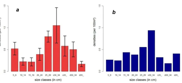
Figure 1: Sparisoma viride phases ... 3 Figure 2: Changes in biomass of Sparisoma viride between 1990 and 1998 ... 5 Figure 3: Size (l) dependent mortality (m) functions: (a) linear: = a*l + , a=-0.02 and b=0.9 (arbitrary) ; (b) exponential: = b*exp a*l , a=-0.2, b=0.9 (arbitrary); ... 8 Figure 4: The growth transition matrix ... 9 Figure 5: Size (TL) at age plots and fitted von Bertalanffy growth equation with estimated Linf and K from non-linear regression of size-at-age data ... 16 Figure 6: logarithmic K and Linf (TL) of Sparisoma viride plot and fitted regression line between logarithmic K and Linf (TL) ... 16 Figure 7: Size distribution of Bonaire (a) and estimated by the model at equilibrium (b), the bars are the densities per size classes represented with the 95%CI for Bonaire

observations ... 18 Figure 8: Mean densities observed in Bonaire per size class with error bars (95%CI) (red dots) and densities per size class estimated by the model (blue crosses) ... 19 Figure 9: Evolution of the model densities (blue) of the 3 habitat categories through time until equilibrium, red lines are the mean densities of Bonaire for each habitat category, the black dot lines delimitate the 95% CI ... 20 Figure 10: Evolution of the model densities of the 3 habitat categories small (S), large shallow (Ls), large deep (Ld), subject to 3 initial conditions (note the scales are different for the 3 plots) ... 21 Figure 11: Size distribution of Bonaire at equilibrium with optimised parameters for a time step of 12 months ... 22 Figure 12: Evolution of the large deep category density (blue) through time for different values of survivorship (s) red lines are the carrying-capacity (mean density of Bonaire for large deep fish), black dots lines are the bounds of the 95%CI ... 23 Figure 13: Evolution of fits (Fval) for different values of r (a) and s (b) ... 24 Figure 14: Evolution of the total density of the parrotfish population after fishing

disturbance ... 24 Figure 15: Size distribution of Sparisoma viride in Belize and Bahamas, bars are the mean densities per size class with associated 95%CI ... 27

ix

List of Tables

Table 1: Matrix of parrotfish densities for one time step per category (columns) and per size class (rows) at a time step t; the densities Si, Lsi, Ldi correspond to the size class i, r is the recruitment ... 7 Table 2: Starting points of the values to optimise and their constrained bounds... 14 Table 3: Results of the non-linear regression of size-at-age data, in SL and in TL ... 15 Table 4: Values of input parameters used for the estimation of the growth transition matrix for a time step of 3 months, mm=millimeters ... 17 Table 5: Values of the objective function (Fval) given by type of survivorship ... 17 Table 6: Estimation of the parameters (survivorship function and r) of the model by the Global Search solver ... 17 Table 7: Mean densities of Bonaire with associated standard errors (SE) and estimated densities by the model at equilibrium for the 3 habitat categories for total density of S. viride ... 19 Table 8: Optimised values of s and r a time step of 12 months and a time step of 3

months standardised to a time step of 12 months ... 21 Table 9: Densities of mean densities of the 4, 5, 6 cm fish for Glover's reef and 3 sites of the Bahamas ... 26

1

Introduction

Coral reefs are well known for being very important marine sources of biodiversity and for supplying many nations with goods and services such as fishing and tourism activities (Hughes, 1994; Hughes et al., 2003). However, in the past decades, the health of coral reefs has been severely degraded, due to a combination of natural events (hurricanes, coral bleaching) and anthropogenic disturbance such as pollution and overfishing (Hughes et al., 2003; Hoegh-Guldberg et al., 2007). It is estimated that nowadays 30% of coral reefs in the world are heavily damaged (Hughes et al., 2003). Coral reefs in the Caribbean have been severely impacted and the situation is critical (Mumby et al., 2006). Because of the multiplying source of disturbances, in many places the reef community structure has shifted from a coral-dominated to a macroalgal-dominated state (Hughes 1994; Hughes et al. 2003). In regards of climate change and ocean acidification, disturbances are expected to rise and worsen the health of Caribbean coral reefs. There is an urgent need to develop local strategies for managing coral reef resilience and biodiversity in the Caribbean.

Herbivory is one of the most important ecological functions driving the resilience of Caribbean reefs. Indeed, herbivores organisms (mostly sea urchins and fish) graze algae growing on the dead coral substrate (Burkepile and Hey, 2008; Mumby and Steneck, 2008) thus liberating space for coral recruits and growth. Without this grazing activity by herbivores, coral life cycle is negatively affected by overgrowing algae and the maintenance a coral-dominated state is impaired (Hughes et al., 2007; Mumby and Steneck, 2008). The sea urchin Diadema antillarium was the main grazer in the Caribbean in the past but between 1983 and 1984, due to a disease, it experienced high death levels (Mumby, 2006; Carpenter, 1990; Lessios, 1988) depriving the Caribbean reefs from its main algal grazer. Since then, Scaridae (parrotfish) became the most important grazer in the Caribbean (Mumby, 2006), representing over 80% of the biomass of herbivorous fishes in the Caribbean (Mumby, 2009).

In the past decades, the number of top-carnivore species, such as snappers and groupers, has dropped to very low levels (Mumby et al., 2007). As a result, parrotfish have become a target species with interesting commercial value for many countries of the Caribbean such as Saba, Puerto Rico, St Lucia, Jamaica and Dominica (Hawkins and Roberts, 2003). However, little is documented on parrotfish landings every year in the Caribbean and no possible stock assessment has been conducted so far (FAO, 2011).The abundance and the biomass of parrotfish are clearly higher in the areas where the fishing pressure is the lowest (Bonaire) compared to high fishing pressure areas (Dominica, Jamaica) (Hawkins and Roberts, 2003; Tuya et al., 2007). In highly fished areas, the size-distribution of exploited parrotfish populations is affected with a decrease of the largest individuals and a global decrease of the average size (Hawkins and Roberts, 2003). Some parrotfish species are hermaphrodite and can change sex during their life, and fishing seems to affect sex-changing: females tend to transform into males at smaller sizes in heavily fished islands (Hawkins and Roberts, 2003).

In many areas parrotfish populations have been depleted due to intense trap fishing (Hawkins and Roberts, 2004). Traps are well known to have very high depletory effects on fish populations (Wolff et al., 1999; Hawkins and Roberts, 2007) but traps are unfortunately one of the most used fishing gear on Caribbean coral reefs (Gobert, 1988). As a consequence, fishing affects the levels of fish herbivory, thus compromising the ability of corals to recover from disturbances (Mumby et al., 2007; Mumby and Steneck, 2008). Therefore, the maintenance of serviceable levels of fish herbivory is now a major concern for the conservation of Caribbean coral reefs. Restoring and protecting parrotfish populations are expected to moderate the future effects of bleaching events rising in frequency and severity with climate change (Mumby et al., 2006; Edwards et al., 2011).

2

Face to global warming and ocean acidification, it is necessary to protect parrotfish species by acting locally with management actions. Protecting parrotfish is sought to delay the negative effects of climate change by maintaining a serviceable level of herbivory for coral reef resilience (Mumby et al., 2013). Yet, implementing efficient management action requires sufficient knowledge on parrotfish population dynamics. But while the importance of parrotfish ecological role is well appreciated, little is known on parrotfish natural mortality, fishing mortality, biomass production, and responses to various fishing pressures. The knowledge on dynamics of the parrotfish is essential to understand the ability to recover from depleted stocks.

Sparisoma viride was chosen for this study for 3 reasons: (1) it is the fish contributing the most to grazing on many Caribbean reefs (Mumby, 2006); (2) S. viride is the most known parrotfish species with available data on it; (3) it is the parrotfish species the most targeted by fishing (Mumby et al., 2006). S. viride is found on the tropical part of Western Atlantic, from Florida to Brazil, including the Gulf of Mexico. The model created in this study is a discrete-time model structured by size and habitat categories (shallow/deep reefs) with the implementation of four ecological processes: natural mortality, growth, recruitment, density dependence in habitat occupation. The model was first calibrated to a time series of fish abundance collected at Bonaire Island, a marine reserve where parrotfish populations are expected to be at equilibrium. In a second step, fishing pressure was added to explore the ability of the model to reproduce the recovery of the parrotfish population. This recovery was compared to the one observed in Bermuda where a fishing ban was implemented.

1. Material and Methods

1.1.

Animal study: Sparisoma viride (S. viride) biology

Parrotfish (family Scaridae, order Perciformes) were named after physical familiarities with parrot birds. Indeed, the assembling of their teeth creates a structure very similar to a parrot’s beak (van Rooij, 1996b) and their feeding mode called “pharyngeal mill”. Parrotfish is a protogynous hermaphrodite; some individuals during their life will experiment sex-changing from female to male to improve their lifetime or increase their reproductive success (Warner, 1987). For parrotfish, sex-changing occurs only one way from female to male, and can be followed by a change in body colour (van Rooij et al., 1996b). Sex-changing is a process requiring a lot of energy but increases the reproductive capacity. Therefore, this is a trade-off between high energetic costs and the number of off-springs potentially produced in the future (Warner, 1987).

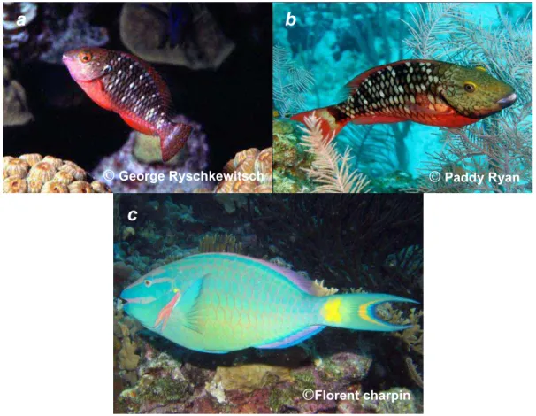
Three different phases can be distinguished in the life cycle of the parrotfish Sparisoma viride (van Rooij et al., 1996b): the juvenile phase (J), the initial phase (IP) and the terminal phase (TP). Juveniles set up on the reef at a length of about 1cm, after a pelagic larval stage (van Rooij and Videler, 1997). After growth and having acquired sexual maturity they become an IP fish. The colour patterns of IP (Figure 1b) fish are close to those of juvenile fish (Figure 1a) (van Rooij et al., 1996b), with a mottled brown colour, white scales and a white vertical band on their tail. TPs colour pattern is significantly different: they are characterized by a blue emerald body and yellow spots on the opercula and at the base of the tail (Figure 1c). IP females can either remain a female for the rest of their life or change sex and colours to become a TP male. However, IP fish can be either male or female (Robertson and Warner 1978; Cardwell 1989). In Bonaire, over 90% of the IP fish are females (van Rooij et al., 1996)). Therefore, they were restricted to females in this study. TP fish are always mature males

3

The particularity of parrotfish population in Bonaire is the spatial and social structure in two different habitats (van Rooij et al., 1996b): a shallow one (<4m) and a deep one (>4m). The deep habitat is divided into social and spatial territories. Each territory is lead by a dominating male the Territorial Terminal Phase male (TTP) and group a harem of 10 to 14 female Territorial Initial Phase (TIP). The number of territories in Bonaire was estimated to 17 with a size range of 240 to 820m². TTPs seemed to show a defending behaviour towards conspecifics with males that do not belong to their territories. This support the assumption that territories are set up mating purposes (van Rooij et al., 1996a).Territorial fish (TTP+TIP) represent less than 20% of the whole population but control up to 77% of the reef (van Rooij et al., 1996b). Every TTP reproduces with its harem every day but also occasionally with non-territorial/group females from the shallow habitat that invade the deep habitat. The shallow habitat has no particular social structure and it groups non-territorial fish, briefly called group fish or shallow fish. This shallow habitat groups females, Group Initial Phase (GIP) and males, Group Terminal Phase (GTP). The Shallow habitat can group up to 14 males and 28 females (van Rooij et al., 1996b). It was observed that GTPs hardly ever reproduce. Their reproducing rate was considered null. The territorial fish are globally bigger than the non-territorial fish: TTPs measure 30-37 cm fork length (FL) and TIP 20-35cm whereas GTP measure 21-39cm FL and GIPs 17-29cm FL. Morphologically, GTPs and TTPs just as GIP and TIPs cannot be distinguished by their colour pattern as it is the same (described above). Unlike mature males and females, juveniles do not belong to a territory or not even to the shallow group. They are equality distributed on the reef.

Figure 1: Sparisoma viride phases: (a) Juvenile phase (flower Garden Banks, Texas, USA),

(b) Initial phase (Glover’s reef, Belize, (c) Terminal phase (Bonaire, Netherlands)

a

b

c

©

George Ryschkewitsch

_©

Paddy Ryan

4

1.2.

Available data on Sparisoma viride

1.2.1. Bonaire time series of abundance data

Bonaire was set up as an entire marine reserve in 1979, well before van Rooij (1996)

parrotfish surveys. The total densities of S. viride as well as the size distribution of the population are considered constant over the period 1989-1992 (van Rooij and Videler, 1997), suggesting a population at ecological equilibrium. Therefore we used this time series to calibrate the model at equilibrium.

van Rooij (1996b) has collected abundance data of S. viride between 1989 and 1992 in Bonaire (Netherland Antilles). Stationary visual censures (Bohnsack and Bannerot 1986)

were performed on quadrats to record fish densities of different phases (J, IP and TP) per 5cm (FL) size class. A number of five permanent quadrats were used to record these densities. Fish quadrats were positioned at increasing depth strata: 0-2m, 2-4m, 4-6m, (10x15m quadrats for the 0-2m, 2-4m, 4-6m ranges and 15x15m for the range quadrats 6-12m and >6-12m). Although no distinction was made between group and territorial TP fish during the survey, this can be inferred by the depth of the quadrates. We classified quadrats as “shallow” (<4m) or “deep” (>4m) habitats according to van Rooij (1996b). The shallow habitat gathers group TPs exclusively, whereas the deep habitat is characterised by the presence of group and territorial TPs, the formers making brief incursions into the deep territories. van Rooij (1996b) thus estimated that approximately 50% of the TP fish surveyed were actually transient group TPs coming from the shallow reef. A number of twenty-six field surveys were performed between 1989 and 1992 and grouped per trimesters. As a result, seven density estimates of S. viride are available in Bonaire for this study.

1.2.2. Growth data Size-at-age data

We used size (in fork length, FL) at age measurements performed on S. viride individuals by Choat et al. (2003) in Los Roques Archipelago (Venezuela). Those data, communicated by Prof. John Howard Choat (School of Marine Biology and Aquaculture, James Cook University, Townsville, Australia), were estimated after otolith processing (Choat et al., 2003). They were used to estimate growth parameters of S. viride population from Los Roques which are assumed to be similar to Bonaire parrotfish populations, since the two reef areas are characterised by a very low fishing pressure and are only distant from 150 km within the same latitudinal range (12° 20’ N).

Information about the growth of S. viride populations in the Caribbean was completed with Fishbase data that was used to calculate growth. Five couples of von Bertalanffy parameters, Linf and K, for S. viride are available on fishbase, mostly from Choat et al., (2003) estimations.

Conversion between parrotfish recorded lengths

Fish sizes having been measured as fork length (FL) in Los Roques, we used available coefficients of conversion between the standard length (SL), fork length (FL) and total length (TL) of S.viride. These conversions are the following:

= . �

�ℎ

. ,

� = .

� ℎ

,

5

1.2.3. Additional data

Bahamas and Belize abundance data

The data recorded in the Bahamas and in Belize were used to compare recruitment and the size distribution of parrotfish population estimated by the model. These data were communicated by Dr. Alastair Harborne (Marine Spatial Ecology Lab, University of Queensland, Australia). The dataset contains the abundance of individuals of S. viride recorded by visual censures along transects. The abundances are given in densities per 120m² and per 1cm size (TL). The surveys were performed on four different sites of the Bahamas (Andros, Exuma Cays Land and Sea Park and San Salvador), in Turk and Caicos island and Glover’s atoll in Belize.

Bermuda abundance data

Abundance data of S. Viride recorded in Bermuda were used to simulate a recovery of the parrotfish population in Bonaire after a virtual fishing disturbance. In Bermuda, a fishing ban was decided in April 1990 (Luckhurst, 1999) due to a high decrease of many reef fish (Butler

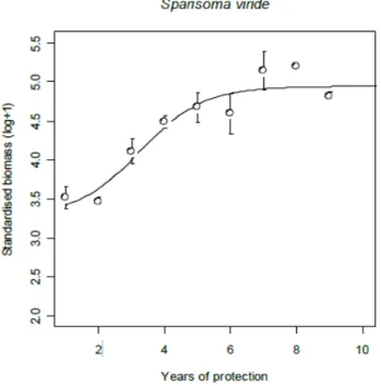
et al., 1993). However, only trap fishing was completely banned and hook-a-line fishing targeting top predators essentially was still authorized. After the implementation of the fishing ban, S. viride populations were monitored at regular time intervals using stationary visual censuses (Luckhurst 1999). A first analysis of this dataset (O’Farrell, 2011) has shown that parrotfish populations recovered and reached a maximum in only 8 years (Figure 2). The abundance of parrotfish population was multiplied by 2-3 during this 8 years period (O’Farrell, 2011).

Figure 2: Changes in biomass of Sparisoma viride between 1990 and 1998 (from O’Farrell, 2011)

biomass is given is relative abundance to the first observation

1.3.

Model development

1.3.1. Choice of the type of model

6

to reproduce observations of parrotfish recovery in Bermuda after the ban on fish traps in April 1990. This model was empirical and its ability to describe population size structure was limited to 3 broad size classes. Moreover, transitions between classes incorporated mortality but without being clearly explicit. Therefore, a more mechanistic model, structured by size with the incorporation of an explicit natural mortality and growth was developed in this study. The present model also includes recruitment and density dependence. The density dependence is assumed to be reflecting the saturation of TP territories in the deep habitat, which limits the emigration of new fish from shallow reefs.

The model was developed using Matlab for several practical reasons: 1) Matlab is an appropriate modelling software for matrix calculation; 2) Matlab has a very performing optimisation program (Optimisation Toolbox) to estimate the parameters of the model; 3) the model will be integrated in fine in a model of coral reef ecosystem, ReefMod (Mumby et

al., 2006; Edwards et al., 2011), which describes the competition between corals and algae under the influence of herbivory, and which is currently developed in MatLab language.

1.3.2. Model structure

The model is structured by size and habitat categories. It recreates the evolution through time of the parrotfish densities.

Time step of the model

A time step of 3 months was chosen for the model regarding the observations in time of Bonaire data. However, this time step is easily adaptable to other datasets studies and only needs to be changed only once in the script.

Structure by Size classes

The model was designed in size classes because it aims at becoming a useful tool for fisheries management. With a structure in size classes, there is the possibility to predict the effect of fishing on parrotfish size distribution when simulating different fishing scenarios. Size classes were designed from Smin TL to Lmax TL in centimeters with an increment of 1 cm. Smin is the minimum size of fish considered in the model and Lmax is the maximum one. The model is designed in TL unlike Bonaire data recorded in FL because this study aims at becoming a useful tool for fisheries management. We defined Smin=5cm and Lmax=Linf. The recorded densities of fish below 5cm are usually underestimated when surveyed (Bozec et al., 2011), we ignore the early stage processes occurring for the smallest fish. Therefore, sizes below 5cm TL were ignored in the model. Linf is the maximum hypothetical size of S. viride from von Bertalanffy equation. The calculation method of Linf is explained in 1.3.3.

Structure by habitat categories

The purpose of a division of fish into two habitats categories (shallow and deep reef) is to reproduce the particular spatial and social structure of the parrotfish population observed in Bonaire. The model reproduces the migration of shallow fish to the deep habitat. Indeed, in Bonaire, males can migrate when taking over a territory and female when becoming part of a TTP harem in a territory. We defined 3 habitat categories for S. viride: (1) shallow+deep for small (J+IP+TP) fish (<30 cm FL), (2) shallow for large (adult IP+TP) fish (>=30cm FL), (3) deep for large (adult IP+TP) fish (>=30cm FL). Only TPs above 30 cm FL were observed in the territories (van Rooij et al., 1996b). The small fish do not belong to a particular habitat and are assumed to be equally distributed on the reef. The migrations are implemented in the model by a transition of large shallow fish to large deep category. As their name indicates, the large shallow fish are constrained to the shallow habitat and the large deep fish to the deep habitat. The small fish bounds are Smin and Smax where Smax is the

7

maximum size of the small fish. The large shallow and large deep bounds are Lmin and Lmax where Lmin is the minimum size of large fish. Smin and Lmax are defined as above. The Large fish category bounds were defined regarding the size distribution of the TTPs in Bonaire: 62% of the TTPs belong to the 30-35 cm FL class and 38% to the >40 cm FL class. Therefore in the case of this study, Lmin=30cm FL. Smax is an increement lower than Lmin therefore, Smax=29cm FL. However, IP of the deep habitat in Bonaire measure 20-35cm FL and IP of the shallow measure 17-29cm FL. The number of IPs in the large deep category is then slightly underestimated and overestimated in the large shallow category, but the correct number of TTPs is properly estimated. If Lmin was equal to 20cm FL like TIP size range suggested, the density of TTP fish and more generally the density of fish in the deep habitat, would have been overestimated. The large deep fish would have represented over the 20% of the population they actually represent in Bonaire.

A representation of the model structure for one time step is given in Table 1. There is no overlap between Small and Large fish: Small fish are strictly restricted to the size range Smin to Smax. Therefore, the densities of the small fish from Lmin to Lmax are always equal to zero. Large shallow and Large deep fish are restricted to the same size range Lmin to Lmax. Therefore the densities from Smin to Smax of both large shallow and large deep are always null (Table 1).

Table 1: Matrix of parrotfish densities for one time step per category (columns) and per size class

(rows) at a time step t; the densities Si, Lsi, Ldi correspond to the size class i, r is the recruitment

Habitat Categories Sizes(in cm, TL)

SMALL LARGE SHALLOW LARGE DEEP

Smin=5 r 0 0 6 0 0 0 7 0 0 0 ... S6 0 0 31 ... ... ... Smax=32 S32 0 0 Lmin=33 0 Ls33 Ld33 … ... … …

Lmax=Linf 0 LsLinf LdLinf

1.3.3. Model parameterisation

In the model, within a time step of 3 months the parrotfish population experiences 4 ecological processes: natural mortality, growth, recruitment and density dependence.

Natural mortality

Only natural mortality was implemented in the model. No fishing mortality was considered in the first part of the study. To implement natural mortality in the model, two options were possible: implementing a constant mortality rate per size or implementing a size dependant mortality function. The mortality parameter stands for all the different types of natural mortality: mortality per predation, per senescence, per sickness and any factor inducing natural mortality other than by fishing.

Constant instantenous rate of natural mortality per size

8

data collected at Los Roques Archipelago in Venezuela. To calculate this instantaneous mortality rate, Choat et al. (2003) used a linear regression of the logarithm of the age-frequency and the age at size. The regression slope gives the mortality per year (more details in Choat et al., 2003). At Los Roques, the mortality was estimated to be: = . . The associated survivorship per year using the exponential conversion is = − _{= . . In} the model, the survivorship was used instead of the mortality for more convenience. This survivorship s was converted for a time step of 3 months by the following operation:

= . _ �/ _{, _ = , = .}

At each time step of 3 months, this constant rate of survivorship per size was multiplied by the density of each size class which means that 94% of the population survives at each time step.

Size dependent mortality

 Linear size dependent mortality

Because smaller sizes are more vulnerable to predation and then assumed to have a higher mortality compared to larger fish, we tested a size dependant mortality relation. First by implementing a simple linear relation: = a*l + , where is the mortality, l is the length in TL of the fish, a and b are respectively the slope and the intercept of the mortality line. This mortality relation is based on the assumption that mortality is decreasing (a< ) linearly with the size of the fish (Figure 3a). b is the hypothetical mortality rate that would have a fish of size 0cm. The associated survivorship is = − .

 Exponential size dependent mortality

A more complex size-dependent mortality function was: = b*exp a*l , where is the mortality, l is the TL of the fish, a and b are respectively the slope and the intercept of the mortality curve. As previously, this mortality function is based on the assumption that mortality decreases when the size of the fish increases. In this case, compared to a linear mortality, there is the existence of a threshold: from a certain size, 25cm (Figure 3b), and a fish can escape mortality per predation which appears more realistic. The associated survivorship is = − .

Figure 3: Size (l) dependent mortality ( ) functions: (a) linear: = a*l + , a=-0.02 and b=0.9 (arbitrary) ; (b) exponential: = b*exp a*l, a=-0.2, b=0.9 (arbitrary);

In our study, we used the survivorship s instead of the mortality for practical reasons in the implementation. However, we named a and b the respective slope and intercept of the size-dependant mortality functions.

9

Growth

To implement growth in the model, we used a growth transition matrix because the model is structured by size. Therefore, this matrix was necessary to implement growth transitions between size classes. Growth transition matrices give the probabilities of growing from one size class into others within a given time step. An example of growth transition matrix is given in Haddon (2011) (Figure 4). In Haddon (2011) the growth matrix is calculated using a probability density function. However, the growth matrix of Haddon required parameters we were unable to obtain with our data. We decided to use the growth transition matrix developed by Chen et al. (2003). The construction of this matrix is based on the same assumptions than Haddon (2011). However, Chen et al. (2003) growth matrix is more precise because its calculation takes in consideration the difference of growth rates between smaller fish and larger fish. Smaller fish grow faster than larger fish during the same period of time. Moreover, Chen et al. (2003) growth matrix required inputs that could be calculated with data we obtained from Pr. J. Choat. This growth transition matrix is generated by the function growtrans from the R package Fishmethods created by Chen et

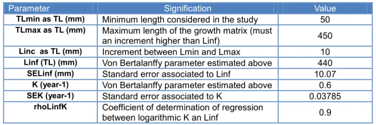
al. (2003). For each size class, growtrans calculates the probabilities to grow from a size to others within a year using the von Bertalanffy equation. Eight inputs are needed for the calculation of this matrix: TLmin, TLmax, Linc, Linf and K (parameters of the von Bertalanffy equation) and their associated standard errors SELinf and SEK, and finally the coefficient of determination between Linf and K, rhoLinfK, obtained from a regression between ln(K) and ln(Linf). Using these 8 inputs and von Bertalanffy equation, the growtrans function realises Monte Carlo simulations to generate probabilities for a fish of a particular size to grow to another length within a time step. In our model, this matrix is constant through time and is calculated before model simulations. Any change in the time step requires a recalculation of this growth matrix with the appropriate time step.

Figure 4: The growth transition matrix: Gi,j are the probability that one fish of size class j will grow in size classes i at the considered time step (from Haddon, 2011, chapter 13, Figure 13.2)

 Defining TLmin, TLmax, Linc

TLmin, TLmax and Linc are defined in millimeter. TLmin was set up at 50 mm like the starting length of the model, Lmax=Linf+1 as Lmax must be an increment higher than Linf (Chen et al. , 2003). Like in the model, the increment was chosen equal to 1cm, Linc=10mm.

 Calculation of Linf and K and their associated standard error

To calculate Linf and K and their associated standard errors Choat et al. (2003) data of size-at-age were used. These size-size-at-age data were fitted the von Bertalanffy equation:

= − − −0 )

Where Lt is the estimated size of a fish at age t, Linf and K are the parameters of the equation

of von Bertalanffy, and t0 is the estimated age at the hypothetical size 0. We used in our

study the t0=0.06 estimated by Choat et al. (2003) for the S. viride population of Los Roques.

10

(Ritz and Streibig, 2009).This regression was processed after conversion of FL data in TL as the model is structured in TL. We also performed this regression in SL to compare our results with the results obtained in SL by Choat, et al. (2003).

 Calculation of rhoLinfK

To calculate the coefficient of determination between Linf and K, we used the 5 couples of Linf and K of S. Viride available in fishbase data. We applied the method developed in Chen

et al. (2003). This method is based on the assumption that Linf and K are negatively correlated: populations or species whose Linf is high, tend to have a lower K, and vice versa (Chen et al., 2003). This calculation method consists in doing a linear regression between ln(K) and ln(Linf). The coefficient of determination of this regression is the input of the growth transition matrix.

Recruitment

In this study, we defined recruitment as a constant addition of 5cm fish in the population at each time step. In the model, a recruit is a juvenile fish of 5 cm settled on the reef that already experienced mortalities due to the early stages. This size threshold (5 cm) in the definition of recruits was chosen since no information is available these early stages. In addition, no abundance data of fish less than 5cm can be reliably used due to biases in surveys (Bozec et al., 2011). The model also ignores any stock-recruitment relationship.

Density dependence in the deep habitat

As observed by van Rooij andVideler (1997), the number of territories in the deep habitat is limited. Consequently, the density of fish in the deep habitat is limited. The maximum density of the deep habitat is the carrying-capacity ( _Ld). When a TTP leaves its territory (through migration or mortality), a GTP replaces it. IP females can also migrate from the shallows to become part of one TTP’s harem. These migrations of the fish from the shallow to the deep were reproduced in the model by implementing a transition rate. The transition matrix _Ls→Ld from Ls to Ld gives the proportion of Ls transiting to Ld, this proportion is weighted by the density of each size class in the Ls category by Lsl,t

∑Lsl,t., where ∑Lsl,t is the

total density of Ls of all sizes at time step t. The transition proportion of Ls transiting varies at every time step and is estimated based on the carrying capacity _Ld of large deep population by ∑Ldl,t

Ld , where ∑Ldl,t is the sum of the Ld of all sizes.

The transition matrix from Ls to Ld is given by:

Ls→Ld= ( −∑Ldl,t

Ld )

Lsl,t ∑Lsl,t

1.3.4. Model implementation and outputs

Model implementation

 Habitat categories

There is no overlap between categories S, Ls and Ld. If after experiencing growth, a small fish becomes larger than Smax, it automatically transits to the Ls category. Small and large shallow categories could have been grouped together in one single category from Smin to Lmax. However, they were distinguished in 2 categories. First because large shallow fish represent fish constrained to the shallow habitat whereas small fish are equally distributed on the entire reef with no habitat distinction. Secondly, separating small and large shallow allowed us to implement and represent density dependence in the deep habitat more easily.

11

 Recruitment

The addition of 5cm fish is made after all other processes described above.  Density dependence

Only large shallow fish are given the possibility to transit to the large deep category if the carrying capacity of the deep fish was not reached at the previous time step. Small fish cannot transit directly to the large deep fish (van Rooij et al., 1996c). However, if after growth, a small fish transited to the large shallow category, it is then eligible to transit to the large deep category within the same time step.

 A flexible model

The model was created to be first calibrated with Bonaire data. Consequently, the categories, size classes, and the parameters were implemented following Bonaire observations. However, the model is very flexible and adaptable and the time step can be easily changed, as well as the size limits Smin/Smax and Lmin/Lmax. In addition, the model is designed in TL but the model outputs can be converted in FL or SL given the empirical relationships presented above. The recruitment and the carrying capacity of large deep fish can also be changed in the model. The structure in habitat categories can also be removed to keep a structure in size classes only. Only the growth transition matrix would need to be recalculated if using another Linf and K, and time step. The structure of this model was then made to be as general and flexible as possible because this study aims at being generalized at other parrotfish species and other sites of the Caribbean.

The model

��, +� = ( ��, )( − �→ �) +

� �, +�= � �, + ��, �→ � − →

���, +�= ���, + � �, + ��, �→ � →

, + , , + , , + are respectively the densities of the small, large shallow and large deep categories at time t+1 and size l

, , , , , are respectively the densities of the small, large shallow and large deep categories at time t and size l

is the size-dependent survivorship

gl is the growth probabilities for a fish of size l r is the recruitment

�→� the transition matrix from S to Ls. It includes the matrix of 0 and 1 values to control the transition

of S fish of appropriate size (every fish larger than Smax automatically switches from S to Ls) �→� is the transition matrix from Ls to Ld. It gives the proportion of Ls transiting to Ld, those

proportions varies at every time step and are estimated based on the carrying capacity of Ld population

Outputs of the model

As the purpose of the study is recreating the size distribution observed in Bonaire with the model, we represented the densities per size classes as outputs of the model. These size classes are the following (in FL): 5-9cm, 10-14cm, 15-19cm, 20-24cm, 25-29cm, shallow 30-34cm (s30-34cm), shallow>35cm(s>35cm), deep 30-34cm(d30-34cm), deep>35cm

12

(d>35cm). We summed the densities of the size classes of the model having an incremement of 1cm to obtain these output size classes. We grouped together for each habitat the size classes 35-39cm and >40cm. First, because the density of fish over 40cm is very low therefore the >40cm fish did not need a particular size class. Secondly, with a time step of 3 months, fish from 35cm and above remain at each time step at their current length and do not grow enough. Therefore, in terms of growth, there is no possibility to distinguish a fish from the size class 35-39cm and the size class >40cm.

1.4.

Model calibration: population at equilibrium

1.4.1. Re-organisation of Bonaire data

Re-organisation of the categories and size classes

The model was first calibrated with Bonaire data as the population of S. viride is considered at equilibrium. For this purpose, Bonaire data were reorganised because the model is not structured life phases (does not involve sex change transition) like these data. In addition, this new organisation was necessary in order to implement density dependence occurring in the deep reef of Bonaire. These size classes are the same described in the output of the model. We also reorganised the data in habitat categories like in the model: in the data, the small fish category was created by summing the J, IPs and TPs of size range 5-29cm FL. Large shallow and large deep categories were created by summing the IPs and TPs from 30-34cm to >40cm of the corresponding habitat (shallow or deep).

 Re-organisation in categories: Small, Large shallow and Large deep fish

Large shallow fish groups together all the fish of size range 30cm-40cm FL, of the shallow quadrats (<4m), independently from their life phase (IP+TPs).

Large deep fish groups together all the fish of size range 30cm-40cm FL, of the deep quadrats (>4m), independently from their life phase (IP+TPs).

Small fish are the fish covering the size range 1-29cm FL independently from their life phase (J+IP+TPs). Small fish are assumed to be equally distributed on the reef (van Rooij and Videler, 1997). Therefore, we organized the Small fish independently from the depth they have been recorded. The densities of TTPs and GTPS had to be adjusted in the data. Indeed, the invasion by GTP of TTPs territories conducted to overestimate the number of TTPs (van Rooij and Videler, 1997). Therefore, the density of TPs in the deep quadrats (standing for TTPs) was halved and the other half was added to TPs of the shallow quadrats standing for GTPs (van Rooij and Videler, 1997). To estimate the mean density per category, we aggregated the data per observation and per type of habitat and proceeded to the adjustment of TPs following van Rooij procedure. We then calculated the mean density for each category (S, Ls, Ld) on Bonaire times series and associated standar errors.

 Re-organisation in size-classes

The re-orginisation of Bonaire data follows the same scheme as the output of the model to ease comparison. To create the small fish size classes (from 5-9cm to 25-29cm FL) from Bonaire, we summed for each observation, the fish (J+IP+TP) densities corresponding to the range of the size class. Then, we calculated the mean and associated standard error of theses size classes over the time series of Bonaire. For the Large fish size classes (30-34cm and >35cm FL), we summed the fish (IPs+TPs) densities of the shallow quadrats for the large shallow fish and of the deep quadrats for the large deep fish. We calculated the mean and associated standard error for each habitat category.

Implementing initial conditions in the model

Densities per size classes in Bonaire were used as initial conditions for the model. However, Bonaire size classes have an increment of 5cm and the model have an increment of 1cm

13

for the size classes. Therefore, the density of each observed size class converted in TL was divided by five in order to determine the initial density of the 1-cm size classes of the model.

1.4.2. Optimisation of model parameters

We optimised two parameters of the model: natural mortality and level of recruitment (density of fish entering the model at 5cm). Using optimisation we also tested the 3 different formulations of natural mortality on model fits to Bonaire data.

Optimisation method with the Global Search solver

The Global Search solver from Matlab optimisation toolbox was used to optimise the parameters of this study. Global Search is designed to find one global minimum and other local minima of an objective function, using a constrained nonlinear optimisation solver. We used fmincon as the constrained nonlinear solver. The solver fmincon is designed to find a local minimum around a starting point. Global Search set up multiple starting points using a scatter-search algorithm (Mathworks, Global Optimisation Toolbox, 2013). Then, it filters non-promising starting points based upon objective and constraint function values and local minima already found. Finally, Global Search runs fmincon from the remaining starting points to find minima around these starting points. Among all the local minima found, the one considered as the global minimum of the objective function is the one having the lowest value of this objective function (Mathworks, Global Optimisation Toolbox, 2013).

Application of the optimisation method

In this study, the objective function to minimise with the Global Search solver is the sum of squared differences between the model estimations and Bonaire observations for of the 9 size classes described previously. The optimisation aims at reproducing the size distribution observed in Bonaire with the model by minimising the sum of squared differences. The optimisation is based on a confrontation between densities per size classes estimated by the model and mean densities per size classes observed in Bonaire. We chose not to optimise using the habitat categories as they have only been designed to implement the density dependence parameter. With this method, we tested the 3 functions of survivorship described previously: (1) we tested the constant rate of survivorship and the associated value of recruitment r by optimising theses 2 values, (2) we tested each of the 2 size dependant survivorship functions by optimising the slope a and the intercept b of the mortality functions, and the associated value of recruitment r.

Starting points and bounds

For each of the value to optimise, s, a, b and r, initial values and bounds are required for Global Search to work. In addition, they must have ecologically meaningful values. As r is a totally arbitrary value, a wide range of values was given (Table 2). s is a survival rate, therefore s can only vary between 0 and 1. For the parameters a and b of the size dependent mortality functions, we chose the same values: a (slope) must be negative as we assume that mortality decreases with the size and b (intercept) is assumed to be constrained between 0 and 1 as it represents the mortality of a fish of hypothetical size 0. For starting points, after adjusting the model by hand, we chose the values that seemed to provide the best fit to the data.

14

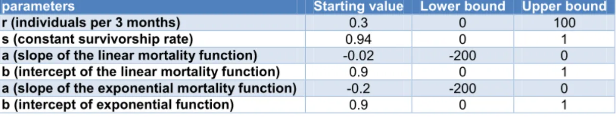
Table 2: Starting points of the values to optimise and their constrained bounds

parameters Starting value Lower bound Upper bound

r (individuals per 3 months) 0.3 0 100

s (constant survivorship rate) 0.94 0 1

a (slope of the linear mortality function) -0.02 -200 0

b (intercept of the linear mortality function) 0.9 0 1

a (slope of the exponential mortality function) -0.2 -200 0

b (intercept of exponential function) 0.9 0 1

1.4.3. Exploration of the optimised model

The model behaviour was explored with the optimised parameters. This step is required to understand the impact of these parameters on the model at equilibrium.

Influence of the initial conditions

We tested the evolution of the densities of the 3 habitat categories when implementing different initial conditions. Three sets of initial conditions were tested are: (1) the initial conditions of Bonaire, where the 9 initial densities correspond to the average densities observed in Bonaire between 1989 and 1992, (2) initial conditions set arbitrary to lower densities than Bonaire from 1989 to 1992 (all densities equal to 0); (3) initial conditions set arbitrary to higher densities than Bonaire from 1989 to 1992 (all densities equal to 1). Influence of the time step

We tested the influence of a different time step (12 months) on the size distribution estimated by the model at equilibrium. A new growth transition matrix was calculated accordingly, and model parameters were optimised in a similar manner to the 3-month time step model. Size distributions of both models were assessed visually.

Influence of the survivorship s on the density dependence

We tested the influence of different values of the survivorship on the large deep category density and its ability to reach its carrying capacity.

1.4.4. Sensitivity analysis of the model to the parameters

We tested the sensitivity of the model to survivorship s and recruitment r. We used a method consisting in fixing one of these two parameters at the optimised value and making the other parameter vary within a defined range of values. The effects of these variations were observed on the variations of a fit. For this fit, we used the objective function described in the optimisation method.

r (recruitment) was made to vary between + and – 30% of its optimised value with a 10% increment

s (survivorship) was made to vary down to -30% of its optimised value with a 10% increment. For higher values, only two values 0.94 (Choat et al. (2003) survivorship) and 0.98 were chosen. Indeed, s cannot exceed 1.

1.5.

Model application: recovery after applying fishing pressure

The model was used for a preliminary approach of calibration to the data collected in Bermuda. In Bermuda, after the implementation of a fishing ban (on traps only), the S. viride population recovered in 8 years only. A plateau was reached after 8 years and the recovery factor was 2-3. With the model calibrated on Bonaire data, we simulated fishing disturbance equivalent to the one in Bermuda before the fishing ban: we divided the densities of the size

15

classes by the recovery factor in Bermuda. Then, we ran the model to test if the speed of recovery was similar to the one observed in Bermuda.

2. Results

2.1.

Model construction: the Growth Transition Matrix

Non-linear regression of size-at-age data

Choat et al. (2003) data were used to estimate Linf and K and their associated standard errors that are necessary inputs for the estimation of the growth transition matrix (Chen et

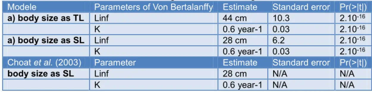
al., 2003). We re-estimated Linf, K by performing a non-linear regression between sizes and ages of S.viride individuals following the von Bertalanffy equation. The results are given for the regressions with body size expressed as TL and SL (Table 3).

Table 3: _{Results of the non-linear regression of size-at-age data, in SL and in TL}

Modele Parameters of Von Bertalanffy Estimate Standard error Pr(>|t|)

a) body size as TL Linf 44 cm 10.3 2.10-16

K 0.6 year-1 0.03 2.10-16

a) body size as SL Linf 28 cm 6.2 2.10-16

K 0.6 year-1 0.03 2.10-16

Choat et al. (2003) Parameter Estimate Standard error Pr(>|t|)

body size as SL Linf 28 cm N/A N/A

K 0.6 year-1 N/A N/A

Because sizes in our population model are expressed in TL, Linf in TL was used to estimate the growth transition matrix. Figure 5 represent the sizes (TL) at age plots with the fit of the von Bertalanffy growth model.

16

Figure 5: Size (TL) at age plots and fitted von Bertalanffy growth equation with estimated Linf and

K from non-linear regression of size-at-age data

Correlation between logarithmic K and Linf

The linear regression between logarithmic K and Linf values provided by Fishbase was performed with the R lm function. The adjusted coefficient of determination (R²) of this relationship is 0.90 (Figure 6). These estimates was subsequently used as an input for the calculation of the growth transition matrix (Chen et al., 2003).

Figure 6: Logarithmic K and Linf (TL) of Sparisoma viride plot and fitted regression line between logarithmic K and Linf (TL), ln = . − . ln , � =0.008534, . ² = . ,