HAL Id: inria-00520606
https://hal.inria.fr/inria-00520606
Submitted on 20 Mar 2012
HAL is a multi-disciplinary open access
archive for the deposit and dissemination of
sci-entific research documents, whether they are
pub-lished or not. The documents may come from
teaching and research institutions in France or
abroad, or from public or private research centers.
L’archive ouverte pluridisciplinaire HAL, est
destinée au dépôt et à la diffusion de documents
scientifiques de niveau recherche, publiés ou non,
émanant des établissements d’enseignement et de
recherche français ou étrangers, des laboratoires
publics ou privés.
Hereditary Substitutions for Simple Types, Formalized
Chantal Keller, Thorsten Altenkirch
To cite this version:
Chantal Keller, Thorsten Altenkirch. Hereditary Substitutions for Simple Types, Formalized. MSFP
-Third Workshop on Mathematically Structured Functional Programming - 2010, Sep 2010, Baltimore,
United States. �inria-00520606�
Hereditary Substitutions for Simple Types, Formalized
Chantal Keller
∗ INRIA Saclay–Île-de-France France ❦❡❧❧❡r❅❧✐①✳♣♦❧②t❡❝❤♥✐q✉❡✳❢rThorsten Altenkirch
The University of Nottingham United Kingdom t①❛❅❝s✳♥♦tt✳❛❝✳✉❦
Abstract
We analyze a normalization function for the simply typed λ-calculus based on hereditary substitutions, a technique developed by Pfenning et al. The normalizer is implemented in❆❣❞❛, a total language where all programs terminate. It requires no termina-tion proof since it is structurally recursive which is recognized by ❆❣❞❛’s termination checker. Using ❆❣❞❛ as an interactive theo-rem prover we establish that our normalization function precisely identifies equivalent terms and hence can be used to decide βη-equality. An interesting feature of this approach is that it is clear from the construction that βη-equality is primitive recursive. Keywords Hereditary substitutions, Type Theory, normalizer, de-cidability of βη-equality
1.
Introduction
Among the different ways to establish the decidability of some equality for λ-calculi (e.g. see [6, 16]), it seems natural in a pro-gramming point of view to give a normalization function, and to prove that it computes a canonical form for any term. This approach is well-suited for an implementation, and it thus becomes important to be able to analyze it in order to prove, for instance, termination of the process.
In this paper, we define a normalizer that β-reduces and η-expands simply typed λ-terms. We use it to establish a formal verification of the decidability of the βη-equality for this calculus.
The normalizer and the proofs are implemented in❆❣❞❛ [1, 13]. ❆❣❞❛ is a programming language with dependent types. We ex-ploit this property in two ways. First, the typing system is powerful enough to ensure some non trivial properties of the functions de-fined in this language. Secondly, we can use❆❣❞❛ as an interactive theorem prover.
Thus,❆❣❞❛ is our metalanguage all along the paper. The source code can be found online [2].
This paper explains our implementation choices and gives the main ideas of the proof of decidability of the βη-equality.
We consider a typed syntax for λ-calculus, that is to say we con-sider only well-typed terms (Section 2). It uses De Bruijn indices,
∗Secondary affiliation: École Normale Supérieure de Lyon, France
which are adapted to a formal development since closed terms have a unique form (Section 2.2).
The normalizer implements hereditary substitutions (Section 3) [17], which preserve canonical forms by substituting and reducing the redices that can appear from substitution at the same time. An important aspect of hereditary substitution is that it can be defined using structural induction; hence, it can be implemented in total Type Theory without any termination proof. In our development, ❆❣❞❛’s termination checker is able to check that the normalizer does terminate (Section 3.4).
We prove the completeness (Section 4) and the soundness (Sec-tion 5) of our normalizer, in order to conclude that it decides the βη-equivalence of two terms.
We finally discuss related work (Section 6) and conclude (Sec-tion 7).
2.
The simply typed λ-calculus
We start by introducing our calculus. Its particularity is that we only define well typed terms: terms are objects of an inductive family parameterized by types. This presentation of the simply typed λ-calculus is formally described in [7], for instance. It is very convenient to use in❆❣❞❛, which supports dependent type programming and inductive declarations.
2.1 The calculus
The set of types (❚②) is defined by a simple inductive definition: ❞❛t❛ ❚② : ❙❡t ✇❤❡r❡
◦ : ❚②
❴⇒❴ : ❚② → ❚② → ❚②
Inductive definitions are introduced in❆❣❞❛ with the keywords ❞❛t❛ and ✇❤❡r❡. Each following line defines a new constructor of this inductive type, giving its type.❙❡t is ❆❣❞❛’s type of types, and the❴•❴ notation is used to define mixfix operators.
For terms, we use (typed) De Bruijn indices to represent vari-ables [11]. We thus need a context that maps each free variable to a type. Since we do not have to store names, a context (❈♦♥) can be represented as a list of types:
❞❛t❛ ❈♦♥ : ❙❡t ✇❤❡r❡ ε : ❈♦♥
, : ❈♦♥ → ❚② → ❈♦♥
As explained above, the sets of variables (❱❛r) and terms (❚♠) are objects of an inductive family indexed by types and contexts:
❞❛t❛ ❱❛r : ❈♦♥ → ❚② → ❙❡t ✇❤❡r❡ ✈③ : ❢♦r❛❧❧ {Γ σ} → ❱❛r (Γ, σ) σ
✈s : ❢♦r❛❧❧ {τ Γ σ} → ❱❛r Γ σ → ❱❛r (Γ, τ) σ ❞❛t❛ ❚♠ : ❈♦♥ → ❚② → ❙❡t ✇❤❡r❡
Λ : ❢♦r❛❧❧ {Γ σ τ } → ❚♠ (Γ, σ) τ → ❚♠ Γ (σ ⇒ τ) ❛♣♣ : ❢♦r❛❧❧ {Γ σ τ } →
❚♠ Γ (σ ⇒ τ) → ❚♠ Γ σ → ❚♠ Γ τ
In❆❣❞❛, curly brackets surround the implicit arguments of a constructor or a function. Usually, these arguments can be auto-matically infered by❆❣❞❛, so they do not have to be given when the constructor or the function is applied. For a matter of space, in the paper, we skip them also in type declarations when it does not lead to any ambiguity: we consider that any symbol appearing in the type of a constructor or a function that is not previously defined is an implicit argument. For instance, the type of❛♣♣ would now be written:
❛♣♣ : ❚♠ Γ (σ ⇒ τ) → ❚♠ Γ σ → ❚♠ Γ τ 2.2 Working with De Bruijn indices
De Bruijn indices have the nice property to give a unique represen-tation to any closed term, which makes them easy to implement. They are not natural to use for a human being, though. For clarity, this section presents some tools to work with De Bruijn indices in our calculus.
2.2.1 Vocabulary
First, we use a rigid vocabulary all along the paper: •If①✿ ❱❛r Γ σ, we call ① an index.
•If①✿ ❱❛r Γ σ, we say that ① is parameterized by Γ.
•We say that① and ② represent the same variable if they would have the same name in a named representation, but are not parameterized by the same context.
For instance, the λ-term:
λf.λz.f((λx.f x) z) is encoded in❆❣❞❛ by
Λ (Λ (❛♣♣ (✈❛r (✈s ✈③))
(❛♣♣ (Λ (❛♣♣ (✈❛r (✈s (✈s ✈③))) (✈❛r ✈③))) (✈❛r ✈③)))) In this term, the two occurrences of✈❛r ✈③ do not represent the same variable (it can be x or z), whereas✈s ✈③ and ✈s (✈s ✈③) do represent the same variable (f).
2.2.2 Removal from a context
In our calculus, many constructions rely on removing an index parameterized by a context Γ from Γ. This is made possible by the following function:
❴✲❴ : {σ : ❚②} → (Γ : ❈♦♥) → ❱❛r Γ σ → ❈♦♥ ε✲ ()
(Γ, σ)✲ ✈③ = Γ
(Γ, τ )✲ (✈s ①) = (Γ ✲ ①), τ
In❆❣❞❛, functions are defined in a Haskell-like syntax: the first line gives the type of the function, and the other lines give its definition with (possibly) a case analysis. The () notation is useful to discriminate absurd cases: here, it is impossible for an index to be parameterized by the empty context ε.
2.2.3 Weakening
In a calculus with contexts and De Bruijn indices, weakening is also a very standard construction: it is often used to avoid capture. It means adding extra-information in a context parameterizing an index:
✇❦✈ : (① : ❱❛r Γ σ) → ❱❛r (Γ ✲ ①) τ → ❱❛r Γ τ ✇❦✈ ✈③ ② = ✈s ②
✇❦✈ (✈s ①) ✈③ = ✈③
✇❦✈ (✈s ①) (✈s ②) = ✈s (✇❦✈ ① ②) 2.2.4 Treatment of variable equality
We established in section 2.2.1 that the same index can represent different variables and, conversely, the same variable can be repre-sented by different indices. Comparing variables is thus non trivial. We introduce a predicate❊q❱ specifying if two indices param-eterized by the same context represent the same variable or not. Its return value is more precise than a boolean: it does not only answer “yes” or “no”, but also gives additional information to justify it.
Its definition is the following one:
❞❛t❛ ❊q❱ : ❱❛r Γ σ → ❱❛r Γ τ → ❙❡t ✇❤❡r❡ s❛♠❡ : {① : ❱❛r Γ σ} → ❊q❱ ① ①
❞✐✛ : (① : ❱❛r Γ σ) → (② : ❱❛r (Γ ✲ ①) τ) → ❊q❱ ① (✇❦✈ ① ②)
It relies on two properties:
1. The only way for① and ② to represent the same variable is to be equal.
2. If① and ② do not represent the same variable, then there exists an index③ such that ① ≡ ✇❦✈ ② ③ (≡ stands for Leibniz equality, with the three usual functionsr❡✢, s②♠ and tr❛♥s). The intuition behind this property is that if① and ② do not represent the same variable, then① “exists” in Γ ✲ ②: this is the index ③. ① is thus the weakening of③ when ② is added to the context.
To summarize, for any variables① and ②, ❊q❱ ① ② is inhabited by:
• s❛♠❡ if ① ≡ ②; • ❞✐✛ ① ③ if ② ≡ ✇❦✈ ① ③.
The function❡q decides ❊q❱:
❡q : (① : ❱❛r Γ σ) → (② : ❱❛r Γ τ) → ❊q❱ ① ② ❡q ✈③ ✈③ = s❛♠❡ ❡q ✈③ (✈s ①) = ❞✐✛ ✈③ ① ❡q (✈s ①) ✈③ = ❞✐✛ (✈s ①) ✈③ ❡q (✈s ①) (✈s ②) ✇✐t❤ ❡q ① ② ❡q (✈s ①) (✈s ✳①) | s❛♠❡ = s❛♠❡ ❡q (✈s ✳①) (✈s .(✇❦✈ ① ②)) | (❞✐✛ ① ②) = ❞✐✛ (✈s ①) (✈s ②) The✇✐t❤ construction allows pattern matching on a recursively computed result. Dot patterns (✳① for instance) tag ❆❣❞❛ terms whose construction is constrained by the value of the predicate. 2.3 Term weakening
Weakening is also defined for terms, if we add an index into the De Bruijn context parameterizing them:
✇❦❚♠ : (① : ❱❛r Γ σ) → ❚♠ (Γ ✲ ①) τ → ❚♠ Γ τ ✇❦❚♠ ① (✈❛r ✈) = ✈❛r (✇❦✈ ① ✈)
✇❦❚♠ ① (Λ t) = Λ (✇❦❚♠ (✈s ①) t)
✇❦❚♠ ① (❛♣♣ t1t2) = ❛♣♣ (✇❦❚♠ ① t1) (✇❦❚♠ ① t2)
2.4 The substitution function
The substitution function substitutes all occurrences of a free vari-able① in some term t by another term ✉. The type we give to the substitution function is: (t : ❚♠ Γ τ) → (① : ❱❛r Γ σ) → (✉ : ❚♠ (Γ ✲ ①) σ) → ❚♠ (Γ ✲ ①) τ. ❆❣❞❛’s typing ensures two fundamental properties of such a substitution:
1. Substitution is type preserving: since① has the same type (σ) as ✉, the type of t (τ) is preserved.
2. Since the result is parameterized by Γ✲ ①, we know that ① does not appear freein it.
Variable equality defined in section 2.2.4 plays a main role in substitution. Indeed, in the case wheret is an index ②, we need to know whether① and ② represent the same variable or not.
We define the substitution for variables: s✉❜st❱❛r : ❱❛r Γ τ → (① : ❱❛r Γ σ) →
❚♠ (Γ ✲ ①) σ → ❚♠ (Γ ✲ ①) τ s✉❜st❱❛r ✈ ① ✉ ✇✐t❤ ❡q ① ✈ s✉❜st❱❛r ✈ ✳✈ ✉ | s❛♠❡ = ✉
s✉❜st❱❛r . (✇❦✈ ✈ ①) ✳✈ ✉ | ❞✐✛ ✈ ① = ✈❛r ① and for terms:
s✉❜st : ❚♠ Γ τ → (① : ❱❛r Γ σ) → ❚♠ (Γ ✲ ①) σ → ❚♠ (Γ ✲ ①) τ s✉❜st (✈❛r ✈) ① ✉ = s✉❜st❱❛r ✈ ① ✉ s✉❜st (Λ t) ① ✉ = Λ (s✉❜st t (✈s ①) (✇❦❚♠ ✈③ ✉)) s✉❜st (❛♣♣ t1t2)① ✉ = ❛♣♣ (s✉❜st t1① ✉) (s✉❜st t2① ✉) 2.5 Convertibility
The conversion relation we consider in this paper is the βη-equivalence (βη✲≡), defined as an inductive predicate:
❞❛t❛ ❴βη✲≡❴ : ❚♠ Γ σ → ❚♠ Γ σ → ❙❡t ✇❤❡r❡ ❜r❡✢ : {t : ❚♠ Γ σ} → t βη✲≡ t ❜s②♠ : t1βη✲≡ t2 →t2βη✲≡ t1 ❜tr❛♥s : t1 βη✲≡ t2→t2βη✲≡ t3 →t1βη✲≡ t3 ❝♦♥❣Λ : t1βη✲≡ t2→ Λt1βη✲≡ Λ t2 ❝♦♥❣❆♣♣ : t1βη✲≡ t2→✉1βη✲≡ ✉2→ ❛♣♣ t1✉1βη✲≡ ❛♣♣ t2✉2 ❜❡t❛ : ❛♣♣ (Λ t) ✉ βη✲≡ s✉❜st t ✈③ ✉ ❡t❛ : Λ (❛♣♣ (✇❦❚♠ ✈③ t) (✈❛r ✈③)) βη✲≡ t
It is an equivalence (❜r❡✢, ❜s②♠ and ❜tr❛♥s) that is congruent with the constructors of λ-terms (❝♦♥❣Λ and ❝♦♥❣❆♣♣), and that identifies terms differing from one step of β-reduction (❜❡t❛) or one step of η-expansion (❡t❛).
3.
Normalization and hereditary substitutions
We recall our goal is to show that the conversion relation we have just defined is decidable. We are going to establish this by normalization.
3.1 Normal forms
We first define the set of normal forms (◆❢). In our context, normal forms are:
•neutral terms (◆❡, ♥❡): variables applied to as many normal arguments as their “arity”. Lists of such arguments are called spines❙♣ and are parameterized by two types:
1. The first type refers to the type of the variable.
2. The second type refers to the resulting type of the applica-tion.
Since we define long βη-normal forms, a neutral term is normal only if its type is ◦.
•λ-abstractions (λ♥). ♠✉t✉❛❧ ❞❛t❛ ◆❢ : ❈♦♥ → ❚② → ❙❡t ✇❤❡r❡ λ♥ : ◆❢ (Γ, σ) τ → ◆❢ Γ (σ ⇒ τ) ♥❡ : ◆❡ Γ ◦ → ◆❢ Γ ◦ ❞❛t❛ ◆❡ : ❈♦♥ → ❚② → ❙❡t ✇❤❡r❡ , : ❱❛r Γ σ → ❙♣ Γ σ τ → ◆❡ Γ τ ❞❛t❛ ❙♣ : ❈♦♥ → ❚② → ❚② → ❙❡t ✇❤❡r❡ ε : ❙♣ Γ σ σ , : ◆❢ Γ τ → ❙♣ Γ σ ρ → ❙♣ Γ (τ ⇒ σ) ρ
Here, the set of normal forms is not defined as a subset of the set of terms. However, it can be easily seen as such through the canonical injection (⌈❴⌉): ♠✉t✉❛❧ ⌈❴⌉ : ◆❢ Γ σ → ❚♠ Γ σ ⌈ λ♥ ♥ ⌉ = Λ ⌈ ♥ ⌉ ⌈♥❡ ♥ ⌉ = ❡♠❜◆❡ ♥ ❡♠❜◆❡ : ◆❡ Γ σ → ❚♠ Γ σ ❡♠❜◆❡ (✈, s) = ❡♠❜❙♣ s (✈❛r ✈) ❡♠❜❙♣ : ❙♣ Γ σ τ → ❚♠ Γ σ → ❚♠ Γ τ ❡♠❜❙♣ ε ❛❝❝ = ❛❝❝ ❡♠❜❙♣ (♥, s) ❛❝❝ = ❡♠❜❙♣ s (❛♣♣ ❛❝❝ ⌈ ♥ ⌉)
Note that the function❡♠❜❙♣, that maps spines into terms, is defined using an accumulator.
We are now going to define a normalization function ♥❢ : ❚♠ Γ σ → ◆❢ Γ σ, that maps each term to a normal repre-sentative. This representative corresponds to the semantics given to the initial term. In order to establish the decidability of the βη-equivalence, we thus need to establish that the normalization func-tion satisfies the following two properties:
1. Normalization maps convertible terms to identical normal forms (we call it soundness: an equality in the syntax is also true in the semantics):
s♦✉♥❞♥❡ss : {t ✉ : ❚♠ Γ σ} → t βη✲≡ ✉ → ♥❢ t ≡ ♥❢ ✉
2. Terms are convertible to their normal forms (we call it com-pleteness, since it ensures that an equality in the semantics is also true in the syntax):
❝♦♠♣❧❡t❡♥❡ss : (t : ❚♠ Γ σ) → ⌈ ♥❢ t ⌉ βη✲≡ t A consequence of these two properties is that convertibility is exactly reflected by having the same normal forms:
{t ✉ : ❚♠ Γ σ} → t βη✲≡ ✉ ↔ ♥❢ t ≡ ♥❢ ✉
Since the equality of normal forms is obviously decidable (by simple inductions on types, contexts and normal forms), it follows that convertibility is decidable.
3.2 Auxiliary functions
We quickly present some auxiliary functions on normal forms and spines.
First, as for indices (see Section 2.2.3) and terms (see Section 2.3), we often need to weaken the context parameterizing a normal form or a spine. We hence have two functions to perform this weakening, whose definitions are direct adaptations of✇❦❚♠ (so we do not give them here):
♠✉t✉❛❧
✇❦◆❢ : (① : ❱❛r Γ σ) → ◆❢ (Γ ✲ ①) τ → ◆❢ Γ τ ✇❦❙♣ : (① : ❱❛r Γ σ) → ❙♣ (Γ ✲ ①) τ ρ → ❙♣ Γ τ ρ Spines are lists of normal forms; so while it is immediate to add a normal form at the beginning of a spine, we have to define a function that adds an element at the end of a spine:
❛♣♣❙♣ : ❙♣ Γ ρ (σ ⇒ τ) → ◆❢ Γ σ → ❙♣ Γ ρ τ ❛♣♣❙♣ ε ✉ = (✉, ε)
3.3 The normalization function
We now define a normalizer as an❆❣❞❛ function that transforms a term into a normal form of the same type. This normalizer imple-ments hereditary substitutions [17]. The idea behind these substitu-tions is to perform a syntactical substitution and normalize a term at the same time.
The normalization function is defined with the aid of two aux-iliary functions that perform η-expansion, and four auxaux-iliary func-tions that perform β-reduction.
3.3.1 η-expansion
Variables and neutral terms are η-expanded as much as possible depending on their types:
♠✉t✉❛❧ ♥✈❛r : ❢♦r❛❧❧ {σ} → ❱❛r Γ σ → ◆❢ Γ σ ♥✈❛r {σ} ① = ♥❡✷♥❢ {σ} (①, ε) ♥❡✷♥❢ : ❢♦r❛❧❧ {σ} → ◆❡ Γ σ → ◆❢ Γ σ ♥❡✷♥❢ {◦} ①♥s = ♥❡ ①♥s ♥❡✷♥❢ {σ ⇒ τ } (①, ♥s) = λ♥ (♥❡✷♥❢ {τ } (✈s ①, ❛♣♣❙♣ (✇❦❙♣ ✈③ ♥s) (♥✈❛r {σ} ✈③))) 3.3.2 β-reduction
Four functions perform the β-reduction:
•The function [❴✿❂❴] substitutes a variable by a normal form inside a normal form.
•The function ❴❁❴✿❂❴❃ substitutes a variable by a normal form inside a spine.
•The function❴✸❴ applies a normal form to a spine. •The function♥❛♣♣ launches the β-reduction.
♠✉t✉❛❧ [❴✿❂❴] : ◆❢ Γ τ → (① : ❱❛r Γ σ) → ◆❢ (Γ ✲ ①) σ → ◆❢ (Γ ✲ ①) τ (λ♥ t) [① ✿❂ ✉] = λ♥ (t [(✈s ①) ✿❂ (✇❦◆❢ ✈③ ✉)]) (♥❡ (②, ts)) [① ✿❂ ✉] ✇✐t❤ ❡q ① ② (♥❡ (①, ts)) [✳① ✿❂ ✉] | s❛♠❡ = ✉ ✸ (ts ❁ ① ✿❂ ✉ ❃) (♥❡ (. (✇❦✈ ① ②✬), ts)) [✳① ✿❂ ✉] | ❞✐✛ ① ②✬ = ♥❡ (②✬, ts ❁ ① ✿❂ ✉ ❃) ❴❁❴✿❂❴❃ : ❙♣ Γ τ ρ → (① : ❱❛r Γ σ) → ◆❢ (Γ ✲ ①) σ → ❙♣ (Γ ✲ ①) τ ρ ε❁ ① ✿❂ ✉ ❃ = ε (t, ts) ❁ ① ✿❂ ✉ ❃ = (t [① ✿❂ ✉]), (ts ❁ ① ✿❂ ✉ ❃) ❴✸❴ : ◆❢ Γ σ → ❙♣ Γ σ τ → ◆❢ Γ τ t ✸ (✉, ✉s) = (♥❛♣♣ t ✉) ✸ ✉s t ✸ ε = t ♥❛♣♣ : ◆❢ Γ (σ ⇒ τ) → ◆❢ Γ σ → ◆❢ Γ τ ♥❛♣♣ (λ♥ t) ✉ = t [✈③ ✿❂ ✉]
We now describe the mechanism behind these functions. t [① ✿❂ ✉]:
1. syntactically substitutes① by ✉ in t; and 2. normalizes the result
at the same time: it is the essence of hereditary substitutions. Its definition is a case analysis ont:
•Ift is λ♥ t✬, then substitute ① by ✉ in t✬ (① and ✉ have to be weakened to avoid capture).
• Ift is ♥❡ (①, ts), then apply ✉ to ts✬, where ts✬ is ts where ① is substituted by ✉. This application is the role of the ❴✸❴ function.
• Ift is ♥❡ (②, ts) where ② does not represent the same variable as ①, then ② is unchanged and the substitution carries on in ts. ts ❁ ① ✿❂ ✉ ❃ substitutes ① by ✉ in all the normal forms appearing ints. It is a simple case analysis on ts.
t ✸ ts successively applies t to each element of ts, by a simple case analysis onts.
♥❛♣♣ t ✉ β-reduces the application of a normal form t to a normal form✉, by a call to [❴✿❂❴]. As t has a functional type, the typing ensures that it is a λ-abstraction.
3.3.3 The normalization function
The definition of the normalization function is now very straight-forward: variables are η-expanded, applications are β-reduced, and λs are normalized under the λ:
♥❢ : ❚♠ Γ σ → ◆❢ Γ σ ♥❢ (✈❛r ①) = ♥✈❛r ① ♥❢ (Λ t) = λ♥ (♥❢ t)
♥❢ (❛♣♣ t ✉) = ♥❛♣♣ (♥❢ t) (♥❢ ✉)
We notice that❆❣❞❛’s type system ensures that normalization is type preserving: the type of the output normal form is the same as the type of the input term.
3.4 Termination of the normalizer
For soundness reasons,❆❣❞❛ is a total language: only terminating programs can be written. It automatically checks termination using a variant of the termination checker of❢♦❡t✉s [4]: it computes the completed call graphof the functions and the corresponding call matrices. This process can only search for structural arguments to establish termination. One major interest of hereditary substitutions is to be structurally recursive, which is recognized by❆❣❞❛.
The first two functions♥✈❛r and ♥❡✷♥❢ are decreasing on the type of their arguments; their termination is thus very simple to establish.
We detail how❆❣❞❛’s termination checker establishes termi-nation for the four functions [❴✿❂❴], ❴❁❴✿❂❴❃, ❴✸❴ and ♥❛♣♣. For an obvious matter of intelligibility, we are not going to give all the call matrices1, but only the call graph with the relevant
call matrices. For a different formalization, [3] gives a proof of the termination of hereditary substitutions using sized types.
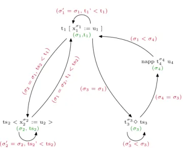
Table 1associates a lexicographical combination of structural orders to each function. We have written the types that are involved in the termination argument à la Church to make things clearer. Figure 1represents the call graph of the four functions:
• Each node corresponds to a function. We recall the lexicograph-ical orders described in Table 1 under the name of each func-tion.
• Each edge corresponds to a possible call of a function by an-other function. It is labelled with a summary of the correspond-ing call matrix (when a function calls itself, we add a prime symbol to the call arguments). In any circuit in the graph with starting and ending vertex s, the measure associated to s de-creases for the lexicographical order. It ensures that these mu-tual definitions terminate.
1The call matrices can be obtained by compiling our source file
Function t1[①1 σ1✿❂ ✉ 1] ts2❁ ①2 σ2 ✿❂ ✉ 2❃ Measure (σ1,t1) (σ2,ts2) Function t3 σ3 ✸ ts3 ♥❛♣♣ t4 σ4 ✉ 4 Measure (σ3) (σ4)
Table 1. Decreasing measures in hereditary substitutions
ts2<xσ22 := u2> (σ2, ts2) tσ3 3 ✸ ts3 (σ3) t1[ xσ11 := u1] (σ1,t1) napp tσ4 4 u4 (σ4) (σ 1 = σ2 ,t 1 < ts2 ) (σ 2 = σ1 ,ts 2 < t1) (σ′ 1= σ1, t1’ < t1) (σ3= σ1) (σ4= σ3) (σ′ 3< σ3) (σ1< σ4) (σ′ 2= σ2, ts2’ < ts2)
Figure 1. Call-graph in hereditary substitutions
3.5 Analyzing the normalizer
Once the definitions are established, the remainder of our devel-opment consists of an analysis of the normalizer in order to prove completeness and soundness (see Section 3.1). The next two sec-tions give some hints how to perform these proofs, with few details. One can consult the source code [2] for a higher level of detail.
In our context, the proofs in❆❣❞❛ mainly rely on two tech-niques, that we call generalization and the introduction of commu-tation lemmas. Only one proof presented in Section 5 needs special care.
3.5.1 Generalization
As all the functions are inductively defined, it is natural to conduct the proofs by induction as well. As a consequence, in order to prove a statement, we very often need to generalize over some variables appearing in it; otherwise, some of the induction cases are not provable.
For instance, we want to prove
❝♦♥❣❙✉❜st✬ : (t : ❚♠ (Γ, σ) τ) → ✉1βη✲≡ ✉2→
s✉❜st t ✈③ ✉1βη✲≡ s✉❜st t ✈③ ✉2
by induction overt. The variable and application cases do not pose any problem, but in the abstraction case, we would have to prove:
s✉❜st t (✈s ✈③) (✇❦❚♠ ✈③ ✉1) βη✲≡
s✉❜st t (✈s ✈③) (✇❦❚♠ ✈③ ✉2)
which does not ensue from the induction hypothesis. To make it work, we have to generalize over✈③ into:
❝♦♥❣❙✉❜st : (t : ❚♠ Γ τ) → (① : ❱❛r Γ σ) → ✉1βη✲≡ ✉2→s✉❜st t ① ✉1βη✲≡ s✉❜st t ① ✉2
3.5.2 Commutation lemmas
Most of the intermediary results we introduce are commutation lemmas. Informally, these are statements of the form❢ (❣ ①) ∼ ❣ (❢ ①)
where ∼ is either βη✲≡ or ≡. For instance, in order to prove com-pleteness (Section 4), we introduce the following lemma:
❝♦♠♣❆♣♣ : (t1 : ◆❢ Γ (σ ⇒ τ)) → (t2 : ◆❢ Γ σ) →
⌈♥❛♣♣ t1t2⌉ βη✲≡ ❛♣♣ ⌈ t1⌉ ⌈t2⌉
that states that embedding (⌈❴⌉) and application (♥❛♣♣ and ❛♣♣) commute.
4.
Proof of completeness
Completeness states that any term is βη-equivalent to its normal form. To show this property, we have to establish it for all the auxiliary functions that define♥❢ in Section 3.3: all these functions have to return a term that is βη-equivalent to their argument.
For the two functions that perform η-expansion, we have to prove the following properties:
Lemma 1. Theη-expansion of a termt is βη-equivalent to t: ♠✉t✉❛❧
❝♦♠♣◆❡ : (♥ : ◆❡ Γ σ) → ⌈ ♥❡✷♥❢ ♥ ⌉ βη✲≡ ❡♠❜◆❡ ♥ ❝♦♠♣❱❛r : (✈ : ❱❛r Γ σ) → ⌈ ♥✈❛r ✈ ⌉ βη✲≡ ✈❛r ✈ Proof.The two properties are proved by a mutual induction:
• over σ for❝♦♠♣◆❡; • using❝♦♠♣◆❡ for ❝♦♠♣❱❛r.
For the four functions that perform β-reduction, we have to prove commutation lemmas between the functions that define hereditary substitutions ( [❴✿❂❴], ❴❁❴✿❂❴❃, ✸ and ♥❛♣♣) and the functions that define the embedding from normal forms to terms (⌈❴⌉ and ❡♠❜❙♣):
Lemma 2. Hereditary substitutions and embeddings commute: ♠✉t✉❛❧ s✉❜st❊♠❜❙♣ : (ts : ❙♣ Γ τ ρ) → (① : ❱❛r Γ σ) → (t : ◆❢ (Γ ✲ ①) σ) → (❛❝❝ : ❚♠ Γ τ) → ❡♠❜❙♣ (ts ❁ ① ✿❂ t ❃) (s✉❜st ❛❝❝ ① ⌈ t ⌉) βη✲≡ s✉❜st (❡♠❜❙♣ ts ❛❝❝) ① ⌈ t ⌉ ❛♣♣◆❢❊♠❜❙♣ : (✉ : ◆❢ Γ σ) → (ts : ❙♣ Γ σ ◦) → ⌈✉ ✸ ts ⌉ βη✲≡ ❡♠❜❙♣ ts ⌈ ✉ ⌉ s✉❜st◆❢❙✉❜st : (t : ◆❢ Γ τ) → (① : ❱❛r Γ σ) → (✉ : ◆❢ (Γ ✲ ①) σ) → ⌈t [① ✿❂ ✉] ⌉ βη✲≡ s✉❜st ⌈ t ⌉ ① ⌈ ✉ ⌉ ❝♦♠♣❆♣♣ : (t1 : ◆❢ Γ (σ ⇒ τ)) → (t2 : ◆❢ Γ σ) → ⌈♥❛♣♣ t1t2⌉ βη✲≡ ❛♣♣ ⌈ t1⌉ ⌈t2⌉
Proof.The four properties are proven by a mutual induction: • overts for s✉❜st❊♠❜❙♣;
• overts for ❛♣♣◆❢❊♠❜❙♣; • overt for s✉❜st◆❢❙✉❜st; • overt1for❝♦♠♣❆♣♣.
We are now able to establish our main theorem:
Theorem 1(Completeness). Terms are convertible to their normal forms:
❝♦♠♣❧❡t❡♥❡ss : (t : ❚♠ Γ σ) → ⌈ ♥❢ t ⌉ βη✲≡ t
Proof.By induction overt using ❝♦♠♣❱❛r (Lemma 1) and ❝♦♠♣❆♣♣ (Lemma 2).
5.
Proof of soundness
Soundness states that the normalization function identifies two βη-equivalent terms. We are going to prove it by induction over the proof of βη-equivalence of the two terms.
This proof of soundness is longer than the proof of complete-ness, which is not really surprising since we have to provide a proof of equality, which is a relation more restrictive than the βη-equivalence. But we also get stuck on the generalization of one lemma, that makes us introduce a new predicate to be able to for-mulate it. We now explain the intuition about the reasons of the introduction of this predicate.
In order to prove soundness in the case wheret βη✲≡ ✉ is the rule❡t❛, we would like to show that, if ✉ is a normal form, then the η-expansion of✉ is equal to ✉:
❡t❛❊q : (✉ : ◆❢ Γ (σ ⇒ τ)) → λ♥ (♥❛♣♣ (✇❦◆❢ ✈③ ✉) (♥✈❛r ✈③)) ≡ ✉
As ✉ is a normal form which has a functional type, it is a λ-abstraction λ♥ t for a certain normal form t. So this lemma is equivalent to proving the following proposition:
Proposition 1.
(t : ◆❢ Γ τ) → ✇❦◆❢ (✈s ✈③) t [✈③ ✿❂ ♥✈❛r ✈③] ≡ t
As explained in Section 3.5.1, this proof must be performed by induction overt; and to be able to conclude in the inductive case wheret is an abstraction, we have to generalize over ✈③.
However, here, it is not as simple as in the example above: we are possibly misled by De Bruijn indices once more. We recall that the type of the function [① ✿❂ ✉] (described in section 3.3) states that if① is typed in a context Γ, then ✉ is typed in Γ ✲ ①. It means that in Proposition 1, the two occurrences of✈③ do not represent the same variable. In fact, they represent two consecutive variables in one context (which have the same type).
Hence, to generalize Proposition 1, it is necessary to general-ize the two occurrences of✈③ with two different names. But it is important to take into account the fact that they are consecutive, otherwise the lemma would not be correct. This is why we intro-duce a new predicate♦♥❡❞✐✛ that precisely identifies consecutive indices in one context.
5.1 The predicate onediff
This predicate is very simple to define by induction:✈③ and ✈s ✈③ follow one another; and if① and ② follow one another, then ✈s ① and ✈s ② too.
❞❛t❛ ♦♥❡❞✐✛ : ❱❛r Γ σ → ❱❛r Γ τ → ❙❡t ✇❤❡r❡ ♦❞③ : ♦♥❡❞✐✛ ✈③ (✈s ✈③)
♦❞s : (① : ❱❛r Γ σ) → (② : ❱❛r Γ τ) → ♦♥❡❞✐✛ ① ② →♦♥❡❞✐✛ (✈s ①) (✈s ②)
It is important to notice that ♦♥❡❞✐✛ satisfies the following property:
Lemma 3. If❥ and ✐ follow one another in Γ, then Γ ✲ ✐ and Γ ✲ ❥ are equal:
♦♥❡❞✐✛▼✐♥✉s : (✐ ❥ : ❱❛r Γ σ) → ♦♥❡❞✐✛ ❥ ✐ → Γ✲ ✐ ≡ Γ ✲ ❥
Proof. By induction over♦♥❡❞✐✛ ❥ ✐.
since it allows us to transform a variable, a term or a normal form ✉ typed in the context Γ ✲ ✐ into the same object typed in Γ ✲ ❥ for some Γ,✐ and ❥.
If♣ : Γ ≡ ∆ and ✉ is parameterized by Γ, then ! ♣ ❃ ✉ is ✉ parameterized by ∆. So, in the example above, if ♣✿ ♦♥❡❞✐✛ ❥ ✐, then the result of the transformation is !♦♥❡❞✐✛▼✐♥✉s ✐ ❥ ♣ ❃ ✉. 5.2 Theη-equality for normal forms
The predicate defined in the previous section now allows us to generalize Proposition 1 that way (detailed above):
Lemma 4.
s✉❜st◆❢❊q : (✐ : ❱❛r Γ τ) → (t : ◆❢ (Γ ✲ ✐) σ) → (❥ : ❱❛r Γ τ) → (❦ : ❱❛r (Γ ✲ ❥) τ) → (♣ : ♦♥❡❞✐✛ ❥ ✐) →✇❦✈ ✐ (! s②♠ (♦♥❡❞✐✛▼✐♥✉s ✐ ❥ ♣) ❃ ❦) ≡ ❥ → (✇❦◆❢ ✐ t) [❥ ✿❂ (♥✈❛r ❦)] ≡ ! ♦♥❡❞✐✛▼✐♥✉s ✐ ❥ ♣ ❃ t The intuition behind this statement is that we generalize in Proposition 1all the indices that appear:
(✇❦◆❢ ✐ t) [❥ ✿❂ (♥✈❛r ❦)] and add the two constraints:
• ♦♥❡❞✐✛ ❥ ✐: ❥ and ✐ are two consecutive indices;
• ✇❦✈ ✐ (! s②♠ (♦♥❡❞✐✛▼✐♥✉s ✐ ❥ ♣) ❃ ❦) ≡ ❥: ❥ and ✇❦✈ ✐ (! s②♠ (♦♥❡❞✐✛▼✐♥✉s ✐ ❥ ♣) ❃ ❦) represent the same variable.
These two conditions are sufficient to establish Lemma 4, and are verified by Proposition 1. Its proof only requires techniques presented in Section 3.5.
The η-equality for normal forms is now a direct consequence of s✉❜s◆❢❊q:
Lemma 5. Theη-equality is true for normal forms: ❡t❛❊q : (✉ : ◆❢ Γ (σ ⇒ τ)) →
λ♥ (♥❛♣♣ (✇❦◆❢ ✈③ ✉) (♥✈❛r ✈③)) ≡ ✉ ❡t❛❊q (λ♥ ✉) =
r❡✢λ♥ (s✉❜st◆❢❊q (✈s ✈③) ✉ ✈③ ✈③ ♦❞③ r❡✢) 5.3 Theβ-equality for normal forms
Similarly to completeness, to prove soundness in the case where βη✲≡ is ❜❡t❛, we have to prove the following commutation lemma: Lemma 6. Normalization and substitution commute:
♥❢❙✉❜st◆❢ : (t : ❚♠ Γ τ) → (① : ❱❛r Γ σ) → (✉ : ❚♠ (Γ ✲ ①) σ) → (♥❢ t) [① ✿❂ (♥❢ ✉)] ≡
♥❢ (s✉❜st t ① ✉)
The proof is a rather technical but uses techniques presented in Section 3.5.
5.4 Proof of soundness
We are now able to establish our main theorem:
Theorem 2(Soundness). The normal forms of two convertible terms are equal:
s♦✉♥❞♥❡ss : {t ✉ : ❚♠ Γ σ} → t βη✲≡ ✉ → ♥❢ t ≡ ♥❢ ✉
Proof.By induction overt βη✲≡ ✉, using ❡t❛❊q (Lemma 5) in the ❡t❛ case and and ♥❢❙✉❜st◆❢ (Lemma 6) in the ❜❡t❛ case. The other cases are trivial.
Conclusion of Sections 4 and 5: The reverse of Theorem 2 (soundness) is a direct consequence of Theorem 1 (completeness):
Consequence 1. Two terms whose normal forms are equal are convertible.
❝♦♥✈❡rt♥❢ : (t ✉ : ❚♠ Γ σ) → ♥❢ t ≡ ♥❢ ✉ → t βη✲≡ ✉ It follows that two terms are βη-equivalent if and only if their normal forms are equal. As equality on normal forms is obviously decidable, we can conclude that βη-equivalence is decidable.
Moreover, we expect that our algorithm that decides equiva-lence (normalize and check the equality of normal forms) uses only first order primitive recursion. We did not prove it formally, but it seems reasonable to say that it follows from construction. It makes clear that βη-equivalence is primitive recursive.
6.
Related work
Hereditary substitutionswere first introduced by Watkins et al. [17] to define a normalizer for the Concurrent Logical Frame-work. Their property to preserve canonical forms during substitu-tion makes them a nice approach to an implementasubstitu-tion of substi-tutions for Logical Frameworks [9, 12] and Higher-Order Abstract Syntax [15]. Abel [3] already noticed that the fact that hereditary substitutions are structurally recursive makes it easy to automati-cally check the termination of the algorithm they provide. We ex-ploit the two properties:
•The fact that canonical forms are preserved by hereditary sub-stitutions ensures the correct typing given to the substitution function.
•The fact that it is structurally recursive allows us to implement it in❆❣❞❛ without any need of an explicit termination proof. The lemmas presented in this paper do not bring something new by their statements, but by their proofs. In fact, hereditary substitutions were studied in many different contexts [5, 12, 14], and most of our theorems are already proved in those papers. The main difference is that they use a named representation of variables.
Indeed, one major contribution of this paper is to adapt hered-itary substitutions to De Bruijn indices (with the drawbacks we know, but with advantage that due to the fact that closed terms have a unique representation) and to implement it in an interactive theo-rem prover based on Type Theory.
Using dependant types in order to define directly the set of well-typed terms is not new. Its formalization has been studied in different interactive theorem provers based on dependant types, such as❆❣❞❛ [7] and ❈♦q [8].
Also related is David’s work on arithmetical proofs of normal-ization results, e.g. see [10]. Besides, [6] uses big step normaliza-tion to show decidability of a substitunormaliza-tion calculus - this work has also been formalized in❆❣❞❛.
7.
Conclusion
This paper implements in❆❣❞❛ a normalizer for the simply typed λ-calculus, and proves that this normalizer can be used to decide the βη-equality over terms. It exploits some aspects of❆❣❞❛ and, more generally, of programming languages with dependent types:
•Dependent types are not only used to express theorems’ state-ments, but also serve to define particular sets. Here, the parame-terization of variables, terms and normal forms by contexts and types is a useful and natural way to define only the subset of λ-terms we are interested in. It is important to notice that❆❣❞❛’s implementation of dependent types makes it straightforward to manipulate such objects.❆❣❞❛’s dependent typing also ensures properties about functions just “by definition”.
• ❆❣❞❛’s termination checker is powerful enough to analyze non trivial mutually inductive definitions.
• Conversely, hereditary substitutions give a nice way to define a normalizer within total Type Theory, without constructing a proof of termination of a partial function. This could be ex-tended to more complex type systems, for instance with poly-morphism [3].
Acknowledgments
We thank Conor McBride, who suggested the idea and introduced some very convenient notations such as Γ ✲ ①. We also thank Andreas Abel for his useful help and comments about hereditary substitutions. We are grateful to the anonymous reviewers for their accurate comments and suggestions.
References
[1] Agda wiki.❤tt♣✿✴✴✇✐❦✐✳♣♦rt❛❧✳❝❤❛❧♠❡rs✳s❡✴❛❣❞❛.
[2] The decidability of the βη-equivalence using hereditary substitutions. ❤tt♣✿✴✴✇✇✇✳❧✐①✳♣♦❧②t❡❝❤♥✐q✉❡✳❢r✴⑦❦❡❧❧❡r✴❘❡❝❤❡r❝❤❡✴ ❤s✉❜st✳❤t♠❧.
[3] A. Abel. Implementing a normalizer using sized heterogeneous types. Workshop on Mathematically Structured Functional Programming, MSFP, 2006.
[4] A. Abel and T. Altenkirch. A predicative analysis of structural recur-sion. J. Funct. Program., 12(1):1–41, 2002.
[5] A. Abel and D. Rodriguez. Syntactic Metatheory of Higher-Order Subtyping. In M. Kaminski and S. Martini, editors, CSL, volume 5213 of Lecture Notes in Computer Science, pages 446–460. Springer, 2008. ISBN 978-3-540-87530-7.
[6] T. Altenkirch and J. Chapman. Tait in one big step. In Workshop on Mathematically Structured Functional Programming, MSFP, volume 2006. Citeseer, 2006.
[7] T. Altenkirch and B. Reus. Monadic Presentations of Lambda Terms Using Generalized Inductive Types. In J. Flum and M. Rodríguez-Artalejo, editors, CSL, volume 1683 of Lecture Notes in Computer Science, pages 453–468. Springer, 1999. ISBN 3-540-66536-6. [8] N. Benton, A. Kennedy, and C. Hur. Strongly typed term
representa-tions in Coq.
[9] K. Crary. Explicit Contexts in LF (Extended Abstract). Electr. Notes Theor. Comput. Sci., 228:53–68, 2009.
[10] R. David. Normalization without reducibility. Annals of pure and applied logic, 107(1-3):121–130, 2001.
[11] N. G. De Bruijn. Lambda Calculus Notation with Nameless Dummies: a Tool for Automatic Formula Manipulation With Application to the Church-Rosser Theorem. Indag. Math., pages 381–382, 1972. [12] R. Harper and D. R. Licata. Mechanizing metatheory in a logical
framework. J. Funct. Program., 17(4-5):613–673, 2007.
[13] U. Norell. Towards a Practical Programming Language Based on Dependent Type Theory. PhD thesis, Chalmers Univ. of Tech., 2007. [14] F. Pfenning. Church and Curry: Combining intrinsic and extrinsic
typing. Studies in Logic and the Foundations of Mathematics, 2008. [15] B. Pientka. A type-theoretic foundation for programming with
higher-order abstract syntax and first-class substitutions. In G. C. Necula and P. Wadler, editors, POPL, pages 371–382. ACM, 2008. ISBN 978-1-59593-689-9.
[16] B. Pierce. Types and programming languages. The MIT Press, 2002. Chapter 12: Normalization.
[17] K. Watkins, I. Cervesato, F. Pfenning, and D. Walker. A Concur-rent Logical Framework: The Propositional Fragment. In S. Berardi, M. Coppo, and F. Damiani, editors, TYPES, volume 3085 of Lecture Notes in Computer Science, pages 355–377. Springer, 2003. ISBN 3-540-22164-6.