On the statistical distribution of first-return times of balls and cylinders in chaotic systems

HAL Id: hal-00476239

https://hal.archives-ouvertes.fr/hal-00476239

Submitted on 25 Apr 2010

HAL is a multi-disciplinary open access

archive for the deposit and dissemination of

sci-entific research documents, whether they are

pub-lished or not. The documents may come from

teaching and research institutions in France or

L’archive ouverte pluridisciplinaire HAL, est

destinée au dépôt et à la diffusion de documents

scientifiques de niveau recherche, publiés ou non,

émanant des établissements d’enseignement et de

recherche français ou étrangers, des laboratoires

On the statistical distribution of first-return times of

balls and cylinders in chaotic systems

Sandro Vaienti, Giorgio Mantica

To cite this version:

Sandro Vaienti, Giorgio Mantica. On the statistical distribution of first-return times of balls and

cylinders in chaotic systems. International journal of bifurcation and chaos in applied sciences and

engineering , World Scientific Publishing, 2010, 20 (6), pp.1845. �10.1142/S0218127410026897�.

�hal-00476239�

On the statistical distribution of first–return

times of balls and cylinders in chaotic systems

G.Mantica

_{, and S.Vaienti}

Abstract

We study returns in dynamical systems: when a set of points, initially populating a prescribed region, swarms around phase space according to a deterministic rule of motion, we say that the return of the set occurs at the earliest moment when one of these points comes back to the origi-nal region. We describe the statistical distribution of these “first–return” times in various settings: when phase space is composed of sequences of symbols from a finite alphabet (with application for instance to biological problems) and when phase space is a one and a two-dimensional man-ifold. Specifically, we consider Bernoulli shifts, expanding maps of the interval and linear automorphisms of the two dimensional torus. We de-rive relations linking these statistics with R´enyi entropies and Lyapunov exponents.

1

Introduction

In this paper we investigate a phenomenon of vast relevance in physics: returns. Whenever a system evolves according to a deterministic, or even a probabilis-tic law, along the course of time it may pass close to points previously visited. We then speak of returns and of return times. Of course, this concept can be made precise and rigorous: this has been done since the beginning of the theory of dynamical system, where Poincar´e theorem—establishing that in measure preserving systems returns happen almost surely—is probably the first and cer-tainly the most celebrated result. Passing via Kac theorem and coming to recent years, mathematical investigation has flourished and produced beautiful results relating the statistics of return times, i.e. the collective counting of these values, to more conventional dynamical indicators, such as generalized dimensions of invariant measures, Lyapunov exponents and the like. This paper continues in this ongoing investigation, with a special character: rather than presenting a

∗_{International Center for Non-linear and Complex Systems, Universit`a dell’Insubria, Via}

Vallegio 11, Como, and CNISM, unit`a di Como, I.N.F.N. sezione di Milano, Italy E-mail: <giorgio@uninsubria.it>.

†_{Centre de Physique Th´eorique, UMR 6207, CNRS, Luminy Case 907, F-13288 Marseille}

Cedex 9, and Universities of Aix-Marseille I, II and Toulon-Var. F´ed´eration de Recherche des Unit´es de Math´ematiques de Marseille, France. E-mail: <vaienti@cpt.univ-mrs.fr>.

single, thoroughly investigated result, we attempt to provide a heuristic, global picture of the dynamical phenomena that are at work. This picture will be con-firmed by numerical experiments. Rigor and complete proofs will be the matter for successive publications.

There exist many different alternatives when defining returns: in this paper, we make specific reference to what is called the first return of a (measurable) subset A of a compact metric space, endowed with a measure µ defined on the Borel sigma algebra A. Motion on X is effected by the action of a transformation

T that preserves the measure µ. We thereby define the time of first return of A

into itself as

τ (A) := min{k > 0 s.t. TkA ∩ A 6= ∅} . (1) As anticipated in the abstract, this is the time of the earliest return to A of one of its points:

τ (A) = min{k > 0 s.t. ∃x ∈ A; Tk_{(x) ∈ A}. (2)} Two choices will be made for A. Firstly, A shall be a ball of radius ε, centered at a point x ∈ X: Bε(x). Secondly, A shall be a dynamically generated cylinder. Let us suppose that C is a finite partition of X and take the n-join,

Cn _{:= ∨}n−1

i=0T−iC. We call cylinder of length n around x ∈ X, denoted with

Cn(x), the unique element of Cncontaining x. The statistics of return times are then defined by the collective counting, over different sets, of the values τ (A). The distribution of return times, p(ε, k) is

p(ε, k) := µ({x ∈ X s.t τ (Bε(x)) = k}); (3) similarly, p(n, k) is defined replacing Bε(x) by Cn(x). They measure the fraction of points in the space X whose neighborhood (whether a ball, or a cylinder, of fixed radius ε or length n) first returns to itself after k iterations of the map. We shall also consider the cumulative distributions (integrated statistics) P (ε, k),

P (ε, k) :=

k X j=1

p(ε, j) (4)

and P (n, k). Our aim will be to study the behavior of these distributions in systems that are simple enough to permit both a theoretical analysis and a precise numerical simulation.

The time of first return of sets (1) arises in several circumstances. Since it controls the shortest return time of points in the set, it plays a crucial role to establish the asymptotic (exponential) distribution of the return times of all points to the set A, when the measure of the set A goes to zero, a different and much investigated topic [16, 3, 1, 2, 22, 20, 19]. In addition, it has been used to define the recurrence dimension, being used as the gauge set function to construct a suitable Carath´eodory measure [5, 25, 7]. Finally, it has been related to the algorithmic information content [11].

Returns of sets is also relevant in applications, like those of biological interest. In fact, when the space X consists of sequences of symbols from a finite alphabet

(think e.g. of DNA sequencing) particular words, or motifs have been found to be related to biological mechanisms like transcription sites or protein interaction (see for instance [28]). It is then important to quantify the statistical properties of these words within the genome. In particular, a typical word of length n (that is, a finite sequence of n letters) will recur within a time of the order enh_, for large n, where h is the metric entropy of the system, as predicted by the Ornstein-Weiss theorem [23]. Yet, if we look at the delay of the first recurrence of the same word, when observed in the whole (possibly infinite) sequence, this scales as n [29, 6]. This time of first return is precisely the quantity studied in this paper.

The plan of the paper is the following: in the next section we review a few results that are useful for the understanding of the paper. For this reason we neither claim nor need completeness. In Sect. 3 we consider the case of cylinder return times in Bernoulli systems. Quite evidently, this is the simplest setting where to study return times of sets. We first present a heuristic explanation of the results rigorously proven in [4] and [21] that permit to compute, via return times, the R´enyi entropies. Then, we refine this analysis to obtain new results on the type of convergence of the conventional quantities and we introduce a new one, for which convergence is much faster. Moreover, our theory allows us to obtain a description of the different asymptotics of p(n, k) in the (n, k) plane. In Sect. 4 we leave the symbolic description to enter a geometric setting by considering expanding maps of the interval. We show how results proven in the symbolic setting can be adapted to describe the behavior of the distribution function p(ε, k). While the treatment is here tailored on the specific system under investigation, the following Sect. 5 introduces a more general approach. Here, we derive a relation linking return times and a partition function that yields R´enyi entropies in a suitable limit. In Sect. 6 we consider the case of linear automorphisms of the two-dimensional torus, that can be investigated completely. We also conjecture a general form for one of the asymptotics of the return times statistics. In the Conclusions we review the new results presented in this paper.

2

Review of known results and definitions

Many facts concerning return times of sets are known. In this section we review a few of these results that are relevant for the understanding of this paper. If the dynamical system (X, µ, T ) has positive metric entropy, hµ, it has been proven [29, 6] that:

lim inf n→∞

τ (Cn(x))

n ≥ 1 . (5)

The above limit exists and is equal to one µ-almost everywhere in certain cases, including irreducible and aperiodic subshifts of finite type, systems veri-fying the specification property [6] and even non-uniformly hyperbolic maps of the interval [22, 15]. It is therefore of importance to study the measure of the set of points that deviate from the almost-sure behavior, a quantity that typically

decays exponentially in time. To do this precisely, one defines the deviation function M (δ), M (δ) := lim n→∞ 1 nlog µ({x ∈ X s.t τ (Cn(x)) n < δ}). (6)

In the language of the previous section this becomes

M (δ) = lim

n→∞ 1

nlog P (n, δn) (7)

In [4] it has been proven that, for ψ-mixing dynamical systems with some restrictions (see the original paper for definition and further specifications) the limit above exists and is related to the generalized R´enyi entropies H of the invariant measure µ via

M (δ) = (δ − 1)H(1

δ − 1), (8)

whenever the latter function exists, being it defined via a summation over all cylinders C of length n, H(β) := −1 β n→∞lim 1 nlog X C∈Cn µ(C)β+1_{. (9)}

Observe that meaningful values of δ in eq. (6) range from zero to one, so that

β = 1

δ − 1 is always larger than zero. For non-integer values of 1δ, a linear interpolation of the values provided by eq. (8) applies.

R´enyi entropies have been introduced in [27] and they have been extensively studied in the eighties for their connections with various generalized spectra of dimensions of invariant sets, see for instance [18, 9, 14, 10, 17, 13, 24, 31, 32]. The restrictions in [4] have been removed in [21] and in this last paper the R´enyi entropies have been proved to exist for a weaker class of ψ-mixing measures.

On the other hand, one might try to answer similar questions when balls are considered in place of cylinders. For instance, if Bε(x) is the ball of radius ε centered at x ∈ X, the natural generalization of the limit (5) is the quantity

η(x) := lim

ε→0+

τ (Bε(x))

− log ε . (10)

For a large class of maps of the interval, it has been proved in [29] that η(x) exists for µ-almost all x and is equal to the inverse of λ, the Lyapunov exponent of the measure µ. For hyperbolic smooth diffeomorphisms of a compact manifold a similar result holds, to the extent that

1

Λu ≤ lim inf_ε→0

τ (Bε(x))

− log ε ≤ lim supε→0

τ (Bε(x))

− log ε ≤

1

λu, (11) where Λu _{and Λ}s _{are the largest and the smallest Lyapunov exponents, while}

Lyapunov exponent, see [30]. In the case of diffeomorphisms in two dimensions, the above formula leads to the equality

lim ε→0 τ (Bε(x)) − log ε = 1 Λu − 1 Λs = 1 λu− 1 λs = D1(µ) hµ . (12) The last equality above is Young’s formula, in which D1(µ) is the information

dimension and hµ is the metric entropy of the measure µ. One of the goals of this paper is to generalize the results (7), (8) in the case of balls.

3

Return times in Bernoulli shifts

In this section we take a close look at Bernoulli processes, that are the simplest, yet significant, example of ψ-mixing systems. For these, eq. (8) holds and the function H can be easily computed. In our view, this result is particularly significant, because it allows us to compute a thermodynamical quantity, the spectrum of R´enyi entropies, from the statistics of return times. Our aim is to investigate the kind of convergence holding for eq. (7) and more generally the form of the distribution p(n, k). We shall also introduce a slightly different quantity than P (n, δn), still based on return times, that also yields M (δ) in the limit, but for which convergence is much faster.

Let us start from notations: we consider the full shift on the space of se-quences of M symbols, Σ := {0, . . . , M − 1}Z+_{. Let us stipulate that the}

cylinders in Cn _{can be written as C}

σ0,...,σn−1, where σi ∈ {0, . . . , M − 1}, for

i = 1, . . . , n − 1. For short, we shall sometimes write σ for the vector of indices σi, and |σ| will be the length of this vector. σ is also called a “word” in symbolic language. With a slight abuse of notation, we shall sometimes write τ (σ) and

µ(σ), the return time and the measure of the word σ, in place of τ (Cσ) and

µ(Cσ), the return time and the measure of the cylinder Cσ labeled by the word

σ. Similarly, we shall let Σn := {0, . . . , M − 1}n indicate the set of words of length n and Cn _{the set of the associated cylinders, at times interchangeably.}

The Bernoulli invariant measure on Σ is induced by the set of probabil-ities {πj}, j = 0, . . . , M − 1. For simplicity, in the numerical simulations, we shall consider the two-symbols (coin toss) Bernoulli game of parameter q:

π0= q, π1= 1 − q.

Fig. 1 depicts the function p(n, k) for q = 0.3. Two features are evident: the first, is the slow decay of p(n, 1) with increasing n. The second is the much faster decay of p(n, 2). Both these features, and more, can be explained by computing the asymptotic behavior of p(n, k) for k fixed and large n.

The case k = 1 follows immediately from the observation that the only words

σ for which τ (σ) = 1 are composed of a single symbol: σi = j for all i, where

j ∈ {0, . . . , M − 1}. The measure of the associated cylinders is πn

j, so that

p(n, 1) is the sum of these quantities over all j, and behaves asymptotically as an_{, where a = max{π}

j}.

Let now Tn,k the set of words of length n with first return time k:

-20 -18 -16 -14 -12 -10 -8 -6 -4 -2 0 0 5 10 15 20 25 6 8 ₁₀ 12 ₁₄ 16 ₁₈ 20 ₂₂ 24 ₂₆ -20 -18 -16 -14 -12 -10 -8 -6 -4 -2 0 log(p(n,k)) k n log(p(n,k))

Figure 1: Distribution function p(n, k) for the Bernoulli game with q = 0.3. The first observation is that for any σ ∈ Tn,k the symbols σi repeat periodically with period k:

σk+j= σj, j = 0, . . . , n − k. (14) Define the periodic replication operator Pn,k_{as that which takes any word σ of} length k into the word σ0_{= P}n,k_{(σ) of length n ≥ k, that satisfies eq. (14). It} is of relevance now to consider the set of words Wn,k defined implicitly by

Tn,k= Pn,k(Wn,k). (15) The meaning of this definition is simple: words in Wn,k have length k and are all and the only periodic “roots” of words of Tn,k:

Wn,k = {σ ∈ Σk s.t. τ (Pn,k(σ)) = k}. (16)

Controlling Wn,k is then the same thing as controlling Tn,k. It is not difficult to prove that for any k

Tk,k= Wk,k⊂ Wk+1,k⊂ . . . W2k,k= W2k+1,k= . . . = W2k+j,k, (17)

for any j ≥ 0. Therefore, when n ≥ 2k the set of “roots” Wn,k is constant in n. Define

m(k) = max

σ∈W2k,k

{#{j s.t. σj= 0}}. (18) This is the maximum number of zeros in a word in W2k,k. Since all sets Wn,k are invariant for permutation of the symbols {0, . . . , M − 1}, m(k) is also the

maximum number of any other symbol in a word in W2k,k. Suppose now that

only one symbol in {0, . . . , M − 1} has probability a, so that the probability of all other symbols is less than a. For simplicity, let us only consider the case of

M = 2. Then, the probability of the word for which m(k) is obtained gives the

leading term in the asymptotic of p(n, k): log(p(n, k)) ∼ n

k[m(k) log a + (k − m(k)) log(1 − a)]. (19)

It is also rather easy to see that m(k) = k − 1. In fact, m(k) = k is possible only for k = 1, and σk−1= 1, σj = 0 for j = 0, . . . , k − 2 is a word in W2k,k.

Then, 1 nlog(p(n, k)) ∼ (1 − 1 k) log a + 1 klog(1 − a). (20)

This formula gives the decay rates of p(n, k). They are increasing functions of

k ≥ 2, the most negative being precisely that of p(n, 2), and tend to log(a) when k goes to infinity.

Let us now consider the asymptotic behavior of p(n, k) over the line k = δn, where 0 < δ < 1. Firstly, it is clear that Wn,k 6= Σk, since some words of length

k may be associated with shorter return times than k, and one the technical

achievements of refs. [4, 21] is to deal properly with this issue. This fact notwithstanding, we may begin by assuming heuristically that among all words

σ in Σk, those associated with return times smaller than k and therefore not in Wn,k, are statistically negligible, in some limit. More refined arguments will follow later in this section. Under this assumption, the probability p(n, k) can be approximated by a sum over all words of length k:

p(n, k) = X

σ∈Wn,k

µ(Pn,k_{(σ)) '} X

σ∈Σk

µ(Pn,k_{(σ)). (21)}

Formula (21) can be further developed by estimating the cylinder measure µ(σ0_), where σ0_{= P}n,k_{(σ). Since |σ| = k, |σ}0_{| = n, and since σ}0 _{satisfies eq. (14),}

log µ(σ0) = n

klog µ(σ), (22)

exactly whenevern

k is an integer (and approximately in the other cases) so that

p(n, k) = X

σ∈Σk

µ(Cσ)n/k. (23)

If we now set k = δn, with 0 < δ ≤ 1 and δ the inverse of an integer, we can estimate lim n→∞ 1 nlog p(n, δn) = δ limk→∞ 1 klog( X σ∈Σk µ(Cσ)1/δ). (24)

If we now compare this equation with the definition of R´enyi entropies, eq. (9), we easily obtain that

M (δ) = lim n→∞ 1 nlog p(n, δn) = (δ − 1)H( 1 δ − 1). (25)

Observe that this heuristic result has been derived for p(n, k) rather than

P (n, k), for which it is known to hold rigorously–modulo the linear

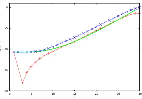
interpola-tion required for non-integer values of 1/δ. Indeed, numerical experiments on Bernoulli schemes with two symbols (coin toss) show that formula (25) holds. For instance, Figure 4 shows the logarithm of both p(n, δn) and P (n, δn) versus

n, for q = 0.3 and δ = 0.5, compared with a straight line gδ(n) = an + b with slope a = (δ − 1)H(1

δ − 1). Both quantities are well fitted by a function of the kind gδ(n) + cedn.

To validate this picture, confirmed by numerical experiment on other values of q and δ (for δ not equal to the inverse of an integer, a linear interpolation formula applies [4, 21]) we plot in Fig. 5 the logarithm of the difference between data and the straight line in Fig. 4. An exponential decay is clearly observed.

In conclusion, numerical experimentation support the hypothesis that the asymptotic behavior in eq. (25) is attained with a decaying exponential term parameterized by the constants c and d < 0, together with a slowly decaying contribution arising from the constant b:

1 nlog p(n, δn) ' M (δ) + b n+ c ne dn_{. (26)}

We shall introduce momentarily a new quantity to improve on this kind of convergence.

The same heuristic arguments imply an approximate form for the behavior of the distribution function for different n and k. Carrying out the computations of eq. (23) together with eq. (9) we obtain

log(p(n, k)) ∼ (k − n)H(n

k− 1). (27)

We can test this approximation in the case of the Bernoulli scheme with

q = 1/2. Here, trivially the approximation (27) becomes log(p(n, k)) ∼ (k − n) log(2)). This function fits almost perfectly the numerical data in Fig. 2.

A less favorable case is offered by the Bernoulli scheme with q = .3. In Fig. 3 we plot P (n, k) and p(n, k) versus k for n = 30, together with the approximation provided by eq. (27) We notice that this latter fits well both functions at k = 1 (quite obviously, being this behavior associated with the measure of the cylinder of unity return time, see above), while approximation stays reasonable only for

P (n, k) at small values of k > 1. Then, in the intermediate region the slope

of both curves agrees with the interpolation while the numerical value only for

p(n, k).

Certainly, the agreement observed in the last figure is far from satisfactory. The reason is to be found in the approximation made in eq. (21). The same fact is at the origin of the slow convergence observed in eq. (26). We con-clude this section unveiling these reasons and providing a more rigorous and insightful treatment of the problem. This improvement is inspired by the idea of summation over prime periodic orbits in dynamical systems.

As we mentioned, the approximation in eq. (21) above is based on the idea that the roles of Σkand Wn,k can be interchanged, the effects of their difference

0 5 10 15 20 25 30 5 10 15 20 25 30 -20 -15 -10 -5 0 log p(n,k) k n log p(n,k)

Figure 2: Distribution function p(n, k) (crosses, red lines) and the approximation function in eq. (27) (x, green line) versus n and k in the case of a Bernoulli game with q = 1/2.

being negligible in the limit. The price to pay in this procedure is the slowly decaying term in the asymptotics (26). We can be more careful: indeed, we can show that Σk can be rigorously partitioned into the periodic repetition of

different sets Wn,k0. The lemma is the following: for any n ≥ 2k

Σk= [

k0_|k

Pk,k0

(Wn,k0), (28)

where the union is over all integer k0_{that divide k and where the sets P}k,k0

(Wn,k0)

are the full completion of k

k0 cycles of the word of length k0. These sets are

pair-wise disjoint.

On the basis of this lemma, we can reverse the ordering in eq. (21) to get: X σ∈Σk µ(Pn,k(σ)) =X k0_|k X σ∈W_n,k0 µ(Pn,k◦ Pk,k0(σ)). (29) Since k0 _{divides k, P}n,k _{◦ P}k,k0 = Pn,k0

and therefore the chain of equality continues with X σ∈Σk µ(Pn,k(σ)) =X k0_|k X σ∈W_n,k0 µ(Pn,k0(σ)) =X k0_|k X σ∈T_n,k0 µ(σ), (30)

-20 -15 -10 -5 0 0 5 10 15 20 25 30 log p(n,k) k

Figure 3: Distributions P (n, k) (X, blue line), p(n, k) (crosses, red line) and the approximation function in eq. (27) (green line) versus k for n = 30, in the case of a Bernoulli process with q = 0.3

where we have used eq. (15). Finally, X σ∈Σk µ(Pn,k_{(σ)) =}X k0_|k X σ∈Tn,k0 µ(σ) =X k0_|k p(n, k0_{). (31)}

On the other hand,

µ(Pn,k(σ)) = (µ(Cσ)) n

k, (32)

exactly when n

k is an integer, and approximately otherwise, so that choosing

k/n = δ, so that δn = k is an integer, and defining the new quantity Zp(δ, n) := X k0_|δn p(n, k0_{), (33)} we find that Mp(δ) = lim_n→∞1 nlog(Zp(δ, n)) = (δ − 1)H( 1 δ − 1). (34)

This formula is valid for all 0 < δ ≤1

2 that are the inverse of an integer. For the

other values, the linear interpolation between the values at the nearest inverses of an integer applies.

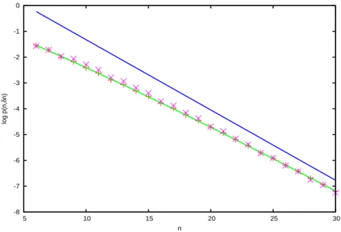
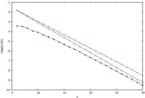
Numerical verification follows: in Fig. 6 we plot the logarithm of P (n, δn),

-8 -7 -6 -5 -4 -3 -2 -1 0 5 10 15 20 25 30 log p(n, δ n) n

Figure 4: Distribution function p(n, δn) for a Bernoulli process with q = 0.3,

δ = 0.5 (X) and cumulative distribution function P (n, δn) of the same process

(crosses). The first function has been shifted upwards by a fixed quantity to match the latter. Both sets of data are consistent with the behavior described in the text: The straight blue line has indeed slope (δ − 1)H(1

δ − 1), and the green fitting curve (which becomes asymptotically tangent to the blue line) is given by eq. (26).

process with q = 0.3. The line gδ(n) = M (δ)n fits almost perfectly the last set of data. On the other hand, the other two functions display the slow convergence discussed above. To further appreciate the improvement brought about by using

Zpconsider Fig. 7, where we plot the difference between successive values of the logarithm of the above functions, and these logarithms divided by n. All these quantities have limit M (δ). We compute this value from the linear interpolation of (δ−1)H(1

δ−1) to get the value tabulated. The distributions p and P converge slowly, while Zp gives a numerically exact result. In conclusion, the term b > 0 plaguing the convergence in eq. (26) was do to approximate counting and does not show up for the newly introduced quantity.

4

Expanding maps of the interval

In this section, we study a family of one-dimensional dynamical systems for which we can derive both a formula for the asymptotic distribution and a gen-eralization of the deviation result. This family will also serve to begin to under-stand the dynamical phenomena occurring when considering ball, rather than

-1 -0.8 -0.6 -0.4 -0.2 0 0.2 0.4 5 10 15 20 25 30 log (g δ (n) - log(P(n, δ n)) n

Figure 5: Logarithm of the difference between the logarithm of the cumulative distribution function P (n, δn) of the Bernoulli process with q = 0.3, δ = 0.5 and the straight line gδ(n) in Fig. 4. The fitting straight (green) line implies the exponential decay used in the fit in Fig. 4.

cylinder, return times: one has to match geometry and dynamics. Further detail will be added in the following section.

We start by constructing a family of measures supported in [0, 1] by means of an affine iterated function system: given a set of M non-overlapping intervals

Ij = [aj, bj] ⊂ [0, 1] j = 0, . . . , M − 1, define the lengths δj = bj − aj, and construct the affine maps

φj(x) := δjx + aj, j = 1, . . . , M. (35) Each map φj takes [0, 1] into [aj, bj]. Consider then the set action Φ that maps the set A ⊂ [0, 1] into Φ(A) := SM −1_j=0 φj(A). Repeated action of Φ on [0, 1] defines a Cantor set S in [0, 1]:

S :=

∞ \ k=1

Φk_{([0, 1]). (36)}

We can then construct a family of measures whose support is this set S: let us choose real numbers {πj}j=1,...,M such that πj > 0,

PM

j=1πj = 1, and consider the unique measure µ for which

Z f (s)dµ(s) = M −1_X j=0 πj Z (f ◦ φj)(s)dµ(s), (37)

-10 -9 -8 -7 -6 -5 -4 -3 -2 -1 5 10 15 20 25 30 log(p(n, δ n)) n

Figure 6: Logarithm of the cumulative distribution function P (n, δn) (red line, pluses) and of the distribution function p(n, δn) (blue line, stars) together with log Zp(δ, n) (large crosses, light blue) and the line gδ(n) = M (δ)n (magenta) for the Bernoulli process with q = 0.3, δ = 0.4

holds for any continuous function f . It is then easy to show that, for any choice of the set of real numbers {πj}, the measure µ is mixing for the piece-wise linear transformation T defined on S by:

T (x) = aj+ 1

δj

(x − aj), if x ∈ Ij= [aj, bj]. (38)

In fact, the maps {φj} turn out to be the inverse branches of T . As such, they can be employed to build the cylinders Cn _{of this dynamical system: letting}

σi∈ {0, . . . , M − 1}, for i = 1, . . . , n − 1 these latter can be labelled as

Cσ0,...,σn−1= (φσ0◦ · · · ◦ φσn−1)([0, 1]). (39)

Following eq. (35), the geometric length `(Cσ) is easily computed:

`(Cσ0,...,σn−1) =

n−1_Y

i=0

δσi. (40)

Equally easily, because of eq. (4), the measure µ(Cσ) is

µ(Cσ0,...,σn−1) =

n−1_Y

i=0

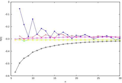
-0.6 -0.5 -0.4 -0.3 -0.2 -0.1 0 5 10 15 20 25 30 h(n) n

Figure 7: Various functions for of the Bernoulli process with q = 0.3, δ = 0.4. Start with log(p(n, δn))/n: black curve, circles; log(p(n, δn))−log(p(n−1, δ(n− 1)): blue curve, stars; log(P (n, δn))/n open squares, magenta; log(P (n, δn)) − log(P (n − 1, δ(n − 1))): crosses, red curve; log(Zp(n, δ))/n: yellow squares; log(Zp(n, δ)) − log(Zp(n − 1, δ)): crosses, green curve. The last two set of data sit to numerical precision on the line h = −0.307795889757108 that is obtained by the interpolation formula.

Therefore, this dynamical system is metrically equivalent to a Bernoulli shift on M symbols, with probabilities πi, i = 1, . . . , M − 1, that we have discussed in section 3. Yet, when examining the distribution of ball return times, we must investigate is the geometrical relation between balls of a fixed radius and cylinders of different symbolic length.

In order to analyze this relation, we observe that any ball Bε(x) can be written as a union over cylinders of an appropriate (fixed) length n: that is, for all x and ε there exist n and a collection of indices σ ∈ I, |σ| = n such that

Bε(x) = [ σ∈I

Cσ. (42)

This is a consequence of the fact that these measures are singular w.r.t. Lebesgue and their support have gaps of positive length. Therefore, for suffi-ciently large n, the two boundary points of the ball end up in the closure of a gap in the support of µ.

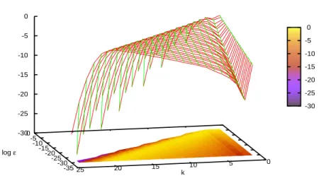
-30 -25 -20 -15 -10 -5 0 k log ε -30 -25 -20 -15 -10 -5 0 log p(ε,k) 0 5 10 15 20 25 -35 -30 -25 -20 -15 -10 -5 0 log p(ε,k)

Figure 8: Distribution function p(ε, k) for for the dynamics of the two map IFS with δ1= 0.3, δ2= 0.2, π1= 0.3 and π2= 0.7.

define the symbolic length of Bε(x) as

Nε(x) = n − max{j ∈ Z s.t. Mj≤ #(I)}, (43)

where #(I) is the cardinality of the set I and where M , as before, is the number of inverse branches of T . The idea behind this definition is to measure a sort of effective length of the cover of Bε(x). For instance, if eq. (42) would require #(I) = 4 cylinders of length n = 3 with M = 2 we would effectively consider this union as if it were a single cylinder of length Nε= 1.

This definition is instrumental in formulating a working hypothesis: we sur-mise that the statistical distribution of return times of boxes Bε(x) characterized by the same symbolic length Nε(x) = n will scale as that of cylinders (again, of that given length n) in a Bernoulli shift. This hypothesis is confirmed by numerical computation. At a fixed radius ε, we compute the return time dis-tribution for all points x with a fixed symbolic length, computed via eq. (43) and we compare it with the discrete distribution of the corresponding symbolic Bernoulli process. Data reported in Figure 9 are obtained for a two map I.F.S. dynamics. Accordance is significant.

Therefore, to obtain the distribution of return times of balls of fixed radius ε we must know the cylinder return time distribution, p(n, k), discussed in Sect 3, but also the measure of center points whose balls have a given symbolic length:

-16 -14 -12 -10 -8 -6 -4 -2 0 0 5 10 15 20 25 log p(n, τ ) τ

Figure 9: Distribution function p(n, τ ) for return times of balls of radius ε = 8.989 10−12 _{and n = N}

ε = 20 (red line, crosses), for the dynamics of the two map IFS described in Fig. 8. It is compared with the distribution function

p(n, τ ), n = 20 of the Bernoulli process with q = 0.3 (green line, X’s). See text

for details.

In fact, from this information, we obtain

p(ε, k) =X

n

Ψ(ε, n)p(n, k). (45)

To estimate Ψ(ε, n), we consider, this time at fixed n, the distribution of the geometric lengths of cylinders, `(Cσ): let z = log(ε), and define

ψ(z, n) := d

dzµ({x s.t. log(`(Cn(x))) ≤ z}). (46)

When n is sufficiently large, this can be approximated by a continuous dis-tribution, precisely, by a normal distribution N−λn,S√n(z) of mean −λn, and variance S2_{n, where λ is the Lyapunov exponent of µ, and S the standard}

de-viation of the multiplicative process. Both quantities can be easily computed in this case: λ = − M −1_X j=0 πjlog(δj), (47) and S2= −λ2+ M −1_X j=0 πj(log(δj))2. (48)

We now conjecture that we can exchange the role of z and n in this derivation, so that Ψ(ε, n) (with ε fixed) be approximated by the distribution ψ(z, n) (with

z = log(ε) fixed) when properly normalized and, in turn, with N_−λn,S√

n(z),

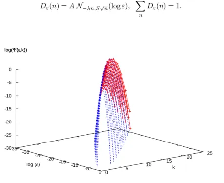
with z = log(ε) fixed, and properly normalized via the constant A to yield the discrete distribution Dε(n)): Dε(n) = A N−λn,S√n(log ε), X n Dε(n) = 1. (49) k log (ε) -30 -25 -20 -15 -10 -5 0 log(Ψ(ε,k)) 0 5 10 15 20 25 -35 -30 -25 -20 -15 -10 -5 0 log(Ψ(ε,k))

Figure 10: Distribution function Ψ(ε, n) (red lines, points) and N (z, n) (blue lines) compared (for definitions, see text), in the case of Fig. 8.

This conjecture is indeed validated numerically in Figure 10, that reports

Dε(n) and Ψ(ε, n) for the same case of Figs. 8, 9. In conclusion, we can write the distribution function p(ε, k) as

p(ε, k) =X

n

Dε(n)p(n, k), (50)

where Dε(n) has mean ¯n = −z/λ and standard deviation s = λ−3/2S

√ −z,

sharply localized in the interval [n − s, n + s]. This explains the shape of the graph reported in Fig. 8, that is to be compared with that of Fig. 1 in Section 3: the Gaussian smoothing is particularly evident near the line k = − log(ε)/λ. Finally, eq. (50) is the basis to derive formulae akin to those of Sect. 3. In particular, it validates the analogue of formula (25) that becomes here:

lim ε→0 log p(ε, −δ log(ε)/λ) log ε = 1 − δ λ H( 1 δ− 1). (51)

The same observations about convergence of the limit detailed in Sect. 3 apply here. One can therefore relate the asymptotic of return time distributions and R´enyi entropies also in the case of expanding maps of the interval.

5

A second approach to expanding maps

In this section, we present a second, more general approach to the statistics of first returns in balls for one-dimensional piecewise linear expanding maps of the type studied in the previous section. This approach can be fruitfully extended to more general situations and, informal as it is now, clearly points to the direction where rigor can be achieved.

Recall the theory of Sect. 3: the word labelling each cylinder of length k was continued periodically to length n to single out a cylinder of length n and return time k. Geometrically, for the kind of maps studied in Sect. 4, each cylinder σ of length k contains a fixed point of the map, xσ, of period k. Balls of radius ε centered at a point x located in the vicinity of such fixed point have a non-empty intersection with their k-th iterate if the distance between x and

xσ is less than _2(ssk_k+1₋₁₎ε, where sk is the derivative of Tk at the fixed point

xσ. Observe that sk grows geometrically as k grows, so that when k is large

sk+1

sk−1 ' 1. In conclusion, all points x in the interval Bε/2(xσ) are such that their

ε-neighborhood returns after time k: Tk_(B

ε(x)) ∩ Bε(x) 6= ∅. Of course, not all of these intervals, labelled by σ, are disjoint among themselves, both with the same and different length of σ. Therefore, two conditions are to be met to assess a genuine first–return.

We may approximately assume that the first condition (non-overlapping of the interval Bε/2(xσ) with other intervals associated with the same period, |σ| =

k), is met when sk+1

sk−1ε is less than the geometrical size, `(Cσ), of the cylinder

that contains the fixed point. More simply, because of our previous observation, we may just require ε < `(Cσ). Let again Σk := {0, . . . , M − 1}k be the set of all words of length k. Within this set we therefore define the subset

Lε,k:= {σ ∈ Σk s.t. ε < `(Cσ)}. (52)

The second condition (non-overlapping of Bε/2(xσ) with intervals with smaller periods |σ|) is more subtle, and can be resolved by considering, among all fixed points xσ of period k, only the primitively periodic ones. We so define the set

Wk:

Wk := {σ ∈ Σk s.t. there is no j < k s.t. σ is periodic of period j}. (53) Summing up, we can write

p(ε, k) = X

σ∈Lε,k∩Wk

µ(Bε(xσ)), (54)

where xσ is the periodic point in the cylinder Cσ. This last expression can be further simplified, using a similar approximation to that employed in Sect.

3. In fact, we can write µ(Bε(xσ)) ' εαµ(xσ), where αµ(xσ) is the local di-mension of the measure µ at xσ. This last quantity can then be extrapo-lated from the measure and the geometric length of the cylinder Cσ: αµ(xσ) ' log(µ(Cσ))/ log(`(Cσ)). As a consequence, eq. (54) becomes:

p(ε, k) = X

σ∈Lε,k∩Wk

εlog(µ(Cσ))/ log(`(Cσ))_{. (55)}

We have compared numerically the function p(ε, k) for the case of Fig. 8 of the previous section and its approximation, eq. (55), in Fig. 11. Agreement is rather satisfactory. -30 -25 -20 -15 -10 -5 0 0 ₅ 10 15 ₂₀ 25 -35 -30 -25 -20 -15 -10 -5 0 -30 -25 -20 -15 -10 -5 0 log p(ε,k) k log ε log p(ε,k)

Figure 11: Distribution function p(ε, k) (green lines) from the original data in Fig. 8 and approximation from formula eq. (55) (red lines)

Eq. (55) can also be written

p(ε, k) = X

σ∈Lε,k∩Wk

µ(Cσ)log(ε)/ log(`(Cσ)). (56)

This last equation is particularly meaningful. Observe first that this generalizes eqs. (21) and following and can be used to the same scope. Secondly, put

λσ := − log(`(Cσ))/|σ|. Then, µ almost surely, when |σ| tends to infinity, λσ converges to the Lyapunov exponent, λ, of the measure µ. Therefore,

p(ε, k) = X

σ∈Lε,k∩Wk

Suppose now to choose ε and |σ| such that −δ log ε = |σ|λ, with 0 < δ < 1. This choice has two effects. First, the exponent in the previous equation becomes 1

δ.

Second, the measure of the set Lε,ktends to one, when ε tends to zero, because

µ almost surely − log(`(Cσ))/|σ| tends to λ, so that almost surely `(Cσ) > ε. Hence, p(ε, −δ log ε λ ) ' X σ∈Wk µ(Cσ) 1 δ. (58)

If we now let k to be a prime number, the set Wk contains all words except the “fixed points” σi = a, for i = 0, . . . , k − 1, where a ∈ {0, . . . , M − 1}. In general, one should also subtract all words of shorter periods that divide k, as done above. Call this set of words Fk. Then,

p(ε, −δ log ε λ ) ' X σ∈Σk µ(Cσ) 1 δ − X σ∈Fk µ(Cσ) 1 δ. (59)

It could be shown that, in systems with sufficiently fast decay of correlations like Bernoulli or Markov, the first term is dominant in the limit, so that discarding the second when taking logarithms and dividing by log ε, one gets

1 log εlog p(ε, − δ log(ε) λ ) = 1 log εlog( X σ∈Σk µ(Cσ) 1 δ) = δ λ 1 klog( X σ∈Σk µ(Cσ) 1 δ). (60) Taking the limit, we obtain a new verification of eq. (51)

lim ε→0 1 log εlog p(ε, − δ log(ε) λ ) = (1 − δ) λ H( 1 δ− 1). (61)

In the next section, we shall see a generalization of this equation.

6

Linear automorphisms of the two-dimensional

torus

The general framework presented in the last section can be easily extended to treat the case of linear automorphisms of the two-dimensional torus, of which the Arnol’d cat map is the most celebrated example. For convenience, we choose a metric in the torus such that balls of radius ε are euclidean squares of side 2ε with sides oriented along the stable and unstable directions and for simplicity we consider the case when these directions are orthogonal. Then, one can easily show that around any fixed point of the k-th iteration of the map there exists a rectangle, with sides oriented in the stable and unstable directions, of points

x whose ε-balls intersect their image after k iterations. Letting λ− and λ+ the

(increasingly ordered) eigenvalues of T , the sides of this rectangle have length

ε(1+ 2λk−

λk

−−1) and ε(1+

2

λk

+−1). As it turns out, for the Arnol’d cat and other

of initial conditions just described is a square. Figure 12 draws these squares at a fixed value of ε.

We can then repeat a two-dimensional generalization of the arguments of the previous section. This we will do elsewhere, but we will provide the result below. In fact, an even simpler argument can be sketched. We have seen above that a square of area ε2_{(1 +} 2

λk

+−1)

2 _{exists at each fixed point of T}k _{and is} characterized by return times k, or less. This area quickly becomes ε2_{to a good}

approximation. Moreover, the number of periodic points of Tk _{grows like λ}k

+.

Then, when ε is “small” with respect to k, neglecting all other considerations, we can write

p(ε, k) ' ε2_λk

+. (62)

Of course, we have to make precise what we mean by “small”. This is when

ε2_λk

+ ≤ 1. Equality holds for kε = −log(λ2 log ε+). Indeed, following the results

reported in Sect. 2, 2

log(λ+) is the almost sure limit of

τ (Bε(x))

− log ε , since it coincides

with 1

log(λ+) − 1

log(λ−), see eq. (12). Moreover, in this case D1(µ) = 2, the

invariant measure being the Lebesgue measure and the entropy hµ is equal to the Lyapunov exponent λ = log(λ+). Figure 13 draws the distribution function

p(ε, k) for a different toral automorphism, just chosen to increase variety: that

associated with the matrix (1, 2; 2, 5). The logarithmically flat approximation in eq. (62) fits the data almost perfectly in the region ε2_λk

+≤ 1.

If we now turn our consideration to the line k = δkε in the (k, log ε) plane, with 0 < δ ≤ 1, we can prove that the quantity p(ε, δkε) verifies in this two-dimensional case the analogue of eq. (26):

lim ε→0 1 log εlog p(ε, − δ log(ε) λ/2 ) = (1 − δ) λ/2 H( 1 δ− 1). (63)

The detailed proof, obtained along the lines of Sect. 5 will be reported elsewhere. We simply compute here the two sides of the equality (63), showing that they are equal. From eq. (62) we can compute the l.h.s., obtaining

lim ε→0 1 log εlog p(ε, − δ log(ε) λ/2 ) = 2(1 − δ). (64)

On the other hand, the R´enyi entropies for the Lebesgue measure and the Arnol’d cat dynamics are all equal to λ = log(λ+), so that also the l.h.s. of

eq. (63) is equal to 2(1 − δ).

We conclude this section by taking inspiration from eq. (63) to put forward a conjecture: we believe that, letting η be the almost sure limit of τ (Bε(x))

− log ε ,

see eq. (10), and letting kε= −η log ε as before, under sufficient hypotheses of mixing, one has

lim ε→0 1 log εlog p(ε, δkε) = (1 − δ) η H( 1 δ − 1). (65)

0 0.1 0.2 0.3 0.4 0.5 0.6 0.7 0.8 0.9 1 0 0.1 0.2 0.3 0.4 0.5 0.6 0.7 0.8 0.9 1

Figure 12: Initial conditions x in the two-dimensional torus color coded accord-ing to the return time of the ball Bε(x) of radius ε = 0.15 for the Arnol’d cat map. (τ = 1 red, 2 green, 3 blue, 4 magenta, 5 light blue)

7

Conclusions

We have studied in this paper various aspects of the statistics of return times of sets in dynamical systems.

We have first reviewed known results for symbolic ψ-mixing systems, that link return times and R´enyi entropies. We have established new “counting rules”, embodied in the sets Wn,k and in the lemma of eq. (28) that have per-mitted us to explain the slow convergence of the quantities studied in previous works. At the same time, these results have lead to the definition of a new “partition function” Zp(δ, n), eq. (33), that best achieves the goal of extracting R´enyi entropies from return times statistics.

When considering return times for balls, we have established a general re-lation holding for one-dimensional expanding maps, eq. (51), that links the asymptotic of return times with R´enyi entropies and the Lyapunov exponent. This relation has been obtained developing two different approaches. The former is a quantitative comparison between balls and dynamical cylinders especially developed for this case. The second is a more general argument that well de-scribes the full behavior of the statistics p(ε, k), comprised in eq. (55).

We have finally considered linear automorphisms of the two dimensional torus, like the Arnol’d cat map, for which a “quick and dirty” analysis is capable of describing the correct behavior of the distribution function p(ε, k). This has

-12 -10 -8 -6 -4 -2 0 0 2 4 6 8 10 12 14 16 18 -16-14 -12-10 -8-6 -4-2 -12 -10 -8 -6 -4 -2 0 log(p(ε,k)) k log(ε) log(p(ε,k))

Figure 13: Distribution function p(ε, k) for the toral automorphism associated with the matrix (1, 2; 2, 5).

permitted us to write the formula in eq. (63) that links return times statistics and R´enyi entropies with η, the almost-sure value of the limit in eq. (10). This formula is an extension of that obtained for one-dimensional systems and we have conjectured that it should hold in much more general situations than the one presented in this paper.

As stated in the Introduction, the character of this paper is tailored to the audience expected for this volume, that comprises both specialists in dynamical systems and in other disciplines. We have therefore tried to present our results in the most transparent form, while renouncing at times to full rigor in favor of clarity. We are nonetheless convinced that most of the theory developed here touches upon new ideas and approaches, and presents more than valuable hints to where a rigorous treatment will be developed, as we plan to do in forecoming publications.

References

[1] M Abadi, Sharp error terms and necessary conditions for exponential hit-ting times in mixing processes, Ann. Probab., 32 (2004), 243–264.

[2] M Abadi, Hitting, returning and the short correlation function, Bull. Braz.

[3] M Abadi and A Galves, Inequalities for the occurrence times of rare events in mixing processes. The state of the art, Markov Proc. Relat. Fields., 7 (2001), 97–112.

[4] M Abadi and S Vaienti: Large Deviations for Short Recurrence; Disc. Cont.

Dyn. Syst. 21 729–747 (2008).

[5] V Afraimovich, Pesin’s dimension for Poincar´e recurrence, Chaos 7, 11-20, (1997).

[6] V Afraimovich, J-R Chazottes and B Saussol, Pointwise dimensions for Poincar recurrence associated with maps and special flows, Disc. Cont.

Dyn. Syst., 9 (2003), 263–280.

[7] V Afraimovich, E Ugalde and J Urias, “Fractal Dimensions for Poincar´e Re-currence”, Monograph Series on Nonlinear Sciences and Complexity, Vol. 2, Elsevier, (2006)

[8] L Barreira, Ya Pesin, J Schmeling, On a General Concept of Multifractality: Multifractal Spectra for Dimensions, Entropies and Lyapunov Exponents,

Chaos, 7:1, 27-38, (1997)

[9] C Beck and F Schl¨ogl, “Thermodynamics of Chaotic Systems”, Cambridge University Press, 1993.

[10] D Bessis, G Paladin, G Turchetti and S Vaienti, Generalized dimensions, entropies and Lyapunov exponents from the pressure function for strange sets, J. Stat. Phys., 51 (1988), 109–134.

[11] C Bonanno, S Galatolo and S Isola, Recurrence and algorithmic informa-tion, Nonlinearity, 17 (2004), 1057–1074.

[12] P Collet, A Galves, B Schmitt, Fluctuations of repetition times for Gibbsian sources, Nonlinearity, 12, 1225-1237, (1999)

[13] A Csordas and P Szepfalusy, Generalized entropy decay rate of one-dimensional maps, Phys. Rev. A, 38 (1989), 2582–2587.

[14] J-P Eckmann and D Ruelle, Ergodic theory of chaos and strange attractors,

Rev. Mod. Phys., 57 (1985), 617–656.

[15] P Ferrero, N Haydn and S Vaienti, Entropy fluctuations for parabolic maps,

Nonlinearity, 16, (2003), 1203–1218

[16] A Galves and B Schmitt, Inequalities for hitting times in mixing dynamical systems, Random Comput. Dyn., 5 (1997), 337–348.

[17] P Grassberger and I Procaccia, Estimation of the Kolmogorov entropy from a chaotic signal, Phys. Rev. A, 28, 2591–2593, (1983)

[18] P Grassberger and I Procaccia, Dimensions and entropies of strange at-tractors from a fluctuating dynamics approach, Phys. D, 13 (1984), 34–54. [19] N Haydn, Y Lacroix and S Vaienti: Hitting and Return Times in Ergodic

Dynamical Systems: Ann. of Probab. 33 (2005), 2043–2050

[20] N Haydn and S Vaienti, The limiting distribution and error terms for return time of dynamical systems, Disc. Cont. Dyn. Syst., 10 (2004), 584–616. [21] N Haydn, S Vaienti, The R´enyi Entropy Function and the Large Deviation

of Short Return Times, accepted for publication in Ergodic Theory and Dynamical Systems

[22] M Hirata, B Saussol and S Vaienti, Statistics of return times: a general framework and new applications, Comm. Math. Phys., 206 (1999), 33–55. [23] D Ornstein, B Weiss, Entropy and data compression schemes, IEEE Trans.

Inf. Theory, 39 (1993) 78-83.

[24] G Paladin, G Parisi and A Vulpiani, Intermittency in chaotic systems and R´enyi entropies, J. Phys. A, 19 (1986), L997–L1001.

[25] V Penn´e, B Saussol and S Vaienti, Dimensions for recurrence times: topo-logical and dynamical properties, Disc. Cont. Dyn. Syst., 5 (1999), 783– 798.

[26] Ya Pesin, “Dimension Theory in Dynamical Systems”, University of Chicago Press, (1997)

[27] A R´enyi, “Probability Theory”, North Holland, Amsterdam, (1970) [28] S Robin, F Rodolphe, S Schbath, ”DNA, Words and Models”, Cambridge

University Press, (2005)

[29] B Saussol, S Troubetzkoy and S Vaienti, Recurrence, dimensions and Lya-punov exponents, J. Stat. Phys., 106 (2002), 623–634.

[30] B. Saussol, S. Troubetzkoy, S. Vaienti, Recurrence and Lyapunov expo-nents, Moscow Math. Journ., 3, (2003), 189-203

[31] F Takens and E Verbitsky: Generalized entropies: R´enyi and correlation integral approach, Nonlinearity, 11 (1998), no. 4, 771–782

[32] F Takens and E Verbitsky: Multifractal analysis of local entropies for expansive homeomorphisms with specification, Comm. Math. Phys., 203, 593–612, (1999)