HAL Id: tel-00737746
https://tel.archives-ouvertes.fr/tel-00737746v2
Submitted on 18 Oct 2012HAL is a multi-disciplinary open access
archive for the deposit and dissemination of sci-entific research documents, whether they are pub-lished or not. The documents may come from teaching and research institutions in France or abroad, or from public or private research centers.
L’archive ouverte pluridisciplinaire HAL, est destinée au dépôt et à la diffusion de documents scientifiques de niveau recherche, publiés ou non, émanant des établissements d’enseignement et de recherche français ou étrangers, des laboratoires publics ou privés.
How large spheres spin and move in turbulent flows
Robert Zimmermann
To cite this version:
Robert Zimmermann. How large spheres spin and move in turbulent flows. Other [cond-mat.other]. Ecole normale supérieure de lyon - ENS LYON, 2012. English. �NNT : 2012ENSL0730�. �tel-00737746v2�
Thèse
en vue de l’obtention du grade de
Docteur
de l’École Normale Supérieure de Lyon – Université de Lyon
Laboratoire de Physique &
Ecole Doctorale de Physique et Astrophysique
How Large Spheres spin and move
in Turbulent Flows
−4 −2 0 2 4 5 6 7 8 9 10 11 12 13 B T Ne
q
présentée et soutenue publiquement le 13 juillet 2012
par
Robert ZIMMERMANN
sous la direction de
Romain VOLK et Jean-François PINTON
après l’avis de
Haitao XU et Alex LIBERZON
devant la commission d’examen formée de
Christophe BAUDET Examinateur
Luminita DANAILA Examinateur
Alex LIBERZON Rapporteur
Jean-François PINTON Directeur de thèse
Romain VOLK Co-directeur de thèse
obert immermann
abriqué en rance
Contents
1 Introduction
2 A very intermittent introduction to turbulence
luid dynamics cales
uler agrange the motion of particles
on ármán swirling ows
n estimating ow parameters
3 Setup, Technique & Measurements
xperimental etup
on ármán ow
articles
mage acquisition processing
osition racking
rientation racking
ath
racking
obustness
fficiency further development
ata runs
4 How they move
otion
s
utocorrelations
iscosity density
ampling
5 How they spin
otational dynamics
ngular velocity acceleration
nergy
oupling between rotation translation
renet frame
n uence on the centrifugal force
6 How they fluctuate
inetic nergy
istribution of εva
ime scales
stepbystep test of the uctuation theorem
πτ lter and their implications on agrangian data
hape of πτ ummary
7 An instrumented particle measuring Lagrangian acceleration
n instrumented particle
esign echnical etails
alibration esolution
rientation of the sensor within the capsule
uns
irectly accessible quantities
hakiness
oments of atrans
n uence of inertia imbalance
utocorrelations
ime scales
stimating ow parameters
nergy transfer rate
imultaneous racking cquisition
greement between tracking acceleration signal
ontribution of the different forces
utocorrelations
uantities accessible only to the tracking
ummary deas
8 Conclusion A Sidetracks
he second agrangian xploration module
ixing in chemical reaction rst results of a fast local and continuously operating pprobe
irst easurements
B Appendix
nwrapping ifferences
ngular elocity cceleration
utocorrelations tructurefunctions
renet formulas
exture
itting an ellipsoid
Remerciements
he dissertation you are holding in your hands is the fruit of a bit more than three years at the cole ormale upérieure de yon and am deeply grateful for the help support and presence of many folks who made this time not only instructive and productive but also fun – merci beaucoup!
n premier lieu je voudrais remercier eanrançois inton pour sa con ance son ent housiasme contagieux et en général pour la grande latitude et souplesse de travail quil ma accordé pendant ma thèse e tiens également à remercier beaucoup omain olk pour le suivi et laide en salle de manip et le combat perpétuel contre les mystères insondables de ladministration française
e remercie tout le labo de physique pour son accueil son aide et sa tolérance envers mon français jimagine que cétait dur – surtout au début e suis en particulier heureux que icolas ophie elphine anny athanaël inshan ickaël lain ichel oann et ionel aient pris part à cette thèse n plus davoir partagé leur bureau les manips et du bon temps en dehors du labo ces deux derniers mont aussi initié à la culture française1
e remercie la ville de yon pour avoir organisé un feu darti ce le soir de ma soutenance
d like to thank the members of the committee for their work in refereeing my disser tation
in großer ank geht auch an meine amilie und an meine mi die mit über an ng ranzösisch zu lernen
ercithanksgraciasteşekkürlerdziękujędanke for this awesome time to he crazy chemists llie acek enaf aja ichel die inguine va und uillaume drian osia ulia risti urkel odo rederine werg ase reg hloé the rasmus folks athieu du erthom le qui a nancé notre séminaire de bière the climbing hall
nd of course teşekkürler mel for everything öptüm
1entre autres les s les sketchs des nconnus les lapins crétins hapi hapo éléchat et la cité de la
1 Introduction
ature is full of ows and many of them are turbulent and transport objects n nature one encounters such particleladen ows for example as rain droplets in a thundercloud transport of pollen and seeds with the wind or of sediments in a river hey play an important role in industrial applications too e it the atomizing of gasoline in a motor sewage treatment chemical mixers or weather balloons
he turbulent motion of ows itself is a yet unsolved problem characterized by its high irregularity and its uctuations in both time and space oreover turbulence covers a large range of scales nergy is injected at large scales where it drives the creation of large eddies which continuously break up into new eddies he whirls interact and disperse until they reach a size where viscosity plays a role and their kinetic energy is dissipated into heat articles immersed in such a ow are consequently subject to a complicated interaction with eddies of all sizes
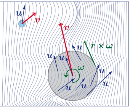
ince the time of uler avier and tokes huge progress has been made in understanding the motion of spherical particles of size D much smaller than the smallest length scale of the ow the olmogorov scale η ecause of the small size of the particle the ow around it is locally laminar – see ig – therefore the equation governing the particle velocity v can be determined by solving the uid equations once the uid velocity u is known n the simplest case the particles are subject to the tokes drag and the added mass term thus the velocity v can be determined by solving a simple differential equation or D → 0 the velocity of a neutrally buoyant particle reduces to the uid velocity u so the particle behaves as a uid tracer his property is crucial for several experimental techniques
ith the advent of agrangian measurement techniques material particles are gaining attention hese particles have a size larger than η but are still small compared to the largest scales in the ow s suggested by ig their case is conceptually much more difficult
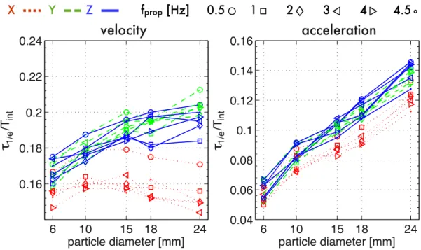
y studying the acceleration statistics of a particle one can infer on the dynamics of the forces acting on it xperiments have shown that upon increasing the ratio D/η from 1 to 40 the variance of the particle acceleration i.e. of the forces decreases as (D/η)−2/3
evertheless the uctuations of force remain non–gaussian up to D/η ≲ 40
ince material particles decrease their acceleration variance with increasing size they share common properties with heavy inertial particles for which the behavior is well determined by their size ratio D/η till large neutrallybuoyant particles cluster differently than inertial particles t present a full derivation of the equation of motion of a large particle is still not available
parable to the large scales is surprisingly little studied his is partially due to the fact the description of a solid object freely advected in a uid requires in addition to its transla tional degrees of freedom characterizing its position three rotational degrees of freedom specifying its orientation with respect to a reference frame he evolution of its position and of its orientation depends according to ewtons laws on the forces and torque act ing on the particle at each instant which result from the interaction between the object and the turbulent ow
n the preceding work of oann asteuil it was observed that a neutrally buoyant sphere of a size D ∼ 0.6 Lint i.e. comparable to the large scales of the ow is highly
intermittent in both translation and rotation imulations at low turbulence levels show that particles of D/Lint ∼ 1 alter the surrounding ow up to a distance of twice their
diameter ecently this has been supported by imon lein athieu ibert and others who simultaneously followed tracer particles and rigid gel spheres in a highly turbulent environment
Figure 1.1:ketch of a small and a large particle superimposed on local stream lines hereas the ow around the small particle is smooth it exhibits signi cant spatial varia tions around the large particle
he present experimental study investigates the motion of neutrally buoyant spheres whose diameter D is of the order of the integral scale Lint n addition we aim at resolving the
six degrees of freedom of the particle dynamics herefore we developed a novel mea surement technique which enables us to obtain a simultaneous tracking in time of the particles position and its absolute orientation with respect to a reference frame
revious studies focused on directly measuring the angular velocity without resolving the absolute orientation as a function of time e and oco tracked dots painted
on a particle with high speed cameras and computed the angular velocity from their dis placement between two consecutive frames ecently lein et al. adapted a particle tracking system to this approach luorescent tracer particles sticked to the surface of transparent gel spheres and tracer particles suspended in the carrier ow are tracked in space the spheres rotation is then given by the relative displacement of the sticked parti cles owever identifying which are attached to a moving spheres surface and which are moving freely with respect to the others is a nontrivial task completely different ansatz was taken by rish and ebb who created an ulerian technique measuring one component of the angular velocity using specially engineered transparent particles which contain an embedded mirror he reported particle diameter is less than µm which is of the order of the olmogorov length scale η ur approach is completely different it consists in painting the particle with a suitable layout and in retrieving its orientation or algorithmic efficiency and robustness this is not done step by step but for the entire trajectory using a global path extraction he experimental setup and the technique are presented in chapter
aving access to particles translation and rotation enables us to study the forces and torques acting on a large inertial particle thus permitting to ask yet fundamental ques tions about their dynamics ore speci cally three questions are addressed irst general features of the translation are presented in chapter ext we turn to the rotation of a solid large particle chapter and show that despite the highly turbulent ow rotation and translation couple according to the lift force Flift = Cliftvrel × ω istorically a
coupling between the rotation and translation was rst reported by agnus in in his article Über die Abweichung der Geschosse, und: Über eine auffallende Erscheinung bei rotierenden Körpern1 and a lift has been measured in laboratory experiments when the ow is steady and laminar t has further been observed for stationary objects in a rotating ows but to our knowledge we report here the rst observation of a lift force for a freely moving sphere in a turbulent ow n the third part chapter we test how the particle exchanges momentum with the uid or that purpose we analyze the uctuations of the particles kinetic energy by means of the uctuation theorem urthermore in collaboration with mart a young startup on the campus and building upon the work of oann asteuil et al. we present a novel measurement apparatus for characterizing ows in chapter n instrumented particle which contin uously transmits its threedimensional agrangian acceleration he particle embarks a small battery a accelerometer operating at 316 z and a wireless transmission system its signal is then received and processed on a control computer fter a general presen tation of the apparatus the developed methods for the interpretation of the acceleration signal are explained e further test its precision by tracking the position and orientation of the particle while simultaneously recording its acceleration signal
ome parts explored during the ½ years of this thesis do not fully t within the storyline of the manuscript hese sidetracks are therefore presented separately in appendix
2 A very intermittent introduction to
turbulence
his chapter recalls some features and concepts of turbulence and the tools used n a way its as intermittent as our particles motion slower and less intermittent introduction can be found in the following books
ope Turbulent Flows audau and ifschitz Hydrodynamics achelor an intro-duction to uid dynamics risch Turbulence: e Legacy of A. N. Kolmogorov and in ennekes and umley A First Course in Turbulence comprehensive source of information on the various experimental techniques which were developed in uid dynamics research is found in the Springer Handbook of Experimental Fluid Dynamics
2.1 Fluid dynamics & Scales
t some point during ones study of physics or engineering one learns that the motion of a uid is govern by the aviertokes equation n most cases this is restricted to incompressible uid of constant viscosity ν and constant uid density ρf
[ ∂ ∂t+ u∇ ] u =−∇p ρf + ν∇2u + 1 ρf f
where u is the velocity eld p the pressure and f external forces per body volume n addition the uid is subject to the continuum equation ∇ u = 0 and the boundary conditions he term (u ∇) u is quadratic and only for some special cases one can nd analytical solutions ost of those fall into the regime when viscous forces dominate – i.e. ν∇2u > (u∇) u – and one therefore introduces the socalled Reynolds number
as a dimensionless parameter relating the inertial and viscous term
Re = agnitude [(u ∇) u] agnitude [ν∇2u] =
U L
ν
where L and U represent the characteristic length and velocity scale of the ow one can interpret the eynolds number as an indicator of the level of turbulence or Re≪ 1 the viscous term dominates and small perturbations arising from the boundaries or body forces acting on the uid are damped out he ow is then organized in stationary streamlines ne can picture its structure as uid lamina which glide along each other but do not cross ence this type of ow is called laminar
or an increasing eynolds number perturbations arising from the boundaries or body forces acting on the uid are not damped out anymore and the lamina break up into
Re=26
Re=0.16 Re=2 000
Re=10 000
Figure 2.1:low behind a cylinder at different eynolds numbers xtract from the album of uid motion t very low eynolds number Re = 0.16 the ow is organized in streamlines passing smoothly around the cylinder a socalled creeping or tokes ow but with increasing eynolds number more and more eddies of different sizes appear in the ow
many eddies which are advected with the mean ow he system evolves into a spatio temporal chaotic system which is called turbulence n this regime mixing is enhanced but also the drag force acting on a body moving through the ow is higher in a turbulent ow than in the laminar case o illustrate this transition ig shows extracts from the album of uid motion for the ow around a cylinder at four different eynolds numbers t Re = 0.16 the ow is organized in streamlines passing smoothly around the object this con guration is also called a creeping or tokes ow ut with increasing eynolds number more structures of different sizes appear in ow heir interaction yields the complex multiscale nature in both time and space of fully turbulent ows ne therefore turns towards a statistical description of turbulent ows
Richardson cascade ichardson formulated the multiscale nature of turbulence in his famous poem
Big whorls have little whorls that feed on their velocity, and little whorls have smaller whorls and so on to viscosity.
n olmogorov published groundbreaking articles translating this idea into math ematical language nergy is injected at a length scale Lint characterizing the biggest ed
dies hese eddies break up into smaller eddies which again break up into even smaller whirls he cascade stops when viscosity becomes nonnegligible and injected energy is
Inertial Range
Energy injection
Range
Dissipative
Range
L
appL
intλ
η
τ
ηT
intFigure 2.2:ketch of the ichardson cascade he system of size Lapp injects energy at
the size Lint characterizing the biggest whirls hese whirls break up into smaller whirls
which break up into even smaller eddies and so forth his process is stopping in the dissipative range when viscosity becomes nonnegligible and the injected energy is nally converted to heat his model does not describe the dynamics of the eddies
converted into heat nergy conservation dictates that the energy injected at large scales must be the energy dissipated at the small scales ne therefore de nes the energy trans fer rate1ε as the injected power per mass unit imensional arguments relate the energy transfer rate to the velocity ulof an eddy of length l
εl ∼ u3
l
l
olmogorov then assumes that far away from the energy injection scales the eddies lost their memory of their creation f dissipation is still negligible then the statistics are fully determined by ε this is the socalled inertial range he end of the cascade is referred to as dissipative range which is fully characterized by viscosity ν and energy injection rate ε hen the smallest characteristic length scale η and time scale τη of the ow are
η =(ν3/ε)1/4 a
τη = (ν/ε)
1/2
b ne generally speaks of η and τηas olmogorov scales ne can further deriveidentify an
intermediate scale situated between the largest and the smallest eddies he aylor micro scale λ and it is common to specify the turbulence level at this scale by the eynolds
number based on the aylor micro scale Rλ ≈ √
15 Re ne can further relate the olmogorov scales to the biggest or integral scales of the ow
η/Lint ∝ Re−3/4 a
τη/Tint ∝ Re−1/2 b
where Tintis the time scale of the large eddies of the ow consequence of the equations
is that the olmogorov scales and the biggest scales of the ow become more sepa rated with increasing Re his conclusion is sometimes referred to as Kolmogorov’s idea of scale separation n illustration of the cascade is provided in ig ll measurements presented within this manuscript consider particles whose diameter is a fraction of the integral length scale and much larger than the olmogorov scale
ne should keep in mind that the ichardson cascade does not describe the dynamics within the cascade imilarly olmogorovs derivations assume that the turbulent uctu ations are locally homogeneous and isotropic stablishing such conditions in the lab is a demanding task and outside a research facility they are almost never encountered ore over lum et al. showed for a variety of turbulence creating apparatuses and eynolds numbers that a signature of the large scales can still be found in the small scales
2.2 Euler, Lagrange & the motion of particles
There are some things in life which are more fun doing than watching
(Jean-François Pinton)
s for many things there are at least two perspectives one can either observe at xed position without participating in the uids motion or one can be advected by the ow and describe the local interaction along ones trajectory through the ow he descriptions are the socalled Eulerian and Lagrangian frame athematically the ulerian frame works with spatiotemporal elds of either vector quantities like the uid velocity u(x, t) or scalars ϕ(x, t) e.g. the temperature n contrast thereto the agrangian frame measures a vector or scalar quantity along a trajectory Y (t)
he two perspectives yield a different view on the dynamics but in the limit of in nite resolution or an in nite amount of trajectories through the ow eld both expressions can be converted into the other he agrangian frame is the natural choice when describing the motion of objects advected in the ow
ormally one choses the description which is suitable for the problem asked omplex problems necessitate information from both sides e.g. to predict the spread of volcano ash it is important to ask how do dust particles usually behave as well as how is the wind today
Figure 2.3:moke visualization of the ow around a baseball spinning at 630 rpm in a windtunnel at 23.5 m/s xtract from the album of uid motion ote the turbu lent wake which extends over several particle diameters he streamlines are bent down wards due to the rotation of the sphere
Particles bjects in ows come in many shapes e focus here on homogeneous rigid spheres which are characterized by their diameter Dpart and their density ρp he in u
ence of their surface roughness is neglected n order to compare different experiments one usually takes the ratio of the diameter to the biggest Dpart/Lint or smallest Dpart/η
length scale and of the particles density to that of the uid
β≡ 3 ρf 2 ρp+ ρf
ll data presented in this manuscript is gained with neutrally buoyant particles – i.e. ρp = ρf β = 1
fter de ning these parameters one can ask what happens if a particle is inserted into a ow ig shows a visualization of the ow around a spinning baseball one sees how the stream lines are bent by the particle he wake is clearly turbulent and extends over several particle diameters oreover one observes the in uence of the rotation on the streamlines derivation of the equation of motion for such a realworld example is an extremely complex problem
n the case of small particles one can assume that the ow is modi ed only locally evertheless one has to take care of the noslip condition the uid velocity matches the particle velocity at the surface priori the particle can and does rotate hence the noslip condition induces the forces and torques acting on the particle n order to characterize the ow on the scale of the particle one de nes a eynolds number based on the particle
Rep =
Dpart vslip
ν
where the slip velocity vslip is the velocity difference between particle and surrounding
ow
he equation of motion for a small particle with a small particle eynolds number has been derived by axey and iley and independently by atignol
ρp d dtvpart= ρf [ ∂ ∂t + u∇ ] u Y (t) | {z } pressure gradient + (ρp− ρf) g | {z } buoyancy force −ρf 2 d dt ( vslip− a2 10∇ 2u Y (t) ) | {z } added mass − 9νρf 2a2 ( vslip−a 2 6 ∇ 2u Y (t) ) | {z } viscous drag − CLρfvslip× ωp | {z } lift force − 9ρf 2a √ ν π ∫ t 0 (t− τ)−12 d dτ ( vslip(τ )− a2 6∇ 2 u Y (t) ) dτ | {z } history force 20
t is u the ow eld in absence of the particle a = Dpart/2the particle radius Y (t) the
particle position and vpartits velocity vslip = vpart(t)−u [Y (t), t] is the velocity difference
between particle and unaltered ow u at the particle position Y (t) ∇2u
Y (t) stems
from the axén corrections which take into account the nonuniformity at the scale of the particle of the ow hey vanish in a locally uniform ow eld
he different terms tell of the various forces acting on the sphere buoyancy and pressure are the direct uidmechanical counterpart of ewton mechanics s the particle moves through the ow is has to accelerate its surrounding uid and thus loses momentum his effect appears as an added mass ince the ow is homogeneous at the scale of the particle the classical tokes force is an adequate description of the viscous drag he wake of the particle acts back on the particle and has some memory of its motion his is accounted for with the history force term ince its calculation is extremely demanding this term is very often omitted n the case of a creeping or tokes ow Rep ≪ 1 around the
particle rotation and translation decouple and there is no backreaction from the torque on the particle velocity n this case it is furthermore possible to reduce equation to the tokes drag and the added mass term he inertiadensity of the particle is then represented by the time scale τp in which it reacts to changes in the ow and the so
called Stokes number becomes the sole nondimensional parameter relating the particles inertia to the smallest time scale of the ow
St≡ τp τη = D 2 part 12 ν β 1 τη = 1 12β ( Dpart η )2 t should be stressed that this simpli cation is limited to small particles Dpart ≲ η
or higher Rep a rotating particle experiences a lift or agnus force his nonlinear
and invsicid contribution couples rotation and translation of the particle he term is not part of the original axeyiley equation t was added later by uton e discuss it and the rotation of larger particle in more detail at the beginning of chapter enée atignol further derived the torques acting on a particle
d dt(Jωp) = T =− 8πρf ν a 3(ω p − ωf/2) | {z } drag torque + 8 15π a 5ρ f [ ∂ ∂t+ u∇ ] ωf | {z } uid vorticity −8πρfν a3 3 ∫ t 0 d (ωp− ωf/2) dτ exp ( ν (t− τ) a2 ) erf √ ν (t− τ) a2 dτ | {z } history torque −8πρfa4 3 √ ν π ∫ t 0 (t− τ)−12 d (ωp− ωf/2) dτ dτ | {z } history torque t is ωp and ωf the angular velocity of the particle and the uid i.e. the vorticity J is
by drag torque and the two history terms and it is driven by the angular acceleration of the underlying ow he torque does not have an equivalent of the added mass term in q n most conditions all terms except the rst are neglected and one obtains
T =−8πρfν a3(ωp− ωf/2)
or a solid homogeneous sphere one can then compute the response time to a torque
τprot = |J| 8πρfν a3
= a
2
15ν
gain this is only meaningful for small particles
articles much larger than the olmogorov scale are not governed by these equations nfortunately no equation exists yet for the motion of large particles oreover direct numerical simulations of the aviertokes equation which take into account the bound ary conditions of a moving object are computationwise extremely expensive n urore aso published work on a xed particle in a turbulent ow at Rλ = 20 for
comparison the turbulence in a cup of coffee has Rλ ≈ 100
2.3 Von Kármán swirling flows
Co–rotation
Counter–rotation
Figure 2.4:low structure in a von ármán ow with co and counterrotating impellers image adapted from ote that the impellers are housed in a square vessel through out this thesis
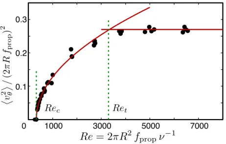
he von ármán swirling ow is a tank with two opposing propellers that create an axisymmetric ow eld he propellers2 can be either co or counterrotating leading to different ow con gurations lades on the impellers work similar to a centrifugal pump and add a poloïdal circulation at each propeller n the counterrotating case the ow is highly turbulent and within a small region in the center the mean ow is little and the local characteristics approximate homogeneous turbulence owever at a large scale it is known to have a large scale anisotropy n extensive characterization can be found in the thesis of lorent avelet e showed that with increas ing propeller speed the ow undergoes a transition through several chaotic states until it reaches a fully developed turbulent state which is characterized by the fact that the uc tuations in velocity grow linearly with the propeller speed n other words the ow is fully turbulent if (v(fprop)
)
/fprop = const. ccording to and as illustrated
in ig the transition to fully developed turbulence occurs at a eynolds number of Ret = 2πR2fprop/ν ≈ 3500 in this dissertation all experiments were performed at
Re > 4000 ence the ow was always fully turbulent
he high turbulence level and con ned ow in an apparatus that ts on a lab bench makes this apparatus highly appealing for agrangian measurements the von ármán ow
0 1000 3000 5000 7000 0.1
0.2 0.3
Figure 2.5:ransition to fully developed turbulence in a cylindrical von ármán ow gure adapted from ote that the eynolds number Re is here simply based on the propeller radius R and the propeller speed fprop Retmarks the transition to fully
developed turbulence ll measurements presented in this thesis have Re > 4000 ence the ow is fully turbulent
became a standard tool for turbulence research ome people even refer to it as the workhorse of turbulence and also the rench washing machine3
n the other hand corotating impellers create a ow similar to a hurricane lose to the axis of rotation the ow is weak followed by a strong toroidal component and an additional poloidal circulation induced by blades on the impellers t the same propeller speed a corotating driving creates less turbulence than counterrotating impellers but the ow is still highly turbulent atherine imand has examined the properties of co rotating von ármán ow in detail during her thesis ithin this manuscript corotating driving is used as a crosscheck but the focus lies on counterrotating impellers
visualization of the ow structures is provided in ig
lthough most experiments reported in the literature are carried out in a cylinder the von ármán ow of this thesis has a container built with transparent at side walls hus the cross section of the vessel is square his rectangular design enables us to perform direct optical measurements over almost the whole ow domain t also reduces a solid body rotation a comparable effect can be achieved by adding baffles to a cylinder he impellers are tted with straight blades such that we observe the characteristic poloidal circulation due to the pumping ore details on the apparatus are found in section
3his is an urban legend the rench have the same washing machines as everybody else
2.3.1 On estimating flow parameters
hen estimating the motion based on general parameters of the ow one has the choice between olmogorov and large scale apparatus type arguments s explained earlier the former evaluates ow parameters e.g. the olmogorov scales ητη in the dissipative and
inertial range based on energy injection rate ε and viscosity ν he derivation assumes that the ow behaves locally homogeneous and isotropic in a statistical sense
hen investigating large particles with a size Dpart comparable to the integral length
scale Lint moving through the whole mixer these assumptions are most likely no longer
valid imilar to the thesis and articles by avelet one can then focus on di mensional arguments which stem from the apparatus hese are in our case the propeller speed fprop the particle diameter Dpartand the radius of the propeller R lthough these
two choices are different in their physical background they yield similar dimensional pre dictions hat is due to scaling relations of fully developed turbulence like ε∝ f3
propand
(v)∝ fprop or a clear distinction we differentiate between the terms
3 Setup, Technique & Measurements
ince ewton it is known that the motion of an object is determined by the forces and torques acting on it ts interaction with the various whirls in a ow results in a complex translation and rotation of the latter or simplicity we limit our investigation to material spherical particles yet we do not restrict their mass distributionver the last years a set of measurement techniques has become available to extract a particles velocity and acceleration and yielded important information on the interactions with the ow or a detailed survey on these techniques the reader is referred to the Handbook of Experimental Fluid Dynamics
aser or coustic oppler elocimetry have direct access to the velocity nfortunately they cannot be extended to measure the rotation and are therefore not further discussed here article racking elocimetry on the other hand follows the particles po sition by means of multiple high speed cameras elocity and acceleration are then the derivatives of the position timeseries urthermore this technique is able to track several particles simultaneously which enables the study of multiparticle statistics like how fast they spread
he rotational component of the particles motion can be obtained by tracking the dis placement of dots on the spheres surface his was rst introduced by e and oco unfortunately a h student had to identify all dots by hand t was recently picked up by athieu ibert imon lein et al. who use a system to track uorescent particles which are attached to large transparent gel spheres dding tracer particles to the ow allows him to directly access the ow of the uid around the spheres n addition no
student is forced anymore to identify the dots by hand owever identifying which trac ers are attached to a moving spheres surface and which are moving freely is a nontrivial task
rish and ebb demonstrated a completely different technique with the vorticity optical probe hey engineered transparent particles that embedded a mirror n inci dent laser beam is then re ected with an angle depending on the particles orientation he focal point of a spherical lens depends on the angle between optical axis and incident beam hus an image sensor placed at the focal point can detect the angle of the incident beam he reported particle diameter is less than 50 µm which is of the order of the olmogorov length scale η heir technique can therefore measure two components of the uid vorticity
ll these techniques can trace the angular velocity however they do not have access to the orientation of the particle ut the absolute orientation is important for problems where there is a preferential direction—such as when there is a global rotation a temperature gradient an imposed magnetic eld or a accelerometer in a rotating instrumented particles he latter case is presented in chapter
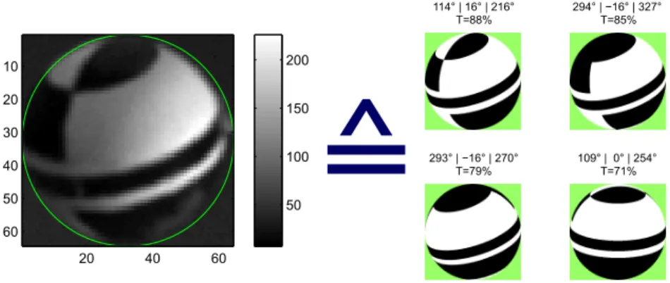
s illustrated in igwe therefore developed a novel measurement technique which can follow the full six degrees of freedom – i.e. position and absolute orientation – of a sphere advected by the ow he angular and linear velocity and acceleration are then the derivatives thereof
he position is carried out with standard particle tracking techniques and two highspeed video cameras racking the absolute orientation of the particle is much more challenging both because of the speci cs of angular variables and because of the speci c algorithmic requirements n contrast to the previous techniques we simply paint the particle with a suitable layout and then retrieve its orientation by a pattern recognition algorithm or algorithmic efficiency and robustness this is not done step by step but for the entire trajectory using a global optimization scheme
his chapter is organized as follows
> e present the experimental setup section
> ext the tracking of several particles is explained section
> he orientation tracking is presented in three steps after establishing important features of the orientation algebra in section the actual algorithm is explained section and tested section
> summary of the data runs is given at the end of this chapter
ome parts follow tightly our article published in eview of cienti c nstruments owever some parts contain more technical details now and information on the tracking of several particles is added or readability some calculations are moved to the annexes
particle propellers cooling circuit b) c) a) d) camera von-Karman mixer camera LED spots
Figure 3.2:ketch of the experimental setupa)sketch of the camera arrangementb) rst version of the von ármán mixerc)upgraded stainless steel version the cooling circuit is now integrated into the metal walls d)a textured particle at different orientations
3.1 Experimental Setup
3.1.1 Von Kármán flow
turbulent ow is generated in the gap between two either co or counterrotating im pellers of radius R = 9.5 cm ∼= 10cm tted with straight blades 1 cm in height he ow domain in between the impeller has characteristic length H = 2R = 20 cm n order to be able to perform direct optical measurements the container is build with at lexiglas olymethyl methacrylate side walls so that the cross section of the vessel is square he total volume is 11.4 l small opening at the top enables us to conveniently add or remove particles from the container ore details on von ármán swirling ow can be found in section and a sketch of the setup is provided in ig ince parts of the apparatus served already in the thesis of icolas ordant and his successor oann asteuil it is still calledKLACshort for von Kármán Lagrangian Acoustics
he working uid – either deionized water or a nely tuned waterglycerol mixture – is chosen such that its density matches the density of the particle cryothermostat con tinuously pumps water of wellcontrolled temperature through a cooling circuit thereby controlling the uids temperature fast degassing can be achieved by heating the uid to 65◦ while the motors and the lter system are running ur lter system consists
simply of a centrifugal pump which pumps uid from a bubble trap through a lter back into the apparatus two high points of the vessel are connected back to the bubble trap he plumbing consist mainly of standard garden hose from the store and ardena quick connectors valves etc all made of plastic
t should be noted that the apparatus was upgraded the rst version was built mainly with brass parts and the propellers were driven by motors mounted to a 1 : 2.5 reductor owever this setup is limited to noncorrosive uids herefore all parts are now made of stainless steel he propellers are now directly driven by brushless motors eroyomer each controlled by a variator e house both in a control cabinet he improved apparatus is easier to use and able to work with corrosive working uids e.g. a potassium salt water mixture which is less viscous than the waterglycerol mixture second apparatus is brie y used in this thesis the Lagrangian Exploration Module LEM here twelve independently driven impellers produce turbulence in a closed icosahedral water tank of 140 l and it was shown that this apparatus creates homogeneous isotropic turbulence with little mean ow urther details are found in sectionand in e estimate the energy injection rate ε by measuring the active power of the delivered motors in water and in air the active power is a direct output of the variators ig
shows the energy injection rate for co and counterrotating impellers or comparison we further provide ε in the ere ε was obtained from measurements
in the center of the apparatus and independently from the active power injected by the twelve motors he two energy injection rates differ by a factor of 20 imilar discrepancy between the two methods of determining ε has been noted in the apparatus in öttin gen too
100 101 10−2
10−1 100 101
Propeller frequency fprop [Hz]
energy injection rate [m
2 .s −3 ] contra−rot co−rot LEM (center) LEM (motors) f3
Figure 3.3:nergy injection rate ε for the ε is based on the energy consumption of the motors n the agrangian xploration odule ε was obtained from
measurements in the center of the apparatus and independently from the total energy injected by the motors imilar discrepancy between the two methods of determining εhas been noted in the apparatus in öttingen too
3.1.2 Particles
wo types of particles have been used
PolyAmid spheres olid white olymid spheres with the following diameters D = 6mm, 10 mm, 15 mm, 18 mm, and 24 mm accuracy 0.01 mm arteau emarié rance were used heir density is ρp = 1.14 g. cm−3 and can be
matched by addition of glycerol to water
Instrumented particles he instrumented particle which is explained in detail in chap ter consists of a 1capsule embarking a circuit which continuously transmits the signal of a accelerometer to an exterior receiver he capsules color is light gray its total density is close to that of water and can be adjusted by adding weight inside
n both cases the density mismatch measured from sedimentation speeds is found to be of the order of ∆ρ /ρ = 10−4 n order to track the orientation the particle is textured black and white by hand using blackink permanent marker exture as well as suitable
pens and nail polish2 have been identi ed by trial and error methods est results were obtained with dding industry permanent marker but in general inks which are not watersoluble perform well igd)shows a textured sphere at four different views he particles are left unpainted white if we just aimed on measuring the translation
3.1.3 Image acquisition & processing
he motion is tracked by two highspeed video cameras hantom ision esearch which record synchronously two views at approximately degree he ow is illumi nated by high power s and sequences of –bit gray scale images are recorded at a sufficiently high frame rate see table page t should be stressed that a short exposure time is crucial for observing a sharp round shape in the movies oth cameras and illumination are mounted to a custommade structure made of aluminum pro les oschexroth and ewport
oth cameras observe the measurement region with a resolution of approximately 650× 650 pixels covering a volume of 15× 15 × 15 [cm] corresponding to 4.2 pixel/mm
ence the particle diameter ranges 25 to 110 pixels
n our con guration the camera can store on the order of 15 000 frames in onboard memory thus limiting the duration of continuous tracks he movies are downloaded to a waiting to be processed he processing is done on a gaming with a state of the art graphics card he code is written in atlab using the image and signal pro cessing toolboxes as well as the sychtoolbox extension which provide pen wrappers for atlab ur image processing is mostly based on the documentation of the atlabs image processing toolbox the book Morphological image analysis: principles and applications nspiration was further found on eter ovesis web site and atlab entral
2ail polish was abandoned because it alters the surface roughness of the particle
3.2 Position Tracking
lthough the identi cation of a large sphere from the camera images causes no particular conceptual difficulty the fact that the sphere is textured raises some practical issues simple thresholding returns only either the white or the black part of the particle e ections from the impellers continuously change the background and small impurities in the ow and possible bubbles add sharp gradient noise to the images urthermore the illumination of the ow is not perfectly uniform and thus shadows as well as re ections occur s the experiment evolved over the time of this thesis light conditions working uid and unfortunately also the scratches on the box changed ence the arrangement of light camera and background as well as the image processing were carefully adjusted for each experiment n either case we compute the background view as the average of an equally distributed subset of its images for each movie of each camera
hree different con gurations were explored within the scope of this thesis3
> several unpainted white particles with different diameters in front of a dark back ground
> one painted particle in front of a light background
> several painted particles in front of a light background all particles having a clearly different diameter associated to a speci c unique texture
Unpainted Particles oth cameras are equipped with a 90 mm macro objective am ron and placed at 1.5 m distance from the center of the vessel ence the diameter of a particles projection varies by less than 10 inside the apparatus e therefore estimate the area Apart covered by particles beforehand or each frame we then subtract the back
ground and threshold such that at least Apart pixels are white or round unconnected
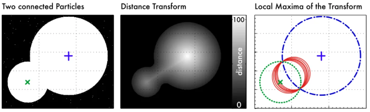
blobs we directly save their location (x, y) on the image in pixels plus their diameter 2 r the deviation from the spherical shape serves as an error estimator onnected blobs are split using the maxima of the distance transform of the blob sketch of the blobsplitting is provided in ig
One textured particle or one painted particle we rst subtract the background and perform a Difference of Gaussians blob detection he threshold is adjusted by hand for each camera and light arrangement e then identify blobs with a round shape and a diameter close to that of the particle hadows bubbles and re ections might be found during blob detection because of their sharp separation from the background but they are of uniform texture and hence characterized by a small value of the variance of light intensity across the blob he blob with highest variance and closest resemblance to a sphere is considered to be the particle he precise position of the particle is re ned using a Canny edge detection or standard deviation lter in a tight region around the blob gain
3he temporal order is slightly different we rst worked on one painted then several unpainted and
Two connected Particles Distance Transform Local Maxima of the Transform
0
distance
100
Figure 3.4:ketch of the lobsplitting technique verlapping particles form a blob he distance transform then returns for each white pixel the euclidian distance to the closest black pixel leaning can be achieved by rejecting all pixels with a distance smaller than the smallest expected particle radius he local maxima of the distance transform are possible particle positions with their associated radii often more maxima than particles are detected and one has to remove artifacts tarting from the largest radius one itera tively excludes wrong detections which are within a bigger particle solidredcircles ne obtains position (x, y) and radius r of the remaining real particles dottedanddashed
circle
for each time step we record the position (x, y) of the particle on the image in pixels plus its diameter 2 r the deviation from the spherical shape serves as an error estimator t is further necessary to store a precise crop of the particle image in order to extract its orientation
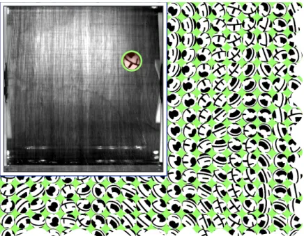
Several textured particles he technique for several painted particles combines ideas from the former two cases iven that the texture strongly deviates from the background a sliding standard deviation lter returns regions of high contrast corresponding to the edges of the particle and its texture hysteresis thresholding based on an estimate of the area covered with particles yields the outlines of the spheres atlab then detects and lls closed outlines f necessary the resulting blob is split osition diameter images and error estimates are stored rom igit becomes clear that if particles overlap the uncertainty in the orientation measurement increases signi cantly e therefore skip these cases and use only the image of the second camera which is typically exploitable
Figure 3.5:verlapping particles the position is extractable but the uncertainty in orien tation increases signi cantly f particles overlap we restrict the orientation measurement to the view of the other camera
Stereo-matching o obtain the particle position in a standard stereomatching technique as sketched in igis employed e model the cameras as pinhole cameras with an additional radial distortion as proposed by sai he projection of a particle on the sensor of the cameras is projected back into where it forms a lineofsight he particles position in is the point which has minimal distance to both linesofsight or setups with two cameras this point can be computed analytically he calibration of the camera contains the position of the camera plus its rotation with respect to the lab coordinate system which is needed later for the orientation processing
Top Camera
Front Camera
Figure 3.6:tereomatching he particle position is the point which has minimal dis tance to both linesofsight
Track assembly he track assembly is straight forward if exactly one particle is placed into the ow he algorithm may temporarily loose the particle for short times because of bad light re ection blurs this is compensated by the large oversampling and gaps of less than frames are interpolated to obtain longer tracks utliers are identi ed using
a leastsquare spline and replaced by an interpolation careful setup and cameras with short exposure time reduce signi cantly the probability of losing particles
f multiple particles are in the ow we still know the possible physical dimensions ex actly he cameras are placed such that the particles projected diameters cover well dis tinct ranges his enables us to convert their observed diameter 2r in pixels to their real particle diameter Dpartin meter articles of the same diameter are then stereomatched
he tracking building is then done in two steps irst particles of the identical size are connected using a earesteighbor track connection which allows short interpolations he tracks break easily when trajectories cross in any of the two cameras due to the large size of the particles or that reason the reconnection algorithm suggested by aitao u is applied t considers both position and velocity at beginning and end of the tracks thereby ensuring a little number misconnections n our case the acceleration of the particle is neglected that corresponds to wa= 0in e further modi ed the search
area from a cylinder to a cone the maximum distance between two tracks separated by ∆t is dmax(∆t) = d0+∆t∆tmax dmax(∆t) = const. was the choice in his modi cation
was added by aitao u cf page in to take into account that the uncertainty of the extrapolation increases with time n a last step we identify and eliminate outliers with a leastsquare spline
s a result we obtain less but signi cantly longer tracks n most cases a particle track now ends when the particle leaves the observation volume
3.3 Orientation Tracking
3.3.1 Math
he parametrization of an angular position in space causes a number of difficulties which are brie y addressed in this section see e.g. for a more complete presentation ne of them is caused by the degeneracy of the axes of rotation for certain orientations the gimbal lock problem nother is the choice of a suitable measure of distance between two orientations n further issue is that mathematically two angular velocities exist hereas ωPdescribes the rotation of the particle with respect to the xed lab coordinate system ωL xes the particle and rotates the lab system his is somewhat similar to quantum mechanics where one has the choice between the eisenberg and the chrödinger picture to incorporate a dependency on time e found no particular use for
ωL in our analysis and name it here just for completeness n the later chapters which analyze and present the results we focus only on the angular velocity which rotates the particle ωP herefore unless otherwise stated the superscriptPis omitted and we always rotate the particle
t should be noted that throughout this manuscript the units of angle degree [◦] radiant [rad] and revolution are equally employed t is left to the reader to convert the units if needed e try to specify the propeller frequency in revolution/s = z and measured angles in degree
3.3.1.1 Describing Orientations
s stated by the uler rotation theorem parameters are needed to describe any rotation in e use here uler angles with the aitryan convention as shown in ig n the transformation from ab to article coordinate system we rst apply a rotation around the z−axis of angle θz followed by a rotation around the intermediate y−axis of
angle θy and last a rotation of angle θx around the new x−axis he rotations work on
the object using a right handed coordinate system and right handed direction of rotation e will denote an orientation triplet by an underscore e.g. θ in order to distinguish them from vectors which are typeset in bold font e.g. ω
he orientation of the object is fully described by an orthogonal 3× 3 matrix R ob tained from the composition of the elementary rotations4
R(θx, θy, θz) = Rx(θx)Ry(θy)Rz(θz) = sθxsθycθcθyzcθ+ cθz xsθz −sθxsθ−cθysθyzsθ+ cθz xcθz −sθsθxycθy −cθxsθycθz+ sθxsθz cθxsθysθz+ sθxcθz cθxcθy
with c = cos ( ) and s = sin ( ) onsequently from any rotation matrix the uler
4n classical mechanics it is common to turn the coordinate system instead of the object which changes