HAL Id: tel-00808623
https://tel.archives-ouvertes.fr/tel-00808623
Submitted on 5 Apr 2013
HAL is a multi-disciplinary open access
archive for the deposit and dissemination of sci-entific research documents, whether they are pub-lished or not. The documents may come from teaching and research institutions in France or abroad, or from public or private research centers.
L’archive ouverte pluridisciplinaire HAL, est destinée au dépôt et à la diffusion de documents scientifiques de niveau recherche, publiés ou non, émanant des établissements d’enseignement et de recherche français ou étrangers, des laboratoires publics ou privés.
To cite this version:
Li Zhou. Statistical problems for SDEs and for backward SDEs. General Mathematics [math.GM]. Université du Maine, 2013. English. �NNT : 2013LEMA1004�. �tel-00808623�
Spécialité : Mathématiques
Option : Statistique
Sujet de la thèse
Problèmes Statistiques pour les EDS
et les EDS Rétrogrades
Présentée par
Li Zhou
Pour obtenir le grade de l’Université du Maine
Soutenue le 28 mars 2013 Composition du Jury :
Dehay Dominique (Université Rennes 2) Rapporteur Hamadene Said (Université du Maine) Examinateur Ji Shaolin (Shandong University) Rapporteur Kabanov Youri (Université de Franche-Comté) Examinateur Kleptsyna Marina (Université du Maine) Examinateur Kutoyants Yury (Université du Maine) Directeur de thèse Nikulin Mikhail (Université Victor Segalen Bordeaux 2) Examinateur
toyants, sans qui cette thèse n’aurait jamais pu voir le jour.
Je suis infiniment reconnaissante envers Youri Koutoyants pour la qualité excep-tionnelle de son encadrement. Sa grande disponibilité, ses conseils avisés et son soutien de chaque instant m’ont été très précieux. Je n’oublierai pas la gentillesse avec laquelle il m’a accueillie dès le début de ma thèse ainsi que toute l’attention qu’il m’a accor-dée. Il m’a en effet guidé, se rendant toujours disponible et partageant avec moi ses expériences et connaissances précieuses, toujours avec une immense générosité. Je lui exprime toute mon admiration, tant sur le plan humain que sur le plan professionnel. Je voudrais témoigner toute ma gratitude à Dominique Dehay et Shaolin Ji qui ont accepté d’être les rapporteurs de cette thèse. Leur lecture attentive et leurs remarques précieuses m’ont permis d’améliorer ce travail. Je remercie très vivement Youri Ka-banov, Mikhail Nikulin, Marina Kleptsyna et Saïd Hamadène qui ont accepté de faire partie du jury lors de la soutenance de ma thèse.
Je voudrais remercier tout les membres de l’équipe «Probabilité et Statistique» de l’université du Maine. Je garderai un excellent souvenir de la bonne ambiance qui règne au sein du laboratoire. Un grand merci à tous mes amis doctorants pour les bons moments que nous avons partagés. Ces années de thèse n’auraient certainement pas été aussi agréables sans mes amis hors laboratoire. Je les remercie tous pour leur convivialité et leurs aides. Je pense tout spécialement à Jing Zhang pour son amitié, je n’oublierai jamais ces instants formidables que nous avons partagés.
Enfin, je ne peux conclure qu’en ayant une pensée toute particulière à ma famille : mon père, ma mère et ma sœur qui, malgré la distance, ont toujours été présents.
tement (goodness-of-fit) pour les modèles de processus de diffusion ergodique. Nous considérons d’abord le cas où le processus sous l’hypothèse nulle appartient à une fa-mille paramétrique. Nous étudions les tests de type Cramer-von Mises et Kolmogorov-Smirnov. Le paramètre inconnu est estimé par l’estimateur de maximum de vraisem-blance ou l’estimateur de distance minimale. Nous construisons alors les tests basés sur l’estimateur du temps local de la densité invariante, et sur la fonction de répar-tition empirique. Nous montrons alors que les statistiques de ces deux types de test convergent tous vers des limites qui ne dépendent pas du paramètre inconnu. Par conséquent, ces tests sont appelés asymptotically parameter free. Ensuite, nous consi-dérons l’hypothèse simple. Nous étudions donc le test du khi-deux. Nous montrons que la limite de la statistique ne dépend pas de la dérive, ainsi on dit que le test est asymptotically distribution free. Par ailleurs, nous étudions également la puissance du test du khi-deux. En outre, ces tests sont consistants.
Nous traitons ensuite le deuxième problème : l’approximation des équations dif-férentielles stochastiques rétrogrades. Supposons que l’on observe un processus de diffusion satisfaisant à une équation différentielle stochastique, où la dérive dépend du paramètre inconnu. Nous estimons premièrement le paramètre inconnu et après nous construisons un couple de processus tel que la valeur finale de l’un est une fonc-tion de la valeur finale du processus de diffusion donné. Par la suite, nous montrons que, lorsque le coefficient de diffusion est petit, le couple de processus se rapproche de la solution d’une équations différentielles stochastiques rétrograde. A la fin, nous prouvons que cette approximation est asymptotiquement efficace.
the model of ergodic diffusion process. We consider firstly the case where the pro-cess under the null hypothesis belongs to a given parametric family. We study the Cramer-von Mises type and the Kolmogorov-Smirnov type tests in different cases. The unknown parameter is estimated via the maximum likelihood estimator or the minimum distance estimator, then we construct the tests in using the local time es-timator for the invariant density function, or the empirical distribution function. We show that both the Cramer-von Mises type and the Kolmogorov-Smirnov type statis-tics converge to some limits which do not depend on the unknown parameter, thus the tests are asymptotically parameter free. The alternatives as usual are nonparametric and we show the consistency of all these tests. Then we study the chi-square test. The basic hypothesis is now simple The chi-square test is asymptotically distribution free. Moreover, we study also power function of the chi-square test to compare with the others.
The other problem is the approximation of the forward-backward stochastic dif-ferential equations. Suppose that we observe a diffusion process satisfying some sto-chastic differential equation, where the trend coefficient depends on some unknown parameter. We try to construct a couple of processes such that the final value of one is a function of the final value of the given diffusion process. We show that when the diffusion coefficient is small, the couple of processes approximates well the solu-tion of a backward stochastic differential equasolu-tion. Moreover, we present that this approximation is asymptotically efficient.
1 Introduction 1
1.1 Test d’Ajustement . . . 2
1.1.1 Les cas des v.a. i.i.d. et des processus de diffusion . . . 2
1.1.2 Résultats principaux . . . 5
1.2 Approximation des EDS Rétrogrades . . . 8
2 On Goodness-of Fit Tests for Diffusion Process 11 2.1 Introduction . . . 11
2.1.1 Auxiliary results . . . 15
2.1.2 A special case . . . 18
2.1.3 Main results . . . 20
2.2 The Cramer-von Mises Type Tests . . . 23
2.2.1 The C-vM type test via the LTE . . . 24
2.2.2 The C-vM type test via the EDF . . . 34
2.2.3 Consistency . . . 40
2.2.4 C-vM test via the MDE . . . 41
2.2.5 Numerical example . . . 50
2.3 The Kolmogorov-Smirnov Type Tests . . . 51
2.3.1 The K-S test via the LTE . . . 53
2.3.2 The K-S test via the EDF . . . 57
2.3.3 Discussions . . . 60
2.3.4 Numerical example . . . 61 i
2.4 The Chi-Square Tests . . . 62
2.4.1 Problem statement . . . 62
2.4.2 The properties of a chi-square test . . . 64
2.4.3 Pitman alternative . . . 67 2.4.4 Example . . . 69 2.4.5 Discussions . . . 69 3 Approximation of BSDE 71 3.1 Introduction . . . 71 3.1.1 Preliminaries . . . 72 3.1.2 Main results . . . 77
3.2 Linear Forward Equation . . . 78
3.2.1 Maximum Likelihood Estimator. . . 78
3.2.2 Approximation process . . . 82
3.3 Nonlinear Forward Equation . . . 84
3.4 On Asymptotic Efficiency of the Approximation . . . 91
3.5 Example . . . 95
3.6 Appendix . . . 99
Introduction
La problématique générale de cette thèse porte sur l’étude des tests d’ajustement de processus de diffusion ergodique et de l’approximation des équations différentielles stochastiques rétrogrades. Dans le chapitre 2, nous étudions le test d’ajustement (goodness-of-fit) pour les modèles de processus de diffusion ergodique. Nous introdui-sons trois types de test : le test de Cramér-von Mises, le test de Kolmogorov-Smirnov et le test du khi-deux. L’objectif de nos travaux dans ce chapitre est de construire les tests consistants, et qui ne dépend asymptotiquement pas soit du paramètre ou soit de la distribution. Une partie des résultats de ce chapitre est issue d’un tra-vail réalisé en collaboration avec Ilia Negri. Le chapitre 3, quant à lui, est consacré à l’étude de l’approximation des équations différentielles stochastiques rétrogrades. Nous construisons un couple de processus dont la valeur finale est une fonction de la valeur finale d’un processus de diffusion donné, dans lequel la dérive dépend d’un paramètre inconnu. Nous montrons ensuite que, lorsque le coefficient de diffusion est petit, le couple de processus se rapproche de la solution d’une équation différentielle stochastique rétrograde. Les résultats de ce chapitre sont issus d’un travail en colla-boration avec Yury A. Kutoyants. Tous nos résultats sont illustrés numériquement par la méthode numérique.
1.1
Test d’Ajustement
1.1.1
Les cas des v.a. i.i.d. et des processus de diffusion
Nous rappelons dans un premier temps le problème de test d’ajustement pour le cas d’observations Xn = (X
1, . . . , Xn) de variables aléatoires indépendantes et
identiquement distribuées (i.i.d.), dont la fonction de répartition est F (x). On teste l’hypothèse H0 contre l’alternative H1
H0 : F(x) = F∗(x), H1 : F(x)6= F∗(x).
Ce genre de problème a été introduit au début de 20ème
siècle, et a été bien étudié pendant les années 50. Nous citons ici les livres de Cramér [7] et de Lehmann & Romano [32], qui ont introduit différents types de test pour le cas i.i.d.
Cramér [6] et Smirnov [46] ont considéré le test ci-dessous, que l’on appelle main-tenant test de Cramer-von Mises (test de C-vM) :
b ψn,1(Xn) = 1I{ω2 n,1>eε,1}, ω 2 n,1= n Z ∞ −∞ h b Fn(x)− F∗(x) i2 dF∗(x) ,
où bFn(·) est la fonction de répartition empirique, eε,1 est le (1− ε)-quantile de cette
distribution, c’est à dire la solution de l’équation suivante : P©ω2
1 > eε,1
ª
= ε. (1.1) Ils ont donné la limite ω2
1 de la statistique ω2n,1 sous l’hypothèse nulle H0. Ils ont
vérifié que cette limite ne dépend pas de la distribution, le test n’en dépend pas non plus. On dit alors que ce test est asymptotically distribution free (ADF).
Par la suite, dans Kolmogorov [26], le test que l’on appelle maintenant test de Kolmogorov-Smirnov (test de K-S) a été introduit. It a été dévloppé ensuite, par exemple par Smirnov [47], Fasano & Franceschini [16], etc. Ils ont considéré la statis-tique de test ci-dessous
ωn,2 =√nsup x ¯ ¯ ¯ bFn(x)− F∗(x) ¯ ¯ ¯ .
Un résultat similaire à celui de C-vM a été présenté : la statistique ωn,2 converge en
loi vers une variable aléatoire ω2. Alors, le test de K-S a été défini comme :
b
ψn,2(Xn) = 1I{ωn,2>eε,2},
où eε,2 est le (1 − ε)-quantile de la distribution de ω2. Etant donné que ce test ne
dépend pas de la distribution, le test est ADF.
Par la suite, le test du khi-deux a été étudié. Nous citons par exemple, Cramér [7], Cochran [5], Dahiya & Gurland [9], Watson [49] et Greenwood & Nikulin [21]. On partitionne R en r intervalles I1 = (a0, a1], I2 = (a1, a2], ..., Ir = (ar−1, ar), où
−∞ = a0 < a1 < · · · < ar = +∞. On définit pi > 0, la probabilité que X1 prenne
les valeurs dans Ii. Alors, pi = F∗(ai)− F∗(ai−1) > 0 et r P i=1 pi = 1. La statistique est définie comme ωn,3= r X i=0 (vi− npi)2 npi ,
où vi est le nombre des valeurs de l’échantillon qui appartiennent à Ii. Cramer [7] a
montré que, quand n→ ∞, la limite de la distribution de ωn,3 est la loi du khi-deux
avec (r− 1)-degré de liberté, que l’on note χ2(r− 1). Par conséquent, le test
b
ψn,3(Xn) = 1I{ωn,3>eε,3},
où eε,3 est le (1− ε)-quantile de la loi χ2(r− 1), est ADF.
Ensuite, les modèles avec paramètres inconnus ont été considérés. Kac al. [23], Durbin [12], Martynov [37] et [38] ont étudié le test d’hypothèse suivant :
H0 : F(x) = F∗(x, ϑ),
où ϑ est un paramètre inconnu. Darling [10] a défini les tests de C-vM et de K-S sous les formes suivantes :
b ψn,1(Xn) = 1I{ω2 n,1>eε,1}, ω 2 n,1= n Z ∞ −∞ h b Fn(x)− F∗ ³ x, bϑn ´i2 dF∗³x− bϑn ´ , et b ψn,2(Xn) = 1I{ωn,2>eε,2}, ωn,2= √ nsup x ¯ ¯ ¯ bFn(x)− F∗ ³ x, bϑn´¯¯¯ ,
où bϑn est un certain estimateur du paramètre inconnu, les seuils eε,i, pour i = 1, 2,
sont les (1− ε)-quantiles de la distribution limite des statistiques. La limite des sta-tistiques dépend généralement du paramètre inconnu. Mais Darling [10] a vérifié que la limite des deux stastistiques ne depend pas des paramètres inconnus pour certains modèles spécifiés (par exemple les modèles à paramètre d’échelle et à paramètre de position), et certains estimateurs comme l’estimateur de maximum de vraisemblance (EMV). Pour ces cas le test ne dépend pas non plus du paramètre inconnu, et le test est dit asymptotically parameter free (APF).
Le problème similaire existe pour les processus stochastiques en temps continu, largement utilisés en tant que modèle mathématique dans plusieurs domaines. Le test d’ajustement a été étudié par de nombreux auteurs : par exemple, Kutoyants [28] a discuté des possibilités de la construction de ces tests. En particulier, il a considéré la statistique de K-S et celle de C-vM basées sur l’observation continue. Supposons que l’observation XT ={X
t,0≤ t ≤ T } est un processus de diffusion en temps continu
dXt = S (Xt) dt + σ(Xt)dWt, X0, 0≤ t ≤ T, (1.2)
où{Wt, t ≥ 0} est un processus de Wiener, le coefficient de dérive S (·) est inconnu
et le coefficient de diffusion σ(·)2 est connu. Il a considéré les hypothèses suivantes
H0 : S(·) = S∗(·), H1 : S(·) 6= S∗(·).
Il a proposé les tests
ψT(XT) = 1I{ωT>yε}, ωT = sup x √ T ¯ ¯ ¯ bfT(x)− f∗(x) ¯ ¯ ¯ , et ΦT(XT) = 1I{ΩT>Yε}, ΩT = sup x √ T ¯ ¯ ¯ bFT(x)− F∗(x) ¯ ¯ ¯ ,
où bfT(·) est l’estimateur de temps local (ETL) de la densité invariante des
obser-vations, bFT(·) est la fonction de répartition empirique (FRE), f∗(x) et F∗(x) sont
respectivement la fonction de densité invariante et la fonction de répartition inva-riante sous l’hypothèse nulle, yε et Yε sont respectivement le (1− ε)-quantile de la
distribution de limite de ωT et de celle de ΩT. La statistique de K-S pour les
pro-cessus de diffusion ergodiques a été étudiée par Fournie [19] et Fournie & Kutoyants [20]. Toutefois, en raison de la structure de la covariance de la limite de processus, la statistique de K-S définie dans [19] et [20] dépend de la distribution dans les modèles de processus de diffusion. Plus récemment, Kutoyants [29] a proposé une modification de la statistique de C-vM et de K-S pour les modèles de diffusion, qui ne dépendt pas de la distribution. Voir également Dachian & Kutoyants [8] qui ont proposé des tests d’ajustement pour des processus de diffusion et de Poisson non-homogène avec des hypothèses de base simple. Dans le cas des processus d’Ornstein-Uhlenbeck, Ku-toyants [30] a montré que le test de C-vM est APF. Un autre test a été étudié par Negri & Nishiyama [40].
1.1.2
Résultats principaux
Dans le chapitre 2, nous considérons le test d’ajustement pour les processus de diffusion dont l’équation est (1.2). La section 2.1 est consacrée aux conditions et aux résultats auxiliaires relatifs aux processus de diffusion. Dans les sections 2.2 et 2.3, nous étudions le modèle défini par (1.2), plus particulièrement dans le cas où la dérive S(·) dépend d’un paramètre inconnu, et le coefficient de diffusion σ(·)2 = 1.
Nous testons l’hypothèse suivante
H0 : S(x) = S∗(x− ϑ) , ϑ ∈ Θ = (α, β)
où S∗(·) est une fonction connue et le paramètre de shift ϑ est inconnu. Par consé-quent, les coefficients de dérive sous l’hypothèse nulle appartiennent à l’ensemble
S (Θ) = {S∗(x− ϑ) , ϑ ∈ Θ} .
L’alternative est définie comme
où S(Θ) = {S∗(x− ϑ) , ϑ ∈ [α, β]}. La section 2.2 est consacrée au test de type C-vM. Nous estimons le paramètre inconnu via l’EMV ou via l’estimateur de distance minimale (EDM), puis nous construisons deux tests de la manière suivante :
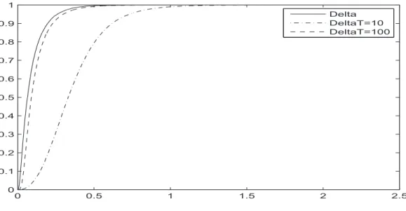
ψT = 1I{δT>dε}, δT = T Z ∞ −∞ ³ b fT(x)− f∗(x− bϑT) ´2 dx, et ΨT = 1I{∆T>Dε}, ∆T = T Z ∞ −∞ ³ b FT(x)− F∗(x− bϑT) ´2 dx,
où bϑT est l’estimateur du paramètre inconnu (l’EMV ou l’EDM). Nous montrons
que sous certaines conditions de régularités, les deux statistiques convergent en loi vers deux variables aléatoires δ et ∆ respectivement. Ainsi dε et Dε sont définies
respectivement comme les (1− ε)-quantiles des distributions de δ et de ∆, c’est à dire les solutions des équations suivantes
P(δ > dε) = ε, P(∆ > Dε) = ε.
Notons que les tests ψT = 1I{δT>dε} et ΨT = 1I{∆T>Dε} sont de taille asymptotique ε,
i.e.
E
∗ψT = ε + o(1), E∗ΨT = ε + o(1),
où E∗ est l’espérance mathématique sous l’hypothèse nulle. En plus nous démontrons dans les théorèmes 2.2.1 et 2.2.2 que les deux tests sont APF. Dans la proposition 2.2.1, nous montrons qu’ils sont consistants.
Dans la section 2.3, nous étudions les tests de type de K-S pour le même modèle. Les tests sont définis comme suit
φT = 1I{λT>cε}, λT = √ T sup x∈R ¯ ¯ ¯ bfT(x)− f∗(x− bϑT) ¯ ¯ ¯ , et ΦT = 1I{ΛT>Cε}, ΛT = √ T sup x∈R ¯ ¯ ¯ bFT(x)− F∗(x− bϑT) ¯ ¯ ¯ .
Nous démontrons dans les théorèmes 2.3.1 et 2.3.2 que les deux tests possèdent les mêmes propriétés que celle de C-vM.
Notons que les tests de C-vM et de K-S dépendent toujours de la dérive. Par consé-quent, nous proposons dans la section 2.4 l’utilisation du test du khi-deux. Supposons que l’observation satisfasse l’équation (1.2), où S(·) est inconnue et σ(·) est connue. Nous testons l’hypothèse nulle suivante
H0 : S(x) = S∗(x) ,
où S∗(·) est une fonction connue. Nous introduisons l’espace L2(f
∗), l’ensemble des
fonctions de carré intégrable avec le poids f∗(·) L2(f ∗) = ½ h(·) : E∗h(ξ0)2 = Z ∞ −∞ h(x)2f∗(x)dx <∞ ¾ .
Soit{φ1, φ2, ...} une base orthonormée complète de cet espace. Nous introduisons alors
l’alternative : pour N ∈ N fixé
H1 : S(·) ∈ SN,
oùSN est le sous-espace des fonctions de carré intégrable suivant
SN = ( S(·) ∈ L2(f∗) ¯ ¯ ¯ ¯ ¯ N X i=1 Z ∞ −∞ φi(x)2fS(x)dx <∞, N X i=1 µZ ∞ −∞ µ S(x)− S∗(x) σ(x) ¶ φi(x)fS(x)dx ¶2 >0 ) . Nous définissons le test du khi-deux comme
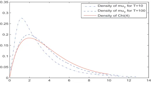
ρT,N = 1I{µT ,N>zε}, où µT,N = N X i=1 µ 1 √ T Z T 0 φi(Xt) σ(Xt) [dXt− S∗(Xt)dt] ¶2 ,
et zε est le (1 − ε)-quantile de loi du khi-deux χ2(N ). Nous démontrons dans le
théorème 2.4.1 que le test du khi-deux est de taille asymptotique ε, qu’il est consistant, et qu’il ne dépend pas de la distribution. De plus, nous étudions le comportement asymptotique du test pour l’alternative de Pitman. Nous donnons dans le théorème 2.4.2 la puissance de ce test. Nous étudions ensuite le cas, plus intétessant, où N → ∞. Nous démontrons dans la proposition 2.4.1 que la limite de la statistique suit une loi normale standard.
1.2
Approximation des EDS Rétrogrades
Par rapport au chapitre 3, nous étudions le problème statistique des équations différentielles stochastiques rétrogrades (EDSR). Supposons que l’on observe un pro-cessus de diffusion XT = {X
t,0 ≤ t ≤ T } satisfaisant une équation différentielle
stochastique (EDS)
dXt= b(Xt)dt + σ(Xt)dWt, 0≤ t ≤ T, X0 = x0.
Pour deux fonctions f (t, x, y, z) et Φ (x) données, la question se pose de construire un couple de processus (Yt, Zt) qui est la solution de l’équation suivante
dYt=−f(t, Xt, Yt, Zt) dt + Zt dWt, 0≤ t ≤ T, (1.3)
avec YT = Φ (XT) comme valeur finale. La solution de ce problème est très connue,
nous citons ici l’article d’El Karoui al. [15]. Dans leur travail, ils ont montré que la solution de cette EDSR est liée à la solution d’une équation différentielle partielle (EDP). En fait, notons u (t, x) la solution de l’équation suivante
( ∂u ∂t + b (x) ∂u ∂x+ 1 2σ(x) 2 ∂2u ∂x2 =−f ¡ t, x, u, σ(x)∂u ∂x ¢ , u(T, x) = Φ (x) . (1.4) En appliquant la formule d’Itô à Yt= u (t, Xt), on obtient
dYt = · ∂u ∂t (t, Xt) + b (Xt) ∂u ∂x(t, Xt) + 1 2σ(X) 2 ∂2u ∂x2 (t, Xt) ¸ dt + ∂u ∂x(t, Xt) σ (Xt) dWt, =−f (t, Xt, Yt, Zt) dt + ZtdWt, Y0 = u (0, x0) ,
où Zt= σ (Xt) u′(t, Xt). Ainsi, le problème (1.3) est résolu et la solution est
Yt = u (t, Xt) , Zt= σ (Xt) u′(t, Xt) .
Le chapitre 3 est consacré au problème suivant
où S et σ sont des fonctions connues et ϑ ∈ Θ ⊂ Rd est un paramètre inconnu.
Dans ce cas, la solution u (t, x, ϑ) de (1.4) dépend également du paramère inconnu. Nous ne pouvons donc plus utiliser Yt = u (t, Xt, ϑ) ni Zt = σ (Xt) u′(t, Xt, ϑ). Par
conséquent, nous considérons le problème de construction d’un couple de processus adaptés ( bYt, bZt), où bYtet bZtsont des approximations de (Yt, Zt). Cette approximation
est réalisée à l’aide de l’EMV bϑ. Nous nous sommes intéressés à une situation où l’erreur de cette approximation est petite. Une des possibilités d’avoir une petite erreur d’approximation est dans un certain sens équivalente à la situation d’avoir une petite erreur d’estimation du paramètre ϑ. Ensuite la continuité de la fonction u(t, x, ϑ) par rapport à ϑ nous donne bYT ∼ YT = Φ (XT).
Nous pouvons avoir la petite erreur d’estimation dans les situations suivantes : soit lorsque T → ∞, soit lorsque σ (·)2 → 0 (à voir par exemple, Kutoyants [28] et [27]). Dans le chapitre 3, nous étudions ce modèle avec un petit bruit, c’est à dire que le coefficient de diffusion tend vers 0. Cela nous permet de garder le temps final T fixé et cette asymptotique est plus facile à traiter.
La section 3.1 est consacrée aux résultats préliminaires. Dans la section 3.2, nous considérons un cas relativement simple, où la dérive S (ϑ, x) est une fonction linéaire de ϑ, le coefficient de diffuson est ε2σ(x)2
et la fonction f (t, x, y, z) est linéaire par rapport à x. Supposons que l’observation XT = {X
t,0 ≤ t ≤ T } satisfait l’EDS
suivante
dXt= ϑh(Xt) dt + εσ(Xt) dWt, X0 = x0, 0≤ t ≤ T. (1.5)
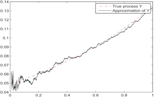
Notre objetif est de construire un couple de processus ( bY , bZ) qui se rapproche de la solution de l’équation
dYt= (k(Xt) + g(Xt) Yt) dt + ZtdWt, 0≤ t ≤ T, YT = Φ(XT). (1.6)
Pour cela, nous estimons tout d’abord ϑ par l’EMV bϑt,εpour tout 0≤ t ≤ T . Ensuite,
les processus approximés sont définis comme : b
où u(t, x, ϑ) est la solution de l’EDP ∂u ∂t + ϑh (x) ∂u ∂x + ε2 2σ(x) 2 ∂2u ∂x2 = k (x) + g (x) u, u(T, x) = Φ (x) . (1.7)
Nous montrons, sous des conditions de régularité, que bYt est proche de Yt pour les
petites valeurs de ε. Dans la section 3.3, nous généralisons le résultat au cas non-linéaire. Dans la section 3.4, nous établissons que l’approximation proposée ci-dessus est asymptotiquement efficace. A la fin, nous illustrons nos résultats par la simulation numérique.
On Goodness-of Fit Tests for
Diffusion Process
2.1
Introduction
We consider the problem of goodness of fit (GoF) test for the model of ergodic diffusion process when this process under the null hypothesis belongs to a given family. In Section 2.2 and 2.3, we study the Cramer-von Mises (C-vM) type and the Kolmogorov-Smirnov (K-S) type statistics for parametrical family. To construct the test, we use the local time estimator (LTE) or the empirical distribution function (EDF). We show that the C-vM type and the K-S type statistics converge in both cases to limits which do not depend on the unknown parameter, so the test is called asymptotically parameter free (APF). In Section 2.4, we study the chi-square test for simple basic hypothesis. We show that the limit of the statistic does not depend on the trend coefficient, that is the test is asymptotically distribution free (ADF). In addition, all of these tests are consistent against any fixed alternatives.
Let us remind the similar statement of the problem in the well known case of the observations of independent identically distributed (i.i.d.) random variables (r.v.) Xn= (X
1, . . . , Xn). Suppose that the distribution of Xj under the basic hypothesis is
F(ϑ, x) = F∗(x− ϑ), where ϑ is some unknown parameter. This kind of parametrical GoF problem has been studied in Kac al. [23], and then developed by many other works. We mention here for example, Darling [10], Martynov [38] and Lehmann &
Romano [32]. In these works, the C-vM type and the K-S type tests are proposed as follows: b ψn,1(Xn) = 1I{ω2 n,1>eε,1}, ω 2 n,1= n Z ∞ −∞ h b Fn(x)− F∗ ³ x− bϑn ´i2 dF∗³x− bϑn ´ , b ψn,2(Xn) = 1I{ωn,2>eε,2}, ωn,2= sup x √ n ¯ ¯ ¯ bFn(x)− F (x − bϑn) ¯ ¯ ¯ ,
where bFn(x) is the EDF and bθn is certain consistent estimator. They proved that
under the basic hypothesis, the statistics ω2
n,1 and ωn,2 converge in distribution to
some random variables ω2
1 and ω2. In addition the limit r.v. ω21 and ω2 do not depend
on ϑ. Thus the threshold eε,i can be calculated as solution of the equation
P©ω2
1 > eε,1
ª
= ε, P{ω2 > eε,2} = ε.
Therefore the tests do not depend on the unknown parameter, that is the C-vM test and the K-S test are all APF. The details concerning this result can be founded in Darling [10] and Kac al. [23]. For more general problems see the works of Durbin [12] or Lehmann & Romano [32].
Otherwise, we are interested in the chi-square test. We mention here the works of Cramer [7], Dahiya & Gurland [9], Watson [49] and Greenwood & Nikulin [21]. For i.i.d. sample{Xn, n ∈ N}, one tests hypothesis H0 that the data form a sample of n
values of a r.v. X with the given probability function f (x). We partition the space of the variable X into r part I1, ..., Ir, and consider the statistic
ωn,3= r X i=0 (vi− npi)2 npi , where pi = P (Ii) > 0 and r P i=1
pi = 1, and vi is the number of sample values which
belong to Ii. Thus Cramer [7] showed that as n −→ ∞, ωn,3 is distributed in a
χ2-distribution with (r− 1)-degrees of freedom (χ2(r− 1)). Thus the test
b
ψn,3(Xn) = 1I{ωn,3>eε,3},
where eε,3 is the (1− ε)-quantile of χ2(r− 1), is ADF, i.e. the test does not depend
A similar problem exists for the continuous time stochastic processes, which are widely used as mathematic models in many fields. The goodness of fit tests (GoF) are studied by many authors. For example Kutoyants [28] discussed some possibilities of construction of such tests. In particular, he considered the K-S statistics and the C-vM Statistics based on the continuous observation. Note that the K-S statistics for ergodic diffusion process were studied in Fournie [19] and in Fournie and Kutoyants [20]. However, due to the structure of the covariance of the limit process, the K-S statistics are not ADF in diffusion process models. More recently Kutoyants [29] has proposed a modification of the K-S statistics for diffusion models that became ADF. See also Dachian and Kutoyants [8] where they propose some GoF tests for diffusion and inhomogeneous Poisson processes with simple basic hypothesis which are all ADF. In the case of Ornstein-Uhlenbeck process Kutoyants showed that the C-vM type tests are APF in [30]. Another test was studied by Negri and Nishiyama [40]. In this work we are interested in the goodness of fit testing problems for composite and simple case. Suppose that the observation XT ={X
t,0≤ t ≤ T } is a
continuous-time diffusion process satisfying
dXt = S (Xt) dt + σ(Xt)dWt, X0, 0≤ t ≤ T, (2.1)
where{Wt, t≥ 0} is a standard Wiener process, the trend coefficient S (·) is unknown
and the diffusion coefficient σ(·)2 is known. We introduce some conditions and
auxil-iary results in this section. Let us remind the following condition, to ensure that the equation (2.1) has a unique weak solution (See Durett [13]).
ES. The function S(·) is locally bounded, the function σ(·)2 is continuous and for
some C > 0,
xS(x) + σ(x)2 ≤ C(1 + x2).
The stochastic process (2.1) has ergodic properties if the functions S(·) and σ(·) satisfy the following two conditions:
RP. V(S, x) = Z x 0 exp ½ −2 Z y 0 S(z) σ(z)2dz ¾ dy→ ±∞, as x → ±∞ and G(S) = Z ∞ −∞ σ(y)−2exp ½ 2 Z y 0 S(z) σ(z)2dz ¾ dy <∞.
That is under these two conditions, the process is recurrent positive and has the following density of invariant law (See Durett [13])
fS(x) = 1 G(S)σ(x)2 exp ½ 2 Z x 0 S(y) σ(y)2dy ¾ .
Denote P as the class of functions having polynomial majorants i.e. P = {h(·) : |h(x)| ≤ C(1 + |x|p)},
with some p > 0. Note that a sufficient condition forRP is A0. The coefficient functions satisfy: σ∓1 ∈ P and
lim
|x|→∞sgn(x)
S(x) σ(x)2 <0.
We introduce also the condition which provides the equivalence of measures defined by different trend coefficient.
EM. The function S(·) and σ(·) satisfy condition ES and the densities fS(·), f0(·)
(with respect to the Lebesgue measure) of the corresponding initial values have the same support.
In this chapter, we study the GoF test for the model (2.1), where some auxiliary results will be required. Therefore, we introduce in the follows some conditions and results about the ergodic diffusion process, including the properties of the maximum likelihood estimator (MLE) and the minimum distance estimator (MDE) for unknown parameter, the LTE for the invariant density function and the EDF.
2.1.1
Auxiliary results
Suppose that we observe an ergodic diffusion process, solution to the following stochas-tic differential equation (SDE)
dXt = S(Xt, ϑ)dt + σ(Xt)dWt, X0, 0≤ t ≤ T, (2.2)
where the functions S(·) and σ(·) are known and the parameter ϑ is unknown. In Kutoyants [28], the author introduced some methods to estimate the unknown pa-rameter. Under the condition A0, the diffusion process is recurrent and its invariant
density fS(x, ϑ) can be written as:
fS(x, ϑ) = 1 G(ϑ)σ(x)2 exp ½ 2 Z x 0 S(y, ϑ) σ(y)2 dy ¾ .
Denote by ξϑ a r.v. having this density fS(x, ϑ), denote by Eϑ the corresponding
mathematic expectation. For any derivable function h(x, ϑ), we denote h′(x, ϑ) the
derivative w.r.t. x and ˙h(x, ϑ) the derivative w.r.t. ϑ.
Let us introduce the MLE bϑT and some properties. We denote L(ϑ, XT) the
log-likelihood ratio L(ϑ, XT) = Z T 0 S(Xt, ϑ) σ(Xt)2 dXt− 1 2 Z T 0 µ S(Xt, ϑ) σ(Xt) ¶2 dt. (2.3) Then the MLE bϑT is defined as the solution of the equation
L(bϑT, XT) = sup θ∈Θ
L(θ, XT).
Let us denote ϑ0 the true value of the unknown parameter, we introduce the
con-ditionA:
A1. The function S(·, ·) is continuously differentiable w.r.t. ϑ, the derivative
˙
S(·, ·) ∈ P and is uniformly continuous in the following sense: lim δ→0|ϑ−ϑsup0|<δ Eϑ 0 ¯ ¯ ¯ ¯ ¯ ˙ S(ξ, ϑ)− ˙S(ξ, ϑ0) σ(ξ) ¯ ¯ ¯ ¯ ¯ 2 = 0.
A2. The Fisher information is positive I(ϑ) = Eϑ Ã ˙ S(ξ, ϑ) σ(ξ) !2 >0, (2.4) and for any ν > 0
inf |ϑ−ϑ0|>δ Eϑ 0 µ S(ξ, ϑ)− S(ξ, ϑ0) σ(ξ) ¶2 >0. We have the following result.
Lemma 2.1.1. (See Kutoyants [28] Theorem 2.8) Let the condition A0 and A be
fulfilled, Then the MLE bϑT is consistent, i.e., for any ν > 0,
lim T →∞ Pϑ 0 © |bϑT − ϑ0| > ν ª = 0, asymptotically normal Lϑ0 ©√ T(bϑT − ϑ0) ª ⇒ N (0, I(ϑ0)−1),
and the moments converge: for p > 0 lim T →∞ Eϑ 0 ¯ ¯ ¯√T(bϑT − ϑ0) ¯ ¯ ¯ p = E|bu|p, where bu is a r.v. of normal distribution N (0, I(ϑ0)−1).
Now we introduce the LTE bfT(x) and the EDF bFT(x). Suppose that the process
observed is a solution to the following SDE
dXt= S(Xt)dt + σ(Xt)dWt, X0, 0≤ t ≤ T, (2.5)
where the trend coefficient S(·) is unknown and the diffusion coefficient σ(·)2 is a
known continuous positive function. Then the invariant density function is fS(x) = 1 G(S)σ(x)2 exp ½ 2 Z x 0 S(y) σ(y)2dy ¾ .
Denote by ξ a r.v. having this density fS(x), denote by ES the corresponding
mathematic expectation. Firstly, we introduce the LTE bfT(x) for this invariant
den-sity function. Let us remind the local time for diffusion process (See Corollary 6.1.9 in Revuz & Yor [45]):
ΛT(x) = lim ε↓0 1 2ε Z T 0 1I{|Xt−x|≤ε}σ(Xt) 2dt.
According to Tanaka’s formula, it can be written as ΛT(x) = 1 T(|XT − x| − |X0− x|) − 1 T Z T 0 sgn(Xt− x)dXt.
Thus we define the LTE for the invariant density function: b
fT(x) =
ΛT(x)
T σ(x)2.
Let us introduce the condition O: O. For some p ≥ 2 ES (¯ ¯ ¯ ¯ FS(ξ)− 1I{ξ>x} σ(ξ)fS(ξ) ¯ ¯ ¯ ¯ p + ¯ ¯ ¯ ¯ Z ξ 0 FS(v)− 1I{v>x} σ(v)2f S(v) dv ¯ ¯ ¯ ¯ p) <∞. Note that under the condition A0, we have the law of large numbers
PS − lim T −→∞ 4fS(x)2 T Z T 0 µF S(Xt)− 1I{Xt>x} σ(Xt)fS(Xt) ¶2 dt = If(S, x) where If(S, x) = 4fS(x)2ES µF S(ξ)− 1I{ξ>x} σ(ξ)fS(ξ) ¶2 . We have the following result
Lemma 2.1.2. (See Kutoyants [28] Theorem 4.11) Let the condition O be fulfilled, then the estimator bfT(x) is consistent and asymptotically normal
LS
n
T1/2( bfT(x)− fS(x))
o
=⇒ N (0, If(S, x)) .
Concerning the EDF
b FT(x) = 1 T Z T 0 1I{Xt<x}dt,
we introduce the condition N :
N . There exists a number p ≥ 2 such that ES (¯¯ ¯ ¯ Z ξ x FS(v∧ x)(FS(v∨ x) − 1) σ(v)2f S(v) dv ¯ ¯ ¯ ¯ p + ¯ ¯ ¯ ¯ FS(ξ∧ x)(FS(ξ∨ x) − 1) σ(ξ)fS(ξ) ¯ ¯ ¯ ¯ p) <∞. Let us denote IF(S, x) = 4ES µ FS(ξ∧ x)(FS(ξ∨ x) − 1) σ(ξ)fS(ξ) ¶2 , then we have the following result
Lemma 2.1.3. (See Kutoyants [28] Theorem 4.6) Let the condition N be fulfilled. Then the EDF bFT(x) is consistent and asymptotically normal.
LS n T1/2( bFT(x)− FS(x)) o =⇒ N (0, IF(S, x)) .
2.1.2
A special case
In Section 2.2 and 2.3, we are interested in the following model. Suppose that the observed ergodic diffusion process satisfies the following SDE
dXt= S(Xt− ϑ)dt + dWt, X0, 0≤ t ≤ T, (2.6)
where ϑ is the unknown shift parameter.
Under the condition A0, the density of the invariant law fS(·, ·) can be calculated
as follows: fS(x, ϑ) = 1 G(ϑ)exp ½ 2 Z x ϑ S(x− ϑ)dy ¾ = exp © 2RϑxS(y− ϑ)dyª R∞ −∞exp © 2RϑyS(z− ϑ)dzªdy = expn2R0x−ϑS(y)dyo R∞ −∞exp © 2R0vS(u)duªdv = f (x− ϑ). (2.7) where f (x) is f(x) = µZ ∞ −∞ exp ½ 2 Z v 0 S(u)du ¾ dv ¶−1 exp ½ 2 Z x 0 S(y)dy ¾ . Let us denote F(x) = Z x −∞ f(y)dy, thus the distribution function of this process is
FS(x, ϑ) = Z x −∞ f(y− ϑ)dy = Z x−ϑ −∞ f(y)dy = F (x− ϑ),
Denote by ξϑ a r.v. with density function f (x− ϑ), denote by Eϑ the corresponding
mathematical expectation. Correspondingly, ξ0 and E0 are respectively the r.v. and
The MLE bϑT is defined as the solution of the equation
L(bϑT, XT) = sup θ∈Θ
L(θ, XT), where L(ϑ, XT) is the log-likelihood ratio
L(ϑ, XT) = Z T 0 S(Xt− ϑ)dXt− 1 2 Z T 0 S(Xt− ϑ)2dt. (2.8) Note that Eϑh(ξϑ− ϑ) = Z ∞ −∞ f(x− ϑ)h(x − ϑ)dx = Z ∞ −∞ f(x)h(x)dx = E0h(ξ0). (2.9)
Therefore, the Fisher information in this case does not depend on the unknown pa-rameter ϑ0, i.e.
I = Eϑ0S′(ξϑ0− ϑ0)
2 = E
0S′(ξ0)2. (2.10)
The condition A in this model can be written as follows:
A1. The function S(·) is continuously differentiable, the derivative S′(·) ∈ P and
it is uniformly continuous in the following sense: lim
ν→0|τ|<νsup
E0¯¯S′(ξ0)− S′(ξ0+ τ )¯¯2 = 0. A2. The Fisher information
I = E0S′(ξ0)2 >0. (2.11)
In addition, for any ν > 0 inf
|τ|>ν
E0¡S(ξ0)− S(ξ0+ τ )¢2 >0.
As that is shown in Lemma 2.1.1, the MLE bϑT is consistent and asymptotically
normal under conditions A0 and A. Let us denote buT =
√ T(bϑT − ϑ0) and define b u=−1 I Z ∞ −∞
S′(y)pf(y)dW (y),
with W (y) = W1(y) for y ∈ R+ and W (y) = W2(−y) for y ∈ R−, where W1 and W2
are independent Wiener processes. Then the asymptotical normality can be written as
From the condition A0, it follows that there exist some constants A > 0 and γ > 0
such that for all|x| > A,
sgn(x)S(x) <−γ. (2.13) It can be shown that for x > A,
f(x) = 1 G(S)exp ½ 2 µZ A 0 + Z x A ¶ S(y)dy ¾ < Ce−2γx. Similar result can be deduced for x <−A, then we have
f(x) < Ce−2γ|x|, for |x| > A. (2.14) Moreover, the LTE bfT(x) is
b fT(x) = 1 T(|XT − x| − |X0− x|) − 1 T Z T 0 sgn(Xt− x)dXt,
and the EDF is
b FT(x) = 1 T Z T 0 1I{Xt<x}dt.
In fact, these estimators of the invariant density and the invariant distribution function are consistent and asymptotically normal under conditionA0. This will be
proved in section 2.2.
2.1.3
Main results
Suppose that we observe an ergodic diffusion process
dXt= S(Xt)dt + dWt, X0, 0≤ t ≤ T. (2.15)
where the trend coefficient S(·) is unknown. We propose three types of GoF test. In section 2.2, we are interested in the following hypotheses test problem. The basic hypothesis is
H0 : S(x) = S∗(x− ϑ) , ϑ ∈ Θ = (α, β)
where S∗(·) is some known function and the shift parameter ϑ is unknown. Therefore, the trend coefficients under hypothesis belong to the family
S (Θ) = {S∗(x− ϑ) , ϑ ∈ Θ} .
The alternative is defined as
whereS(Θ) = {S∗(x− ϑ) , ϑ ∈ [α, β]}.
Let us fix some ε ∈ (0, 1), and denote by Kε the class of tests ψT of asymptotic size
ε, i.e.
E∗ψT = ε + o(1),
where E∗ is the mathematical expectation under the basic hypothesis.
We introduce two C-vM type tests. In the first test, we use the LTE bfT(x) and the
MLE bϑT. The statistic is defined as the following integral
δT = T Z ∞ −∞ ³ b fT(x)− f∗(x, bϑT) ´2 dx,
where f∗(·, ·) is the invariant density function under hypothesis H0. We show that
under hypothesis H0, it converges in distribution to some r.v. δ which does not
depend on ϑ. Thus we define the C-vM type test as ψT = 1I{δT>dε},
with dε the (1− ε)-quantile of the distribution of δ, i.e. dε is the solution of the
following equation
P(δ > dε) = ε.
We show in Section 2.2 that the test ψT belongs to Kε, is consistent and is APF.
The second C-vM type test is based on the EDF bFT(x) and the MLE bϑT:
ΨT = 1I{∆T>Dε}, ∆T = T Z ∞ −∞ ³ b FT(x)− F∗(x, bϑT) ´2 dx,
where F∗(·, ·) is the invariant distribution function under hypothesis H0. The statistic
∆T converges in distribution to some r.v. ∆ which does not depend on ϑ, and Dε is
the (1− ε)-quantile of the distribution of ∆. We obtain that the test ΨT belongs to
Kε and is APF.
In Section 2.3, we study the same hypotheses testing problem, but for the K-S test. We introduce two tests via the LTE bfT(x) and the EDF bFT(x):
φT = 1I{λT>cε}, ΦT = 1I{ΛT>Cε},
where the statistics
λT = √ Tsup x∈R ¯ ¯ ¯ bfT(x)− f∗(x− bϑT) ¯ ¯ ¯ , ΛT = √ T sup x∈R ¯ ¯ ¯ bFT(x)− F∗(x− bϑT) ¯ ¯ ¯ .
These statistics converge in distribution to certain r.v. λ and Λ respectively, which do not depend on ϑ. Thus cε and Cε are defined respectively as the (1− ε)-quantile
of the distribution of λ and Λ. We show that these tests φT and ΦT belong to Kε,
are consistent and are all APF.
In Section 2.4, we study the chi-square test. Suppose that we observe an ergodic diffusion process
dXt= S(Xt)dt + σ(Xt)dWt, X0, 0≤ t ≤ T. (2.16)
We test the following basic hypothesis:
H0 : S(x) = S∗(x) ,
where S∗(·) is some known function. We denote always the invariant density function under the basic hypothesis as f∗(·). Let us introduce the space L2(f
∗) of square
integrable functions with weights f∗(·): L2(f∗) = ½ h(·) : Eh(ξ0)2 = Z ∞ −∞ h(x)2f∗(x)dx <∞ ¾ .
Denote by{φ1, φ2, ...} a complete orthonormal basis in the space L2(f∗). We test the
hypothesisH0 against the alternative
H1,N : S(·) ∈ SN,
whereSN is the subspace of square integrable functions such that for fixed N ∈ N,
SN = ( S(·) ∈ L2(f∗) ¯ ¯ ¯ ¯ ¯ N X i=1 Z ∞ −∞ φi(x)2fS(x)dx <∞, N X i=1 µZ ∞ −∞ µ S(x)− S∗(x) σ(x) ¶ φi(x)fS(x)dx ¶2 >0 ) . The chi-square test will be denoted as
ρT,N = 1I{µT ,N>zε}, µT,N = N X i=1 ηT,N2 where ηT,N = 1 √ T Z T 0 φi(Xt) σ(Xt) [dXt− S∗(Xt)dt],
and zε the (1− ε)-quantile of χ2(N ).We obtain that the test ρT,N belongs to Kε, is
consistent and that it is ADF.
After that, we study the chi-square test for the statistic that N → ∞. We define the statistic νT,N = 1 √ 2N N X i=1 ¡ ηT,N2 − 1¢,
which will be proved to converge to normal distribution N (0, 1) when T → ∞ and N → ∞. Thus the test ρT,N = 1I{νT ,N>Zε}, with Zε the (1− ε)-quantile of N (0, 1)
belongs toKε, is consistent and ADF.
2.2
The Cramer-von Mises Type Tests
This section is based on the work [41]
Suppose that we observe an ergodic diffusion process, solution to the following stochastic differential equation
dXt= S(Xt)dt + dWt, X0, 0≤ t ≤ T. (2.17)
We want to test the following null hypothesis
H0 : S(x) = S∗(x− ϑ) , ϑ ∈ Θ,
where S∗(·) is some known function and the shift parameter ϑ is unknown. We suppose that 0∈ Θ = (α, β). Let us introduce the family
S (Θ) = {S∗(x− ϑ) , ϑ ∈ Θ = (α, β)} .
The alternative is defined as
H1 : S(·) 6∈ S(Θ),
whereS(Θ) = {S∗(x− ϑ) , ϑ ∈ [α, β]}.
We suppose that the trend coefficients S (·) of the observed diffusion process under both hypotheses satisfy the conditionsEM, ES and A0.
Remind that under these conditions the diffusion process is recurrent and its in-variant density fS∗(x, ϑ) under hypothesisH0 can be given explicitly as (2.7). Let us
denote f∗(x) = 1 G(S∗)exp ½ 2 Z x 0 S∗(y)dy ¾ .
then fS∗(x, ϑ) = f∗(x− ϑ). Denote by ξϑ a r.v. having this density f∗(x− ϑ), denote
by Eϑ the mathematical expectation. Moreover the unknown parameter is estimated
by the MLE bϑT
L(bϑT, XT) = sup θ∈Θ
L(θ, XT),
with L(ϑ, XT) the log-likelihood ratio (2.8). Remind that we have in Lemma 2.1.1,
under the conditionsA0 andA, the MLE bϑT is consistent and asymptotically normal.
2.2.1
The C-vM type test via the LTE
To test the hypothesis H0, we propose in this subsection the C-vM type test basing
on the MLE bϑT and the LTE bfT(x)
b fT(x) = 1 T(|XT − x| − |X0− x|) − 1 T Z T 0 sgn(Xt− x)dXt.
Let us denote the statistic as follows δT = T Z ∞ −∞ ³ b fT(x)− f∗(x− bϑT) ´2 dx.
We show that under hypothesis H0, the statistic δT converges in distribution to
δ = Z ∞ −∞ ÃZ ∞ −∞ Ã 2f∗(x)F∗(y)p− 1I{y>x} f∗(y) − 2 IS∗(x)f∗(x)S ′ ∗(y) p f∗(y) ! dW (y) !2 dx, (2.18) with W (y) = W1(y) for y ∈ R+ and W (y) = W2(−y) for y ∈ R−, where W1 and W2
are independent Wiener processes. The C-vM type test is defined as ψT = 1I{δT>dε},
where dε is the (1− ε)-quantile of the distribution of δ, that is the solution of the
following equation
P³δ≥ dε´= ε. (2.19) The main result for the C-vM test via the LTE bfT(x) is the following:
Theorem 2.2.1. Let the conditions ES, A0 and A be fulfilled, then the test ψT =
Note that neither δ nor dε depends on the unknown parameter, this allows us to
conclude that the test is APF. To prove this result, we have to introduce three lemmas which will be given later. All these lemmas are given under the assumption that the hypothesisH0 is true. Let us define ηT(x) = √ T ³fbT(x)− f∗(x− ϑ0) ´ . According to Kutoyants [28] Theorem 4.11, if the hypothesisH0 is true, we have the following representation
ηT(x) = √ T( bfT(x)− f∗(x− ϑ0)) = −2f∗(x√− ϑ0) T Z XT X0 µ F∗(y− ϑ0)− 1I{y>x} f∗(y− ϑ0) ¶ dy +2f∗(x√− ϑ0) T Z T 0 µF ∗(Xt− ϑ0)− 1I{Xt>x} f∗(Xt− ϑ0) ¶ dWt. (2.20) Let us put
M(y, x) = 2f∗(x)F∗(y)− 1I{y>x} f∗(y) . Then ηT(x) can be written as
ηT(x) = 1 √ T Z T 0 M(Xt− ϑ0, x− ϑ0)dWt − √1 T Z XT X0 M(y− ϑ0, x− ϑ0)dy. (2.21) We state that
Lemma 2.2.1. Let the condition A0 be fulfilled, then
Z ∞ −∞ E0 µZ ξ0 0 M(y, x)dy ¶2 dx <∞. Proof. Applying the estimate (2.14), for x > A,
E0 µZ ξ0 0 M(y, x)dy ¶2 = 4f∗(x)2 Z ∞ −∞ µZ z 0 F∗(y)− 1I{y>x} f∗(y) dy ¶2 f∗(z)dz = 4f∗(x)2 µZ −A −∞ + Z A −A + Z x A ¶ µZ z 0 F∗(y) f∗(y)dy ¶2 f∗(z)dz +4f∗(x)2 Z ∞ x µZ x 0 F∗(y) f∗(y)dy + Z z x F∗(y)− 1 f∗(y) dy ¶2 f∗(z)dz
Further, f∗(x)2 Z −A −∞ µZ z 0 F∗(y) f∗(y)dy ¶2 f∗(z)dz = f∗(x)2 Z −A −∞ µµZ −A z + Z 0 −A ¶ F∗(y) f∗(y)dy ¶2 f∗(z)dz ≤ f∗(x)2 Z −A −∞ µZ −A z Z y −∞ 1 G(S∗)exp µ −2 Z y u S∗(v)dv ¶ dudy + C1 ¶2 f∗(z)dz ≤ f∗(x)2 Z −A −∞ µ C2 Z −A z Z y −∞ e−2γ(y−u)dudy + C1 ¶2 f∗(z)dz ≤ Cf∗(x)2 Z −A −∞ (1 + z)2f∗(z)dz ≤ Cf∗(x)2 ≤ Ce−4γx, moreover f∗(x)2 Z x A µZ z 0 F∗(y) f∗(y)dy ¶2 f∗(z)dz ≤ Z x A µµZ A 0 + Z z A ¶ f∗(x) f∗(y)dy ¶2 f∗(z)dz ≤ Z x A µ C1f(x) + C2 Z z A e−2γ(x−y)dy ¶2 f∗(z)dz ≤ Z x A ¡ C1e−2γx+ C2′e−2γ(x−z)− C2′e−2γ(x−A) ¢2 · Ce−2γzdz ≤ e−4γx Z x A ¡ C3e2γz + C4e−2γz ¢ dz ≤ Ce−2γx, and finally f∗(x)2 Z ∞ x µZ z x F∗(y)− 1 f∗(y) dy ¶2 f∗(z)dz = f∗(x)2 Z ∞ x µZ z x 1− F∗(y) f∗(y) dy ¶2 f∗(z)dz ≤ Cf∗(x)2 Z ∞ x µZ z x Z ∞ y e−2γ(u−y)dudy ¶2 e−2γzdz ≤ Cf∗(x)2 Z ∞ x (z− x)2e−2γzdz≤ Cf∗(x)2 Z ∞ 0 s2e−2γ(s+x)ds≤ Ce−6γx. Then we have E0 µZ ξ0 0 M(y, x)dy ¶2 ≤ Ce−2γ|x| for x > A. (2.22)
Similar estimate can be obtained for x <−A, therefore the result holds for |x| > A. We obtain finally Z ∞ −∞ E0 µZ ξ0 0 M(y, x)dy ¶2 dx = µZ −A −∞ + Z A −A + Z ∞ A ¶ E0 µZ ξ0 0 M(y, x)dy ¶2 dx ≤ C1 Z −A −∞ e2γxdx + C2+ C3 Z ∞ A e−2γxdx <∞. This result yields directly the conditions O of Lemma 2.1.2:
Eϑ 0M(ξϑ0 − ϑ0, x− ϑ0) 2 = E 0M(ξ0, x− ϑ0)2 <∞, and Eϑ 0 µZ ξϑ0 0 M(y− ϑ0, x− ϑ0)dy ¶2 <∞.
Thus we deduce the convergence and the asymptotical normality of ηT(x). In fact
under the conditionA0, the LTE bfT(x) is consistent and asymptotically normal, that
is ηT(x) = √ T ³fbT(x)− f∗(x− ϑ0) ´ =⇒ η(x − ϑ0), where η(x)∼ N (0, d(x)2), and d(x)2 = 4f∗(x)2E0 µF ∗(ξ0)− 1I{ξ0>x} f∗(ξ0) ¶2 . Moreover E0(η(x)η(y)) = 4f∗(x)f∗(y)E0 á F∗(ξ0)− 1I{ξ0>x} ¢ ¡ F∗(ξ0)− 1I{ξ0>y} ¢ f∗(ξ0)2 ! . Let us define η(x) = Z ∞ −∞
M(y, x)pf∗(y)dW (y).
The distribution of η(x) isN (0, E0M(ξ0, x)2), and we have the following convergence
Remind that as that is shown in Section 2.1.2 buT = √ T(bϑT − ϑ0) converges in distribution to b u=−1 I Z ∞ −∞
S∗′(y)pf∗(y)dW (y). We have
Lemma 2.2.2. Let the conditions A0 and A be fulfilled, then (ηT(x1), ..., ηT(xk), buT)
is asymptotically normal:
L (ηT(x1), ..., ηT(xk), buT) =⇒ L (η(x1− ϑ0), ..., η(xk− ϑ0), bu) ,
for any x ={x1, x2, ..., xk} ∈ Rk.
Proof. The second integral in (2.21) converges to zero, so we only need to verify the convergence for the part of Itô’s integral. Let us denote for simplicity
η0T(x) = √1 T
Z T 0
M(Xt− ϑ0, x)dWt.
It is sufficient to verify that for any x ={x1, x2, ..., xk},
¡
η0T(x1), ..., ηT0(xk), buT
¢
=⇒ (η(x1), ..., η(xk), bu) . (2.24)
Remind that buT can be defined as follows,
ZT(buT) = sup u∈ T ZT(u), T ={u : ϑ + u √ T ∈ Θ}, (2.25) where ZT(u) = dPT ϑ+ u √ T dPT ϑ (XT) = exp ½ uΛT − u2 2 I+ rT ¾ . Here ΛT = 1 √ T Z T 0 ˙ S∗(Xt− ϑ0)dWt =− 1 √ T Z T 0 S∗′(Xt− ϑ0)dWt
and rT −→ 0. It was proved in Kutoyants [28], Theorem 2.8 that ZT(·) converges in
distribution to Z(·), where Z(u) = exp ½ uΛ− u 2 2 I ¾ ,
with Λ is a r.v. with normal distribution N (0, I), which can be written as Λ =−
Z ∞ −∞
Therefore
b
uT =⇒ bu =
Λ I.
Take u ={u1, u2, ..., um}. We have to verify that the joint finite-dimensional
distri-bution of YT
YT =
¡
ηT0(x1), ηT0(x2), ..., ηT0(xk), ZT(u1), ZT(u2), ..., ZT(um)
¢ converges to the finite-dimensional distribution of Y
Y = (η(x1), η(x2), ..., η(xk), Z(u1), Z(u2), ..., Z(um)) .
Since that rT −→ 0, we consider only the stochastic term ΛT in ZT(u), so (2.24) is
equivalent to ¡
ηT0(x1), η0T(x2), ..., ηT0(xk), ΛT
¢
=⇒ (η(x1), η(x2), ..., η(xk), Λ) . (2.26)
Take λ ={λ1, λ2, ..., λk+1}, and put
h(y, x, λ) = k X l=1 λlM(y, xl)− λk+1S∗′(y). We have Eϑ 0h(ξϑ0 − ϑ0, x, λ) 2 = E 0h(ξ0, x, λ)2 = E0 à k X l=1 λlM(ξ0, xl)− λk+1S∗′(ξ0) !2 = E0 à k X l=1 2λlf∗(xl) F∗(y)− 1I{ξ0>xl} f∗(ξ0) + λk+1S∗′(ξ0) !2 = k X l=1 k X m=1 4λlλmf∗(xl)f∗(xm)E0 µ (F∗(ξ0)− 1I{ξ0>xl})(F∗(ξ0)− 1I{ξ0>xm}) f2 ∗(ξ0) ¶ − k X l=1 4λlλk+1f∗(xl)E0 á F∗(ξ0)− 1I{ξ0>xl} ¢ f∗(ξ0) S∗′(ξ0) ! +λ2k+1E0¡S′ ∗(ξ0)2 ¢ <∞. The law of large number gives us
1 T
Z T 0
h(Xt− ϑ0, x, λ)2dt−→ E0h(ξ0, x, λ)2.
1 √ T Z T 0 h(Xt− ϑ0, x, λ)dWt =⇒ N ¡ 0, E0h(ξ0, x, λ)2 ¢ . In addition k P l=1
λlη(xl) + λk+1Λ is a zero mean normal r.v. with variance
E0 Ã k X l=1 λlη(xl) + λk+1Λ !2 = k X l=1 k X m=1 λlλmE0(η(xl)η(xm)) + 2 k X l=1 λlλk+1E0(η(xl)Λ) + λ2k+1E0(Λ)2. Furthermore E0(η(xl)η(xm)) = 4f∗(xl)f∗(xl) Z ∞ −∞
(F∗(y)− 1I{y>xl})(F∗(y)− 1I{y>xm})
f∗(y) dy = 4f∗(xl)f∗(xl)E0 µ (F∗(ξ0)− 1I{ξ0>xl})(F∗(ξ0)− 1I{ξ0>xm}) f2 ∗(ξ0) ¶ , and E0(η(xl)Λ) = −2f∗(xl) Z ∞ −∞ (F∗(y)− 1I{y>xl})S ′ ∗(y)dy = −2f∗(xl)E0 µ F∗(ξ0)− 1I{ξ0>xl} f∗(ξ0) S∗′(ξ0) ¶ , E0(Λ)2 = Z ∞ −∞ S∗′(y)2f∗(y)dy = E0 ¡ S∗′(ξ0)2 ¢ . We find that Eϑ 0h(ξϑ0 − ϑ0, x, λ) 2 = E 0h(ξ0, x, λ)2 = E0 Ã k X l=1 λlη(xl) + λk+1Λ !2 . This yields that
k X l=1 λlηT0(xl) + λk+1ΛT =⇒ k X l=1 λlη(xl) + λk+1Λ.
Lemma 2.2.3. Let the conditions A0 and A be fulfilled, then L ½Z ∞ −∞ ¡ ηT0(x) + buTf∗′(x) ¢2 dx ¾ =⇒ L ½Z ∞ −∞(η(x) + b uf∗′(x))2dx ¾
Proof. Denote ζT(x) = ηT0(x) + buTf∗′(x) and ζ(x) = η(x) + buf∗′(x), we prove the
following properties
i) ∀L > 0, for x, y ∈ [−L, L] and |x − y| ≤ 1, there exists a constant C depending on L, such that
Eϑ
0|ζT(x)
2
− ζT(y)2|2 ≤ C|x − y|. (2.27)
ii) ∀ε > 0, ∃L > 0, such that Eϑ
0
Z
{|x|>L}
ζT(x)2dx < ε, ∀T > 0. (2.28)
In fact i) and Lemma 2.2.2 yield the convergence in every bounded set [−L, L]: L© Z L −L ζT(x)2dx ª =⇒ L© Z L −L ζ(x)2dxª.
Thus i) and ii) along with and Lemma 2.2.2 give us the result of the lemma. First we prove i). We have
Eϑ 0 ¡ ζT(x)2 ¢ ≤ 2Eϑ0η 0 T(x)2+ 2f (x)2Eϑ0ub 2 T ≤ C. Eϑ 0 ¯ ¯ζT(x)2− ζT(y)2 ¯ ¯2 = Eϑ0 ¡ |ζT(x) + ζT(y)|2|ζT(x)− ζT(y)|2 ¢ ≤ CEϑ0|ζT(x)− ζT(y)| 2 ≤ C(f′(x)− f′(y))2Eϑ 0|buT| 2+ E ϑ0|(η 0 T(x)− ηT0(y))|2. (2.29)
For the first part, let us recall the following result, given in Kutoyants [28], page 119: for any p > 0, R > 0, chosen N sufficiently large, we have
PT
ϑ0{|buT|
p > R
} ≤ RCN/pN . Let us denote FT(u) the distribution of |buT|, we have
Eϑ 0|buT| p = Z ∞ 0 updFT(u)≤ 1 − Z ∞ 1 upd[1− FT(u)] ≤ 1 − [1 − FT(1)] + p Z ∞ 1 up−1 CN uN/pdu≤ C. (2.30)
Remind that under the condition A1, S∗ and f∗ are sufficiently smooth. Thus for
x, y ∈ [−L, L] we have
|f∗(x)− f∗(y)| = |f∗′(z)(x− y)| ≤ C|x − y|,
and |f′ ∗(x)− f∗′(y)| = |f∗′′(z)(x− y)| = ¯ ¯4f(z)S2 ∗(z) + 2f∗(z)S∗′(z) ¯ ¯ |x − y| ≤ C|x − y|. So we have (f∗′(x)− f∗′(y))2Eϑ 0|buT| 2 ≤ C|x − y|2. For the second part in (2.39), note that
Eϑ 0|(η 0 T(x)− ηT0(y))|2 = C1Eϑ0 µ 1 √ T Z T 0 (M (Xt− ϑ0, x)− M(Xt− ϑ0, y))dWt ¶2 ≤ CT1 Z T 0 Eϑ 0(M (Xt− ϑ0, x)− M(Xt− ϑ0, y)) 2 dt = C1E0(M (ξ0, x)− M(ξ0, y))2. Suppose that x≤ y, E0(M (ξ0, x)− M(ξ0, y))2 = Z x −∞ µ 2F∗(z) f∗(z)(f∗(x)− f∗(y)) ¶2 f∗(z)dz + Z y x µ 2 1 f∗(z)((1− F∗(z))f∗(x) + F∗(z)f∗(y)) ¶2 f∗(z)dz + Z ∞ y µ 21− F∗(z) f∗(z) (f∗(x)− f∗(y)) ¶2 f∗(z)dz ≤ C1(x− y)4+ C2(x− y) + C3(x− y)2 ≤ C(y − x).
Similar result holds for x > y. Then we obtain Eϑ 0 ¯ ¯η0 T(x)2− ηT0(y)2 ¯ ¯2 ≤ C|x − y|, x, y ∈ R. Thus we have Eϑ 0 ¯ ¯ζT(x)2− ζT(y)2 ¯ ¯2 ≤ C|x − y|. Now we prove ii). As in Lemma 2.2.1, we have deduced that
Thus for L > A, Eϑ 0 Z ∞ L ¡ ηT0(x)¢2dx = Eϑ0 Z ∞ L µ 1 √ T Z T 0 M(Xt− ϑ0, x)dWt ¶2 dx ≤ C Z ∞ L E0M(ξ0, x)2dx≤ C Z ∞ L e−2γxdx≤ Ce−2γL. Note that f′
∗(x) = 2S∗(x)f∗(x) and along with (2.30) we have
Z ∞ L Eϑ 0 ¡ η0T(x)− f∗′(x)buT ¢2 dx ≤ Z ∞ L ¡ 2Eϑ0ηT(x) 2+ 2f′ ∗(x)Eϑ0ub 2 T ¢ dx ≤ Z ∞ L Ce−2γxdx = Ce−2γL. For any ε > 0, take L =−ln(ε/C)2γ ∨ A, hence we obtain (2.28). Proof of Theorem 2.2.1. We have δT = T Z ∞ −∞ ( bfT(x)− f∗(x− bϑT))2dx = T Z ∞ −∞ ³ ( bfT(x)− f∗(x− ϑ0)) + (f∗(x− ϑ0)− f∗(x− bϑT)) ´2 dx = Z ∞ −∞ ³√ T( bfT(x)− f∗(x− ϑ0)) + √ T(bϑT − ϑ0)f∗′(x− eϑT) ´2 dx = Z ∞ −∞ ³ ηT(x) + buTf∗′(x− eϑT) ´2 dx,
where eϑT is between ϑ0 and bϑT which comes from the mean value theorem. Note that
Eϑ 0 Z ∞ −∞ ³ b u2T|f′ ∗(x− eϑT)− f∗′(x− ϑ0)|2 ´ dx = Eϑ0 Z ∞ −∞ ³ b u2Tf∗′′(x− ¯ϑT)2(eϑT − ϑ0)2 ´ dx. The smoothness of S∗(·) and so that of f′′(·) give us the convergence
Eϑ 0 Z ∞ −∞ ³ b u2T|f∗′(x− eϑT)− f∗′(x− ϑ0)|2 ´ dx−→ 0.
Applying Lemma 2.2.1 and Lemma 2.2.3 we get δT = Z ∞ −∞ ¡ η0T(x− ϑ0) + buTf∗′(x− ϑ0) ¢2 dx + o(1) =⇒ Z ∞ −∞ (η(x− ϑ0) + buf∗′(x− ϑ0))2dx = Z ∞ −∞(η(y) + b uf∗′(y))2dy = Z ∞ −∞(η(y) + 2b uS∗(y)f∗(y))2dy = δ. Note that the limit of the statistic δ does not depend on ϑ0, and the test ψT = 1I{δT≥dε}
with dε defined by P ³ δ ≥ dε ´ = ε belongs toKε.
2.2.2
The C-vM type test via the EDF
We introduce in this subsection the C-vM type test in using the EDF: b FT(x) = 1 T Z T 0 1I{Xt<x}dt.
Let us define the statistic ∆T = T Z ∞ −∞ ³ b FT(x)− F∗(x− bϑT) ´2 dx, and its limit in distribution
∆ = Z ∞ −∞ ÃZ ∞ −∞ Ã 2F∗(y)F∗(x)p − F∗(y∧ x) f∗(y) − 1 If∗(x)S ′ ∗(y) p f∗(y) ! dW (y) !2 dx. (2.31) This convergence will be proved later. Thus we propose the C-vM type test
ΨT = 1I{∆T>Dε},
where Dε is the solution of the equation
P ³
∆≥ Dε
´
= ε. (2.32) We have the result
Theorem 2.2.2. Under the conditions ES, A0 and A, the test ΨT = 1I{∆T>Dε}
belongs to Kε and is APF.
Denote ηF T(x) = √ T( bFT(x)− F∗(x− ϑ0)) and H(z, x) = 2F∗(z)F (x)− F∗(z∧ x) f∗(z) .
In Kutoyants [28] Theorem 4.6, the following equality is presented: ηFT(x) = √2 T Z XT X0 F∗((z∧ x) − ϑ0)− F∗(z− ϑ0)F∗(x− ϑ0) f∗(z− ϑ0) dz −√2 T Z T 0 F∗((Xt∧ x) − ϑ0)− F∗(Xt− ϑ0)F∗(x− ϑ0) f∗(Xt− ϑ0) dWt = −√1 T µZ XT 0 H(z− ϑ0, x− ϑ0)dz− Z X0 0 H(z− ϑ0, x− ϑ0)dz ¶ +√1 T Z T 0 H(Xt− ϑ0, x− ϑ0)dWt. (2.33)
We present the following lemma
Lemma 2.2.4. Let the condition A0 be fulfilled, then
Z ∞ −∞ E0 µZ ξ0 0 H(y, x)dy ¶2 dx <∞. Proof. In applying (2.13) we have, for x > A,
1− F∗(x) = C Z ∞ x exp µ 2 Z y 0 S∗(r)dr ¶ dy ≤ Ce−2γx, and 1− F∗(x) f∗(x) ≤ C Z ∞ x e−2γ(y−x)dy ≤ C. For x <−A we have F∗(x)≤ Ce−2γ|x| and we can write
F∗(x) f∗(x) = C Z x −∞ exp(2 Z y x S∗(r)dr)dy ≤ C.
So that for x > A, E µZ ξ0 0 H(z, x)dz ¶2 = 4 Z A −∞ f∗(y) µZ y 0 (F∗(x)− 1)Ff∗(z) ∗(z) dz ¶2 dy +4 Z x A f∗(y) µZ y 0 (F∗(x)− 1)F∗(z) f∗(z)dz ¶2 dy +4 Z ∞ x f∗(y) µZ x 0 (F∗(x)− 1)F∗(z) f∗(z)dz + Z y x F∗(x)F∗(z)− 1 f∗(z) dz ¶2 dy. Note that Z A −∞ f∗(y) µZ y 0 (F∗(x)− 1)F∗(z) f∗(z)dz ¶2 dy = Z A −∞ f∗(y) µZ y 0 (1− F∗(x)) F∗(z) f∗(z)dz ¶2 dy ≤ (1 − F∗(x))2 Z A −∞ y2f∗(y)dy ≤ C(1 − F∗(x))2 ≤ Ce−4γx, Further Z x A f∗(y) µZ y 0 (1− F∗(x)) F∗(z) f∗(z)dz ¶2 dy ≤ Z x A f∗(y) µZ y 0 1− F∗(x) f∗(z) dz ¶2 dy ≤ C Z x A f∗(y) µZ y 0 Z ∞ x e−2γ(u−z)dudz ¶2 dy ≤ C Z x A
f∗(y)e−2γx¡1− e2γy¢dy ≤ C(1 + x)e−2γx,
and Z ∞ x f∗(y) µZ x 0 (1− F∗(x))F∗(z) f∗(z)dz ¶2 dy = Z ∞ x f∗(y) µµZ A 0 + Z x A ¶ (1− F∗(x)) F∗(z) f∗(z)dz ¶2 dy ≤ C Z ∞ x f∗(y) µ (1− F∗(x)) + Z x A 1− F∗(x) f∗(z) dz ¶2 dy ≤ C Z ∞ x f∗(y)(1 + e−4γx)dy ≤ Ce−2γx,
and Z ∞ x f∗(y) µZ y x F∗(x)F∗(z)− 1 f∗(z) dz ¶2 dy ≤ C Z ∞ x (y− x)f∗(y)dy ≤ C(1 + x)e−2γx, thus we have E0 µZ ξ0 0 H(z, x)dz ¶2 ≤ Ce−γx, x > A. (2.34) Similarly we get E0 µZ ξ0 0 H(z, x)dz ¶2 ≤ Ce−γ|x|, x <−A. and E0 µZ ξ0 0 H(z, x)dz ¶2 ≤ C, x ∈ [−A, A]. We obtain finally Z ∞ −∞ E0 µZ ξ0 0 H(y, x)dy ¶2 dx <∞. This inequality allows us to deduce the following bounds
Eϑ 0H(ξϑ0− ϑ0, x) 2 = E 0H(ξ0, x)2 <∞, (2.35) and Eϑ 0 µZ ξϑ0−ϑ0 0 H(z, x)dz ¶2 = E0 µZ ξ0 0 H(z, x)dz ¶2 ≤ ∞, |x| > A. (2.36) Hence we get the asymptotic normality of ηF
T(x): ηFT(x) =⇒ ηF(x− ϑ 0)∼ N (0, E0(H(ξ0, x− ϑ0))2), where we define ηF(x) = Z ∞ −∞
H(y, x)pf(y)dW (y).
As in Lemma 2.2.2 and Lemma 2.2.3, if conditions A and A0 hold, we show the
convergence of the vector (ηF
Lemma 2.2.5. Let the conditions A0 and A be fulfilled, then Lϑ0 ¡ ηTF(x1), ..., ηTF(xk), buT ¢ =⇒ Lϑ0 ¡ ηF(x1− ϑ0), ..., ηFT(xk− ϑ0), bu ¢ for any x ={x1, x2, ..., xk} ∈ Rk.
Proof. We omit the proof since that it is similar as Lemma 2.2.2. Let us define e ηTF(x) = √1 T Z T 0 H(Xt− ϑ0, x)dWt we prove that
Lemma 2.2.6. Let the conditions A and A0 be fulfilled, then
Lϑ0 © Z ∞ −∞ ¡ e ηTF(x) + buTf∗(x) ¢2 dxª =⇒ L ½Z ∞ −∞ ¡ ηF(x) + buf∗(x)¢2dx ¾ . Proof. Denote ζF
T(x) = eηFT(x)− buTf∗(x). Similar as Lemma 2.2.3, we need to
verify
i) ∀ L > 0, for x, y ∈ [−L, L] and |x − y| ≤ 1, there exists C depending on L such that
Eϑ
0|ζ
F
T(x)2 − ζTF(y)2|2 ≤ C|x − y|1/2. (2.37)
ii)∀ ε > 0, ∃L > 0, such that Eϑ
0
Z
{|x|>L}
ζTF(x)2dx < ε, ∀T > 0. (2.38) Firstly we prove i). Note that
Eϑ 0 ¯ ¯ζF T(x)2− ζTF(y)2 ¯ ¯2 ≤ C¡(f∗(x)− f∗(y))4Eϑ 0|buT| 4+ E ϑ0|(eη F T(x)− eηTF(y))|4 ¢1/2 . Moreover, Eϑ 0|(eη F T(x)− eηTF(y))|4 ≤ C1T−2Eϑ0 µ 1 √ T Z ξϑ0−ϑ0 0 (H(z, x)− H(z, y))dz ¶4 + C2T−5/4Eϑ0 µ 1 √ T Z T 0 (H(Xt− ϑ0, x)− H(Xt− ϑ0, y))dWt ¶4 ≤ C1T−2E µ 1 √ T Z ξ0 0 (H(z, x)− H(z, y))dz ¶4 + C2T−1/4E(H(ξ0, x)− H(ξ0, y))4.
Suppose that x≤ y, Eϑ 0(H(Xt, x)− H(Xt, y)) 4 = Z x −∞ F∗(z) f∗(z)(F∗(x)− F∗(y))dz + Z ∞ y F∗(z)− 1 f∗(z) (F∗(x)− F∗(y))dz + Z y x 1 f∗(z)(F∗(z)(F∗(x)− F∗(y)) + (F∗(z)− F∗(x))) dz ≤ C1(x− y)4+ C3(x− y)4+ C2(x− y) and Eϑ 0 µZ ξ 0 H(z, x)− H(z, y)dz ¶4 = 2 Z x −∞ f∗(s) µZ s 0 F∗(z) f∗(z)(F∗(x)− F∗(y))dz ¶4 ds +2 Z y x f∗(s) µZ s x F∗(z)− F∗(x) + F∗(z)(F∗(x)− F∗(y)) f∗(z) dz ¶4 ds +8 Z ∞ y f∗(s) µZ y x F∗(z)− F∗(x) + F∗(z)(F∗(x)− F∗(y)) f∗(z) dz ¶4 ds +8 Z ∞ y f∗(s) µZ s y F∗(z)− 1 f∗(z) (F∗(x)− F∗(y))dz ¶4 ds ≤ C1(y− x)4+ C2(y− x) + C3(y− x)4+ C4(y− x)4.
Similar result for x≥ y. We obtain finally Eϑ 0 ¯ ¯eηF T(x)− eηFT(y) ¯ ¯4 ≤ C|x − y|, Therefore, Eϑ 0 ¯ ¯ζF T(x)2− ζTF(y)2 ¯ ¯2 ≤ |x − y|1/2.
Now we prove ii). Thanks to Lemma 2.2.4, we have Eϑ 0 ¯ ¯eηF T(x) ¯ ¯2 ≤ Ce−γ|x|, x > A. (2.39) Hence for L > A, Z ∞ L Eϑ 0 ¡ e ηTF(x)− f∗(x)buT ¢2 dx ≤ Z ∞ L ¡ 2Eϑ0η F T(x)2+ 2f∗(x)2Eϑ0ub 2 T ¢ dx ≤ Z ∞ L Ce−γxdx = Ce−γL.