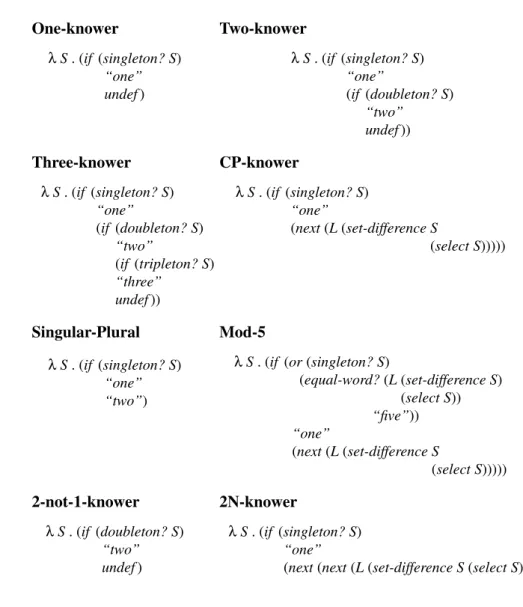
model of conceptual change in number word learning
The MIT Faculty has made this article openly available.
Please share
how this access benefits you. Your story matters.
Citation
Piantadosi, Steven T., Joshua B. Tenenbaum, and Noah D. Goodman.
“Bootstrapping in a Language of Thought: A Formal Model of
Numerical Concept Learning.” Cognition 123, no. 2 (May 2012): 199–
217.
As Published
http://dx.doi.org/10.1016/j.cognition.2011.11.005
Publisher
Elsevier
Version
Author's final manuscript
Citable link
http://hdl.handle.net/1721.1/98844
Terms of Use
Creative Commons Attribution-Noncommercial-NoDerivatives
Detailed Terms
http://creativecommons.org/licenses/by-nc-nd/4.0/
a formal model of conceptual change
in number word learning
Steven T. Piantadosi
Department of Brain and Cognitive Sciences, MIT
Joshua B. Tenenbaum
Department of Brain and Cognitive Sciences, MIT
Noah D. Goodman
Department of Psychology, Stanford University
Abstract
In acquiring number words, children exhibit a qualitative leap in which they transi-tion from understanding a few number words, to possessing a recursive system of interrelated numerical concepts. We present a computational framework for under-standing this inductive leap as the consequence of statistical inference over a suffi-ciently powerful representational system. We provide an implemented model that is powerful enough to learn number word meanings and other related conceptual systems from naturalistic data. The model shows that bootstrapping can be made computationally and philosophically well-founded as a theory of number learning. Our approach demonstrates how learners may combine core cognitive operations to build sophisticated representations during the course of development, and how this process explains observed developmental patterns in number word learning.
Introduction
“We used to think that if we knew one, we knew two, because one and one are two. We are finding that we must learn a great deal more about ‘and’.” [Sir Arthur Eddington]
Cognitive development is most remarkable where children appear to acquire genuinely novel concepts. One particularly interesting example of this is the acquisition of number words. Children initially learn the count list “one”, “two”, “three”, up to “six” or higher, without knowing the exact numerical meaning of these words (Fuson, 1988). They then progress through several
subset-knower levels, successively learning the meaning of “one”, “two”, “three” and sometimes “four”
or two objects when asked, but when asked for three or more will simply give a handful of objects, even though they can recite much more of the count list.
After spending roughly a year learning the meanings of the first three or four words, children make an extraordinary conceptual leap. Rather than successively learning the remaining number words on the count list—up to infinity—children at about age 3;6 suddenly infer all of their mean-ings at once. In doing so, they become cardinal-principal (CP) knowers, and their numerical un-derstanding changes fundamentally (Wynn, 1990, 1992). This development is remarkable because CP-knowers discover the abstract relationship between their counting routine and number word meanings: they know how to count and how their list of counting words relate to numerical mean-ing. This learning pattern cannot be captured by simple statistical or associationist learning models which only track co-occurrences between number words and sets of objects. Under these models, one would expect that number words would continue to be acquired gradually, not suddenly as a coherent conceptual system. Rapid change seems to require a learning mechanism which comes to some knowledge that is more than just associations between words and cardinalities.
We present a formal learning model which shows that statistical inference over a sufficiently powerful representational space can explain why children follow this developmental trajectory. The model uses several pieces of machinery, each of which has been independently proposed to explain cognitive phenomena in other domains. The representational system we use is lambda calculus, a formal language for compositional semantics (e.g. Heim & Kratzer, 1998; Steedman, 2001), com-putation more generally (Church, 1936), and other natural-language learning tasks (Zettlemoyer & Collins, 2007, 2005; Piantadosi, Goodman, B.A., & J.B., 2008). The core inductive part of the model uses Bayesian statistics to formalize what inferences learners should make from data. This involves two key parts: a likelihood function which measures how well hypotheses fit ob-served data, and a prior which measures the complexity of individual hypotheses. We use simple and previously-proposed forms of both. The model uses a likelihood function that uses the size
principle (Tenenbaum, 1999) to penalize hypotheses which make overly-broad predictions. Frank,
Goodman, and Tenenbaum (2007) proposed that this type of likelihood function is important in cross-situational word learning and Piantadosi et al. (2008) showed that it could solve the
sub-set problem in learning compositional semantics. The prior is from the rational rules model of
Goodman, Tenenbaum, Feldman, and Griffiths (2008), which first linked probabilistic inference with formal, compositional, representations. The prior assumes that learners prefer simplicity and re-use in compositional hypotheses and has been shown to be important in accounting for human rule-based concept learning.
Our formal modeling is inspired by the bootstrapping theory of Carey (2009), who proposes that children observe a relationship between numerical quantity and the counting routine in early number words, and use this relationship to inductively define the meanings of later number words. The present work offers several contributions beyond Carey’s formulation. Bootstrapping has been criticized for being too vague (Gallistel, 2007), and we show that it can be made mathematically-precise and implemented by straighforward means1. Second, bootstrapping has been criticized for being incoherent or logically circular, fundamentally unable to solve the critical problem of infer-ring a discrete infinity of novel numerical concepts (Rips, Asmuth, & Bloomfield, 2006, 2008; Rips, Bloomfield, & Asmuth, 2008). We show that this critique is unfounded: given the assumptions of the model, the correct numerical system can be learned while still considering conceptual systems
like those suggested as possible alternatives by Rips, Asmuth and Bloomfield. The model is capable of learning the types of conceptual systems they discuss, as well as others that are likely important for natural language. We also show that the model robustly gives rise to several qualitative phenom-ena in the literature which have been taken to support bootstrapping: the model progresses through three or four distinct subset knower-levels (Wynn, 1990, 1992; Sarnecka & Lee, 2009), does not assign specific numerical meaning to higher number words at each subset-knower level (Condry & Spelke, 2008), and suddenly infers the meaning of the remaining words on the count list after learning “three” or “four” (Wynn, 1990, 1992; Sarnecka & Lee, 2009).
This modeling work demonstrates how children might combine statistical learning and rich representations to create a novel conceptual system. Because we provide a fully-implemented model which takes naturalistic data and induces representations of numerosity, this work requires making a number of assumptions about facts which are under-determined by the experimental data. This means that the model provides at minimum an existence proof for how children might come to numerical representations. However, one advantage of this approach is that it provides a computa-tional platform for testing multiple theories within this same framework—varying the parameters, representational system, and probabilistic model. We argue that all assumptions made are computa-tionally and developmentally plausible, meaning that the particular version of the model presented here provides a justifiable working hypothesis for how numerical acquisition might progress.
The bootstrapping debate
Carey (2009) argues that the development of number meanings can be explained by (Quinian)
bootstrapping. Bootstrapping contrasts with both associationist accounts and theories that posit an
innate successor function that can map a representation of a number N onto a representation of its successor N + 1 (Gallistel & Gelman, 1992; Gelman & Gallistel, 1978; Leslie, Gelman, & Gallistel, 2008). In Carey’s formulation, early number word meanings are represented using mental models of small sets. For instance two-knowers might have a mental model of “one” as {X} and “two” as{X,X}. These representations rely on children’s ability for enriched parallel individuation, a representational capacity that Le Corre and Carey (2007) argue can individuate objects, manipulate sets, and compare sets using 1-1 correspondence. Subset-knowers can, for instance, check if “two” applies to a set S by seeing if S can be put in 1-1 correspondence with their mental model of two,
{X,X}.
In bootstrapping, the transition to CP-knower occurs when children notice the simple rela-tionship between their first few mental models and their memorized count list of number words: by moving one element on the count list, one more element is added to the set represented in the mental model. Children then use this abstract rule to bootstrap the meanings of other number words on their count list, recursively defining each number in terms of its predecessor. Importantly, when children have learned the first few number word meanings they are able to recite many more elements of the count list. Carey argues that this linguistic system provides a placeholder structure which provides the framework for the critical inductive inference. Subset knowers have only stored a few set-based representations; CP-knowers have discovered the generative rule that relates mental representations to position in the counting sequence.
Bootstrapping explains why children’s understanding of number seems to change so drasti-cally in the CP-transition and what exactly children acquire that’s “new”: they discover the simple recursive relationship between their memorized list of words and the infinite system of numerical concepts. However, the theory has been criticized for its lack of formalization (Gallistel, 2007) and
the fact that it does not explain how the abstraction involved in number word meanings is learned (Gelman & Butterworth, 2005). Perhaps the most philosophically interesting critique is put forth by Rips et al. (2006), who argue that the bootstrapping hypothesis actually presupposes the equivalent of a successor function, and therefore cannot explain where the numerical system comes from (see also Margolis & Laurence, 2008; Rips, Asmuth, & Bloomfield, 2008; Rips, Bloomfield, & Asmuth, 2008). Rips, Asmuth, & Bloomfield argue that in transitioning to CP-knowers, children critically infer,
If k is a number word that refers to the property of collections containing n objects, then the next number word in the counting sequence, next(k), refers to the property of collections containing one more than n objects.
Rips, Asmuth & Bloomfield note that to even consider this as a possible inference, children must know how to construct a representation of the property of collections containing n + 1 ob-jects, for any n. They imagine that totally naive learners might entertain, say, a Mod-10 system in which numerosities start over at ten, with “eleven” meaning one and “twelve” meaning two. This system would be consistent with the earliest-learned number meanings and thus bootstrapping number meanings to a Mod-10 system would seem to be a logically consistent inference. Since children avoid making this and infinitely many other possible inferences, they must already bring to the learning problem a conceptual system isomorphic to natural numbers.
The formal model we present shows how children could arrive at the correct inference and learn a recursively bootstrapped system of numerical meanings. Importantly, the model can enter-tain other types of numerical systems like such Mod-N systems, and, as we demonstrate, will learn them when they are supported by the data. These systems are not ruled out by any hard constraints and therefore the model demonstrates one way bootstrapping need not assume specific knowledge of natural numbers.
Rebooting the bootstrap: a computational model
The computational model we present focuses on only one slice of what is undoubtedly a complex learning problem. Number learning is likely influenced by social, pragmatic, syntactic, and pedagogical cues. However, we simplify the problem by assuming that the learner hears words in contexts containing sets of objects and attempts to learn structured representations of mean-ing. The most basic assumption of this work is that meanings are formalized using a “language of thought (LOT)” (Fodor, 1975), which, roughly, defines a set of primitive cognitive operations and composition laws. These meanings can be interpreted analogously to short computer programs which “compute” numerical quantities. The task of the learner is to determine which compositions of primitives are likely to be correct, given the observed data. Our proposed language of thought is a serious proposal in the sense that it contains primitives which are likely available to children by the age they start learning number, if not earlier. However, like all cognitive theories, the particular language we use is a simplification of the computational abilities of even infant cognition.
We begin by discussing the representational system and then describe basic assumptions of the modeling framework. We then present the primitives in the representational system and the probabilistic model.
A formalism for the LOT: lambda calculus
We formalize representations of numerical meaning using lambda calculus, a formalism which allows complex functions to be defined as compositions of simpler primitive functions. Lambda calculus is computationally and mathematically convenient to work with, yet is rich enough to express a wide range of conceptual systems2. Lambda calculus is also a standard formalism in se-mantics (Heim & Kratzer, 1998; Steedman, 2001), meaning that, unlike models that lack structured representations, our representational system can interface easily with existing theories of linguistic compositionality. Additionally, lambda calculus representations have been used in previous com-putational models of learning words with abstract or functional properties (Zettlemoyer & Collins, 2005, 2007; Piantadosi et al., 2008).
The main work done by lambda calculus is in specifying how to compose primitive functions. An example lambda expression is
λ x . (not (singleton? x)). (1)
Each lambda calculus expression represents a function and has two parts. To the left of a period, there is a “λx”. This denotes that the argument to the function is the variable named x. On the right hand side of the period, the lambda expression specifies how the expression evaluates its arguments. Expression (1) returns the value of not applied to (singleton? x). In turn, (singleton? x) is the function singleton? applied to the argument x3. Since this lambda expression represents a function, it can be applied to arguments—in this case, sets—to yield return values. For instance, (1) applied to
{Bob,Joan} would yieldTRUE, but{Carolyn} yieldsFALSEsince only the former is not a singleton set.
Basic assumptions
We next must decide on the appropriate interface conditions for a system of numerical meaning—what types of questions can be asked of it and what types of answers can it provide. There are several possible ways of setting up a numerical representation: (i) The system of numer-ical meaning might map each number word to a predicate on sets. One would ask such a system for the meaning of “three”, and be given a function which is true of sets containing exactly three elements. Such a system would fundamentally represent a function which could answer “Are there
n?” for each possible n. (ii) The system of numerical meaning might work in the opposite direction,
mapping any given set to a corresponding number word. In this setup, the numerical system would take a set, perhaps{duckA, duckB, duckC}, and return a number word corresponding to the size of
the set—in this case, “three”. Such a system can be thought of as answering the question “How many are there?” (iii) It is also possible that the underlying representation for numerical meaning is one which relies on constructing a set. For instance, the “meaning” of “three” might be a function which takes three elements from the local context and binds them together into a new set. Such a function could be cached out in terms of motor primitives rather than conceptual primitives, and could be viewed as responding to the command “Give me n.”
2In fact, untyped lambda calculus could represent any computable function from sets to number words. While we use
a typed version of lambda calculus, our numerical meanings still have the potential to “loop infinitely,” requiring us to cut off their evaluation after a fixed amount of time.
3As in the programming language scheme, function names often include “?” when they return a truth value. In
It is known that children are capable of all of these numerical tasks (Wynn, 1992). This is not surprising because each type of numerical system can potentially be used to answer other questions. For instance, to answer “How many are there?” with a type-(i) system, one could test whether are are n in the set, for n = 1, 2, 3, . . .. Similarly, to answer “Are there n” with a type-(ii) system, one could compute which number word represents the size of the set, and compare it to n.
Unfortunately, the available empirical data does not provide clear evidence for any of these types of numerical representations over the others. We will assume a type-(ii) system because we think that this is the most natural formulation, given children’s counting behavior. Counting appears to be a procedure which takes a set and returns the number word corresponding to its cardinality, not a procedure which takes a number and returns a truth value4.
Importantly, assuming a type-(ii) system (or any other type) only determines the form of the inputs and outputs5—the inputs are sets and the outputs are number words. Assuming a type-(ii) system does not mean that we have assumed the correct input and output pairings. Other conceptual systems can map sets to words, but do it in the “wrong” way: a Mod-10 system would take a set containing n elements and return the n mod 10’th number word.
Primitive operations in the LOT
In order to define a space of possible lambda expressions, we must specify a set of primitive functional elements which can be composed together to create lambda expressions. These primi-tives are the basic cognitive components that learners must figure out how to compose in order to arrive at the correct system of numerical meanings. The specific primitives we choose represent only one particular set of choices, but this modeling framework allows others to be explored to see how well they explain learning patterns. The primitives we include can be viewed as partial imple-mentation of the core knowledge hypothesis (Spelke, 2003)—they from a core set of computations that learners bring to later development. Unlike core knowledge, however, the primitives we assume are not necessarily innate—they must only be available to children by the time they start learning number. These primitives—especially the set-based and logical operations—are likely useful much more broadly in cognition and indeed have been argued to be necessary in other domains. Similar language-like representations using overlapping sets of logical primitives have previously proposed in learning kinship relations and taxonomy (Katz, Goodman, Kersting, Kemp, & Tenenbaum, 2008), a theory of causality (Goodman, Ullman, & Tenenbaum, 2009), magnetism (Ullman, Goodman, & Tenenbaum, 2010), boolean concepts (Goodman et al., 2008), and functions on sets much like those needed for natural language semantics (Piantadosi, Tenenbaum, & Goodman, 2009). We therefore do not take this choice of primitives as specific to number learning, although these primitives may be the only ones which are most relevant. The primitive operations we assume are listed in Table 1. First, we include a number of primitives for testing small set size cardinalities, singleton?,
doubleton?, tripleton?. These respectively test whether a set contains exactly 1, 2, and 3 elements.
We include these because the ability of humans to subitize and compare small set cardinalities (Wynn, 1992) suggests that these cognitive operations are especially “easy,” especially by the time children start learning number words. In addition, we include a number of functions which manip-ulate sets. This is motivated in part by children’s ability to manipmanip-ulate sets, and in part by the prim-itives hypothesized in formalizations of natural language semantics (e.g. Steedman, 2001; Heim &
4In addition, using a type-(i) system to compute “How many are there?” would presumably take a variable amount of
time a n varies, a behavioral pattern that to our knowledge has not been observed.
Functions mapping sets to truth values
(singleton? X) Returns true iff the set X has exactly one element. (doubleton? X) Returns true iff the set X has exactly two
ele-ments.
(tripleton? X) Returns true iff the set X has exactly three ele-ments.
Functions on sets
(set-difference X Y) Returns the set that results from removing Y from
X.
(union X Y) Returns the union of sets X and Y. (intersection X Y) Returns the intersect of sets X and Y.
(select X) Returns a set containing a single element from X. Logical functions
(and P Q) ReturnsTRUEif P and Q are both true. (or P Q) ReturnsTRUEif either P or Q is true. (not P) ReturnsTRUEiff P is false.
(if P X Y) Returns X iff P is true, Y otherwise. Functions on the counting routine
(next W) Returns the word after W in the counting routine. (prev W) Returns the word before W in the counting
rou-tine.
(equal-word? W V) ReturnsTRUEif W and V are the same word. Recursion
(L S) Returns the result of evaluating the entire current lambda expression S.
Table 1:: Primitive operations allowed in the LOT. All possible compositions of these primitives are valid hypotheses for the model.
Kratzer, 1998). Semantics often expresses word meanings—especially quantifiers and other func-tion words—as composifunc-tions of set-theoretic operafunc-tions. Such funcfunc-tions are likely used in adult representations and are so simple that it is difficult to see from what basis they could be learned, or why—if they are learned—they should not be learned relatively early. We therefore assume that they are available for learners by the time they start acquiring number word meanings. The functions
select and set-difference play an especially important role in the model: the recursive procedure the
model learns for counting the number of objects in a set first selects an element from the set of objects-to-be-counted, removes it via set-difference, and recurses. We additionally include logical operations. The function if is directly analogous to a conditional expression in a programming lan-guage, allowing a function to return one of two values depending on the truth value of a third. This is necessary for most interesting systems of numerical meaning, and is such a basic computation that it is reasonable to assume children have it as an early conceptual resource.
The sequence of number words “one”, “two”, “three”, etc. is known children before they start to learn the words’ numerical meanings (Fuson, 1988). In this formal model, this means that the sequential structure of the count list of number words should be available to the learner via some primitive operations. We therefore assume three primitive operations for words in the
counting routine: next, prev, and equal-word?. These operate on the domain of words, not on the domain of sets or numerical representations. They simply provide functions for moving forwards and backwards on the count list, and checking of two words are equal6.
Finally, we allow for recursion via the primitive function L permitting the learner to poten-tially construct a recursive system of word meanings. Recursion has been argued to be a key human ability (Hauser, Chomsky, & Fitch, 2002) and is a core component of many computational systems (e.g. Church, 1936). L is the name of the function the learner is trying to infer—the one that maps sets to number words. That is, L is a special primitive in that it maps a set to the word for that set in the current hypothesis (e.g. the hypothesis where L is being used). By including L also as a primitive, we allow the learner to potentially use their currently hypothesized meaning for L in the definition of L itself. One simple example of recursion is,
λ S . (if (singleton? S) “one”
(next (L (select S)))).
This returns “one” for sets of size one. If given a set S of size greater than one, it evaluates (next (L (select S))). Here, (select S) always is a set of size one since select selects a single element. L is therefore evaluated the singleton set returned by (select S). Because L returns the value of the lambda expression it is used in, it returns “one” on singleton sets in this example. This means that (next (L (select S))) evaluates to (next “one”), or “two”. Thus, this recursive function returns the same value as, for instance,λ S . (if (singleton? S) “one” “two”).
Note that L is crucially not a successor function. It does not map a number to its successor: it simply evaluates the current hypothesis on some set. Naive use of L can give rise to lambda expressions which do not halt, looping infinitely. However, L can also be used to construct hypothe-ses which implement useful computations, including the correct successor function and many other functions. In this sense, L is much more basic than a successor function7.
It is worthwhile discussing what types of primitives are not included in this LOT. Most no-tably, we do not include a Mod-N operation as a primitive. A Mod-N primitive might, for instance, take a set and a number word, and return true if the set’s cardinality mod N is equal to the number word8 The reason for not including Mod-N is that there is no independent reason for thinking that computing Mod-N is a basic ability of young children, unlike logical and set operations. As may be clear, the fact that Mod-N is not included as a primitive will be key for explaining why children make the correct CP inference rather than the generalization suggested by Rips, Asmuth, & Bloom-field9. Importantly, though, we also do not include a successor function, meaning a function which maps the representation of N to the representation of N + 1. While neither a successor function or a
6It is not clear that children are capable of easily moving backwards on the counting list (Fuson, 1984; Baroody,
1984). This may mean that it is better not to include “prev” as a cognitive operation; however, for our purposes, “prev” is relatively unimportant and not used in most of the interesting hypotheses considered by the model. We therefore leave it in and note that it does not affect the performance of the model substantially.
7Interestingly, the computational power to use recursion comes for free if lambda calculus is the representational
system: recursion can be constructed via the Y-combinator out of nothing more than the composition laws of lambda calculus. Writing L this way, however, is considerably more complex than treating it as a primitive, suggesting recursion may be especially difficult or unlikely in the prior.
8That is, if S is the set and|S| = k · N + w for some k, then this function would return true when applied to S and the
word for w.
9This means that if very young children could be shown to compute Mod-N easily, it would need to be included as a
Mod-N function is assumed, both can be constructed in this representational system, and the model explains why children learn the successor function and not the Mod-N system—or any others—in response to the data they observe.
Hypothesis space for the model
One-knower λ S . (if (singleton? S) “one” undef ) Two-knower λ S . (if (singleton? S) “one” (if (doubleton? S) “two” undef )) Three-knower λ S . (if (singleton? S) “one” (if (doubleton? S) “two” (if (tripleton? S) “three” undef )) CP-knower λ S . (if (singleton? S) “one” (next (L (set-difference S (select S))))) Singular-Plural λ S . (if (singleton? S) “one” “two”) Mod-5
λ S . (if (or (singleton? S)
(equal-word? (L (set-difference S) (select S)) “five”)) “one” (next (L (set-difference S (select S))))) 2-not-1-knower λ S . (if (doubleton? S) “two” undef ) 2N-knower λ S . (if (singleton? S) “one”
(next (next (L (set-difference S (select S))))))
Figure 1. : Example hypotheses in the LOT. These include subset-knower, CP-knower, and Mod-N hypotheses. The actual hypothesis space for this model is infinite, including all expressions which can be constructed in the LOT.
The hypothesis space for the learning model consists of all ways these primitives can be combined to form lambda expressions—lexicons—which map sets to number words. This therefore provides a space of exact numerical meanings. In a certain sense, the learning model is therefore
primitives could be could likely be falsified by showing that computing Mod-N is as easy for children as manipulating small sets.
quite restricted in the set of possible meanings it will consider. It will not ever, for instance, map a set to a different concept or a word not on the count list. This restriction is computationally convenient and developmentally plausible. Wynn (1992) provided evidence that children know number words refer to some kind of numerosity before they know their exact meanings. For example, even children who did not know the exact meaning of “four” pointed to a display with several objects over a display with few when asked “Can you show me four balloons?” They did not show this patten for nonsense word such as “Can you show me blicket balloons?” Similarly, children map number words to specific cardinalities, even if they do not know which cardinalities (Sarnecka & Gelman, 2004; Lipton & Spelke, 2006). Bloom and Wynn (1997) suggest that perhaps this can be accounted for by a learning mechanism that uses syntactic cues to determine that number words are a class with a certain semantics.
However, within the domain of functions which map sets to words, this hypothesis space is relatively unrestricted. Example hypotheses are shown in Table 1. The hypothesis space contains functions with partial numerical knowledge—for instance, hypotheses that have the correct mean-ing for “one” and “two”, but not “three” or above. For instance, the 2-knower hypothesis takes an argument S, and first checks if (singleton? S) is true—if S has one element. If it does, the function returns “one”. If not, this hypothesis returns the value of (if (doubleton? S) “two” undef ). This expression is another if -statement, one which returns “two” if S has two elements, and undef oth-erwise. Thus, this hypothesis represent a 2-knower who has the correct meanings for “one” and
“two”, but not for any higher numbers. Intuitively, one could build much more complex and
inter-esting hypotheses in this format—for instance, ones that check more complex properties of S and return other word values.
Figure 1 also shows an example of a CP-knower lexicon. This function makes use of the counting routine and recursion. First, this function checks if S contains a single element, returning
“one” if it does. If not, this function calls set-difference on S and (select S). This has the effect
of choosing an element from S and removing it, yielding a new set with one fewer element. The function calls L on this set with one fewer element, and returns the next number after the value returned by L. Thus, the CP-knower lexicon represents a function which recurses down through the set S until it contains a singleton element, and up the counting routine, arriving at the correct word. This is a version of bootstrapping in which children would discover that they move “one more” element on the counting list for every additional element in the set-to-be-counted.
Importantly, this framework can learn a number of other types of conceptual systems. For example, the Mod-5 system is similar to the CP-knower, except that it returns “one” if S is a singleton, or the word before for the set S minus an element is “four”. Intuitively, this lexicon works similarly to the CP-knower lexicon for set sizes 1 through 4. However, on a set of size 5, the lexicon will find that (L (set-difference S) (select S)) is equal to “four”, meaning that the first
if statement returns “one”: sets of size 5 map to “one”. Because of the recursive nature of this
lexicon, sets of size 6 will map to “two”, etc..
Figure 1 also contains a few of the other hypotheses expressible in this LOT. For instance, there is a singular/plural hypothesis, which maps sets of size 1 to “one” and everything else to
“two”. There is also a 2N lexicon which maps a set of size N to the 2· N’th number word, and one
which has the correct meaning for “two” but not “one”.
It is important to emphasize that Figure 1 does not contain the complete list of hypotheses for this learning model. The complete hypothesis space is infinite and corresponds to all possible ways to compose the above primitive operations. These examples are meant only to illustrate the types
of hypotheses which could be expressed in this LOT, and the fact that many are not like natural number.
The probabilistic model
So far, we have defined a space of functions from sets to number words. This space was general enough to include many different types of potential representational systems. However, we have not yet specified how a learner is to choose between the available hypotheses, given some set of observed data. For this, we use a probabilistic model built on the intuition that the learner should attempt to trade-off two desiderata. On the one hand, the learner should prefer “simple” hypotheses. Roughly, this means that the lexicon should have a short description in the language of thought. On the other hand, the learner should find a lexicon which can explain the patterns of usage seen in the world. Bayes’ rule provides a principled and optimal way to balance between these desiderata.
We suppose that that the learner hears a sequence of number words W ={w1, w1, . . .}. Each number word is paired with an object type T ={t1,t2, . . .} and a context set of objects
C ={c1, c2, . . .}. For instance, a learner might hear the expression “two cats” (wi =“two” and
ti=“cats”) in a context containing a number of objects,
ci={catA, horseA, dogA, dogB, catB, dogC}. (2)
If L is an expression in the LOT—for instance, one in Table 1—then by Bayes rule we have
P(L| W,T,C) ∝ P(W | T,C,L)P(L) = "
∏
i P(wi| ti, ci, L) # P(L) (3)under the assumption that the wiare independent given L. This equation says that the probability of
any lexicon L given W , T , C is proportional to the prior P(L) times the likelihood P(W | T,C,L). The prior gives the learner’s a priori expectations that a particular hypothesis L is correct. The likelihood gives the probability of the observed number words W occurring given that the hypothesis
L is correct, providing a measure of how well L explains or predicts the observed number words.
We discuss each of these terms in turn.
The prior P(L) has two key assumptions. First, hypotheses which are more complex are assumed to be less likely a priori. We use the rational rules prior (Goodman et al., 2008), which was originally proposed as a model of rule-based concept learning. This prior favors lexicons which re-use primitive components, and penalizes complex, long expressions. To re-use this prior, we construct a probabilistic context free grammar using all expansions consistent with the argument and return types of the primitive functions in Table 1. The probability of a lambda expression is determined by the probability it was generated from this grammar, integrating over rule production probabilities10. The second key assumption is that recursive lexicons are less likely a priori. We introduce this extra penalty for recursion because it seems natural that recursion is an additionally complex op-eration. Unlike the other primitive operations, recursion requires a potentially unbounded memory space—a stack—for keeping track of which call to L is currently being evaluated. Every call to L also costs more time and computational resources than other primitives since using L requires eval-uating a whole lambda expression—potentially even with its own calls to L. We therefore introduce
a free parameter,γ, which penalizes lexicons which use the recursive operator C: P(L)∝ ( γ · PRR(L) if L uses recursion (1− γ) · PRR(L) otherwise (4)
where PRR(L) is the prior of L according to the rational rules model.
We use a simple form of the likelihood, P(wi | ti, ci, L), that is most easily formulated as a
generative model. We first evaluate L on the set of all objects in ciof type ti. For instance suppose
that ci is the set in (2) and ti=“cat”, we would first take only objects of type “cat”, {catA, catB}.
We then evaluate L on this set, resulting in either a number word or undef . If the result is undef , we generate a number word uniformly at random, although we note that this is a simplification, as children appear to choose words from a non-uniform baseline distribution when they do not know the correct word (see Lee & Sarnecka, 2010a, 2010b). If the result is not undef , with high probabilityα, we produce the computed number word; with low probability 1 − α we produce the another word, choosing uniformly at random from the count list. Thus,
P(wi| ti, ci, L) = 1 N if L evaluates to undef α + (1 − α)1 N if L evaluates to wi
(1− α)N1 if L does not evaluate to wi
(5)
where N is the length of the count routine11. This likelihood reflects the fact that speakers will typically use the correct number word for a set. But occasionally, the listener will misinterpret what is being referred to and will hear an incorrectly paired number word and set. This likelihood therefore penalizes lexicons which generate words for each set which do not closely follow the observed usage. It also penalizes hypotheses which make incorrect predictions over those which return undef , meaning that it is better for a learner to remain uncommitted than to make a strong incorrect predictions12. The likelihood uses a second free parameter,α, which controls the degree to which the learner is penalized for data which does not agree with their hypothesis.
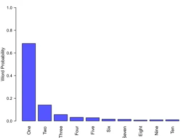
To create data for the learning model, we simulated noisy pairing of words and sets of objects, where the word frequencies approximate the naturalistic word probabilities in child-directed speech from CHILDES (MacWhinney, 2000). We used all English transcripts with children aged between 20 and 40 months to compute these probabilities. This distribution is shown in Figure 2. Note that all occurrences of number words were used to compute these probabilities, regardless of their annotated syntactic type. This was because examination of the data revealed many instances in which it is not clear if labeled pronoun usages actually have numerical content—e.g., “give me one” and “do you want one?” We therefore simply used the raw counts of number words. This provides a distribution of number words much like that observed cross-linguistically by Dehaene and Mehler (1992), but likely overestimates the probability of “one”. Noisy data that fits the generative assumptions of the model was created for the learner by pairing each set size with the correct word with probabilityα, and with a uniformly chosen word with probability 1− α.
11The second line is “α+(1−α)1
N” instead of just “α” since the correct word wican be generated either by producing
the correct word with probabilityα or by generating uniformly with probability 1 − α.
12It would be interesting to study the relationship of number learning to acquisition of other quantifiers, since they
One Tw
o
Three F
our Five Six
Se v en Eight Nine Ten W ord Probability 0.0 0.2 0.4 0.6 0.8 1.0
Figure 2. : Number word frequencies from CHILDES (MacWhinney 2000) used to simulate learn-ing data for the model.
Inference & Methods
The previous section established a formal probabilistic model which assigns any potential hypothesized numerical system L a probability, conditioning on some observed data consisting of sets and word-types. This probabilistic model defines the probability of a lambda expression, but does not say how one might find high-probability hypotheses or compute predicted behavioral pat-terns. To solve these problems, we use a general inference algorithm similar to the tree-substitution Markov-chain monte-carlo (MCMC) sampling used in the rational rules model.
This algorithm essentially performs a stochastic search through the space of hypotheses L. For each hypothesized lexicon L, a change is proposed to L by resampling one piece of a lambda expression in L according to a PCFG. The change is accepted with a certain probability such that in the limit, this process can be shown to generate samples from the posterior distribution P(L|
W, T,C). This process builds up hypotheses by making changes to small pieces of the hypothesis:
the entire hypothesis space need not be explicitly enumerated and tested. Although the hypothesis space is in principle, infinite the “good” hypotheses can be found by this technique since they will be high-probability, and this sampling procedure finds regions of high probability.
This process is not necessarily intended as an algorithmic theory for how children actually discover the correct lexicon (though see Ullman et al., 2010). Children’s actual discovery of the correct lexicon probably relies on numerous other cues and cognitive processes and likely does not progress through such a simple random search. Our model is intended as a computational level model (Marr, 1982), which aims to explain children’s behavior in terms of how an idealized statis-tical learner would behave. Our evaluation of the model will rely on seeing if our idealized model’s degree of belief in each lexicon is predictive of the correct behavioral pattern as data accumulates during development.
To ensure that we found the highest probability lexicons for each amount of data, we ran this process for one million MCMC steps, for varyingγ and amounts of data from 1 to 1000 pairs of sets,
words, and types. This number of MCMC steps was much more than was strictly necessary to find the high probability lexicons and children could search a much smaller effective space. Running MCMC for longer than necessary ensures that no unexpectedly good lexicons were missed during the search, allowing us to fully evaluate predictions of the model. In the MCMC run we analytically computed the expected log likelihood of a data point for each lexicon, rather than using simulated data sets. This allowed each lexicon to be efficiently evaluated on multiple amounts of data.
Ideally, we would be able to compute the exact posterior probability of P(L| W,T,C) for any lexicon L. However, Equation 3 only specifies something proportional to this probability. This is sufficient for the MCMC algorithm, and thus would be enough for any child engaging in a stochastic search through the space of hypotheses. However, to compute the model’s predicted distribution of responses, we used a form of selective model averaging (Madigan & Raftery, 1994; Hoeting, Madigan, Raftery, & Volinsky, 1999), looking at all hypotheses which had a posterior probability in the top 1000 for any amount of data during the MCMC runs. This resulted in approximately 11, 000 hypotheses. Solely for the purpose of computing P(L| W,T,C), these hypotheses were treated as a fixed, finite hypothesis space. This finite hypothesis space was also used to compute model predictions for variousγ and α. Because most hypotheses outside of the top 1000 are extremely low probability, this provides a close approximation to the true distribution P(L| W,T,C).
Results
We first show results for learning natural numbers from naturalistic data. After that, we apply the same model to other data sets.
Learning natural number
The precise learning pattern for the model depends somewhat on the parameter valuesα and γ. We first look at typical parameter values that give the empirically-demonstrated learning pattern, and then examine how robust the model is to changing these parameters.
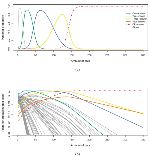
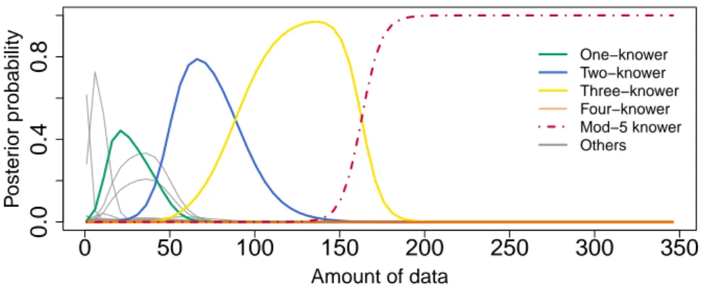
Figure 3 shows learning curves for the behavioral pattern exhibited by the model forα = 0.75 and logγ = −25. This plot shows the marginal probability of each type of behavior, meaning that each line represents the sum of the posterior probability all hypotheses that show a given type of behavior. For instance, the 2-knower line shows the sum of the posterior probability of all LOT expressions which map sets of size 1 to “one”, sets of size 2 to “two”, and everything else to undef . Intuitively, this marginal probability corresponds to the proportion of children who should look like subset- or CP-knowers at each point in time. This figure shows that the model exhibits the correct developmental pattern. The first gray line on the left represents many different hypotheses which are high probability in the prior—such as all sets map to the same word, or are undefined—and are quickly dispreferred. The model successively learns the meaning of “one”, then “two”, “three”, and finally transitioning to a CP-knower who knows the correct meaning of all number words. That is, with very little data the “best” hypothesis is one which looks like a 1-knower, and as more and more data is accumulated, the model transitions through subset-knowers. Eventually, the model accumulates enough evidence to justify the CP-knower lexicon that recursively defines all number words on the count list. At that point, the model exhibits a conceptual re-organization, changing to a hypothesis in which all number word meanings are defined recursively as in the CP-knower lexicon in Table 1.
The reason for the model’s developmental pattern is the fact that Bayes’ theorem implements a simple trade-off between complexity and fit to data: with little data, hypotheses are preferred
0 50 100 150 200 250 300 350 0.0 0.2 0.4 0.6 0.8 1.0 Amount of data P oster ior probability One−knower Two−knower Three−knower Four−knower CP−knower Others (a) 0 50 100 150 200 250 300 350 1e−26 1e−20 1e−14 1e−08 1e−02 Amount of data P oster
ior probability (log scale)
(b)
Figure 3. : Figure 3a shows marginal posteriors probability of exhibiting each type of behavior, as a function of amount of data. Figure 3b shows the same plot on a log y-axis demonstrating the large number of other numerical systems which are considered, but found to be unlikely given the data.
which are simple, even if they do not explain all of the data. The numerical systems which are learned earlier are simple, or higher prior probability in the LOT. In addition, the data the model receives follows word frequency distributions in CHILDES, in which the earlier number words are more frequent. This means that it is “better” for the model to explain the more frequent number words. Number word frequency falls off with the number word’s magnitude, meaning that, for instance, just knowing “one” is a better approximation than just knowing “two”: children become 1-knowers before they become 2-knowers. As the amount of data increases, increasingly complex hypotheses become justified. The CP-knower lexicon is most “complex,” but also optimally explains the data since it best predicts when each number word is most likely to be uttered.
The model prefers hypotheses which leave later number words as undef because it is better to predict undef than the wrong answer: in the model, each word has likelihood 1/N when the model predicts undef , but (1− α)/N when the model predicts incorrectly. This means that a hypothesis
likeλ S . (if (singleton? S) “one” undef ) is preferred in the likelihood to λ S . “one”. If the model did not employ this preference for non-commitment (undef ) over incorrect guesses, the 1-knower stage of the model would predict children say “one” to sets of all sizes. Thus, this assumption of the likelihood drives learners to avoid incorrectly guessing meanings for higher number words, preferring to not assign them any specific numerical meaning—a pattern observed in children.
Figure 3b shows the same results with a log y-axis, making clear that many other types of hypotheses are considered by the model and found to have low probability. Each gray line represents a different kind of knower-level behavior—for instance, there is a line for correctly learning “two” and not “one”, a line for thinking “two” is true of sets of size 1, and dozens of other behavioral patterns representing thousands of other LOT expressions. These are all given very low probability, showing the data that children plausibly receive is sufficient to rule out many other kinds of behavior. This is desirable behavior for the model because it shows that the model needs not have strong a priori knowledge of how the numerical system works. Many different kinds of functions could be built, considered by children, and ruled-out based on the observed data.
Table 2 shows a number of example hypotheses chosen by hand. This table lists each hy-pothesis’ behavioral pattern and log probability after 200 data points. The behavioral patterns show what sets of each size are mapped to13: for instance, “(1 2 U U U U U U U U)” means that sets of size 1 are mapped to “one” (“1”), sets of size 2 are mapped to “two” (“2”), and all other sets are mapped to undef (“U”). Thus, this behavior is consistent with a 2-knower. As this table makes clear, the MCMC algorithm used here searches a wide variety of LOT expressions. Most of these hypotheses have near-zero probability, indicating that the data are sufficient to rule out many bizarre and non-attested developmental patterns.
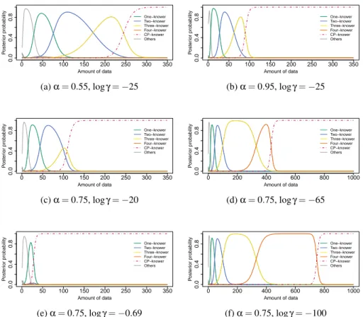
Figure 4 shows the behavioral pattern for different values of γ and α. Figures 4a and 4b demonstrate that the learning rate depends onα: when α is small, the model takes more data points to arrive at the correct grammar. Intuitively this is sensible becauseα controls the degree to which the model is penalized for an incorrect mapping from sets to words, meaning that whenα is small, the model takes more data to justify a jump to the more complex CP-knower hypothesis.
Figures 4c-4f demonstrate the behavior of the model asγ is changed. 4c and 4d show that a range of logγ that roughly shows the developmental pattern is from approximately −20 to −65, a range of forty-five in log space or over nineteen orders of magnitude in probability space. Even though we do not know the value ofγ, a large range of values show the observed developmental pattern.
Figures 4e and 4f show what happens as logγ is made even more extreme. The plot for γ = 1
2 (logγ = −0.69) corresponds to no additional penalty on recursive hypotheses. This shows a CP-transition too early—roughly after becoming a 1-knower. The reason for this may be clear form Figure 1: the CP-knower hypothesis is not much more complex than the 2-knower in terms of overall length, but does explain much more of the observed data. If logγ = −100, the model is strongly biased against recursive expressions and goes through a prolonged 4-knower stage. This curve also shows a long three-knower stage, which might be mitigated by including quadrupleton? as a primitive. In general, however, it will take increasing amounts of data to justify moving to the next knower-level because of the power-law distribution of number word occurrances—higher num-ber words are much less frequent. The duration of the last knower-level before the CP-transition, though, depends largely onγ.
Rank Log Posterior Beha vioral P attern LO T expression 1 -0.93 (1 2 3 4 5 6 7 8 9 10) λ S . (if (singleton? S ) “one” (ne xt (C (set-dif fer ence S (select S ))))) 2 -2.54 (1 2 3 4 5 6 7 8 9 10) λ S . (if (singleton? S ) “one” (ne xt (C (set-dif fer ence S (select (select S )))))) 3 -3.23 (1 2 3 4 5 6 7 8 9 10) λ S . (if (not (singleton? S )) (ne xt (C (set-dif fer ence S (select S )))) “one” ) 1604 -14.12 (1 2 3 U U U U U U U) λ S . (if (tripleton? S ) “thr ee” (if (doubleton? (union S S )) “one” (if (doubleton? S ) “two” U ))) 1423 -11.92 ( 1 2 3 U U U U U U U) λ S. (if (tripleton? S ) “thr ee” (if (singleton? S ) “one” (if (doubleton? S ) “two” U )))) 4763 -20.04 1 2 U U U U U U U U) λ S . (if (doubleton? (union S S )) “one” (if (doubleton? S ) “two” U )) 7739 -39.42 (1 U 3 U U U U U U U) λ S . (if (tripleton? S ) “thr ee” (if (singleton? S ) “one” U )) 7756 -44.68 (1 U U U U U U U U U) λ S . (if (singleton? S ) “one” U ) 7765 -49.29 (1 2 4 4 4 4 4 4 4 4) λ S . (if (doubleton? S ) “two” (if (singleton? S ) “one” “four” )) 9410 -61.12 (1 2 1 1 1 1 1 1 1 1) λ S . (if (not (not (doubleton? S ))) “two” “one” ) 9411 -61.12 (1 2 2 2 2 2 2 2 2 2) λ S . (if (not (not (singleton? S ))) “one” “two” ) 9636 -71.00 (1 2 7 1 1 1 1 1 1 1) λ S . (pr ev (pr ev (if (doubleton? S ) “four” (if (tripleton? S ) “nine” “thr ee” )))) 9686 -100.76 (1 3 3 3 3 3 3 3 3 3) λ S . (if (singleton? S ) “one” “thr ee” ) 9695 -103.65 (1 1 3 1 1 1 1 1 1 1) λ S . (if (tripleton? S ) (pr ev “four” ) “one” ) 9765 -126.01 (1 1 1 1 1 1 1 1 1 1) λ S . (ne xt (pr ev “one” )) 11126 -396.78 (2 U U U U U U U U U) λ S . (if (singleton? S ) “two” U ) 11210 -444.68 (2 U 2 2 2 2 2 2 2 2) λ S . (if (not (doubleton? S )) “two” U ) T able 2: : Se v eral hand-selected example h ypotheses at 200 data points.
0 50 100 150 200 250 300 350 0.0 0.4 0.8 Amount of data P oster ior probability One−knower Two−knower Three−knower Four−knower CP−knower Others (a)α = 0.55, logγ = −25 0 50 100 150 200 250 300 350 0.0 0.4 0.8 Amount of data P oster ior probability One−knower Two−knower Three−knower Four−knower CP−knower Others (b)α = 0.95, logγ = −25 0 50 100 150 200 250 300 350 0.0 0.4 0.8 Amount of data P oster ior probability One−knower Two−knower Three−knower Four−knower CP−knower Others (c)α = 0.75, logγ = −20 0 200 400 600 800 1000 0.0 0.4 0.8 Amount of data P oster ior probability One−knower Two−knower Three−knower Four−knower CP−knower Others (d)α = 0.75, logγ = −65 0 50 100 150 200 250 300 350 0.0 0.4 0.8 Amount of data P oster ior probability One−knower Two−knower Three−knower Four−knower CP−knower Others (e)α = 0.75, logγ = −0.69 0 200 400 600 800 1000 0.0 0.4 0.8 Amount of data P oster ior probability One−knower Two−knower Three−knower Four−knower CP−knower Others (f)α = 0.75, logγ = −100
Figure 4. : Behavioral patterns for different values ofα and γ. Note that the X-axis scale is different for 4d and 4f.
These results show that the dependence of the model on the parameters is fairly intuitive, and the general pattern of knower-level stages preceding CP-transition is a robust property of this model. Because γ is a free parameter, the model is not capable of predicting or explaining the precise location of the CP-transition. However, these results show that the behavior of the model is not extremely sensitive to the parameters: there is no parameter setting, for instance, that will make the model learn low-ranked hypotheses in Table 2. This means that the model can explain why children learn the correct numerical system instead of any other possible expression which can be expressed in the LOT.
Next, we show that the model is capable of learning other systems of knowledge when given the appropriate data.
Learning singular/plural
An example singular/plural system is shown in Table 1. Such a system differs from subset-knower systems in that all number words greater than “one” are mapped to “two”. It also differs from the CP-knower system in that it uses no recursion. To test learning for singular/plural cognitive representations, the model was provided with the same data as in the natural number case, but sets with one element were labeled with “one” and sets with two or more elements were labeled with
5 10 15 20 0.0 0.4 0.8 Amount of data P oster ior probability All−singular All−plural Correct Others
Figure 5. : Learning results for a singular/plural system.
“two”. Here, “one” and “two” are just convenient names for our purposes—one could equivalently
consider the labels to be singular and plural morphology.
As Figure 5 shows, this conceptual system is easily learnable within this framework. Early on in learning this distinction, even simpler hypotheses than singular/plural are considered: λ S .
“one” andλ S . “two”. These hypotheses are almost trivial, but correspond to learners who initially
do not distinguish between singular and plural markings—a simple, but developmentally-attested pattern (Barner, Thalwitz, Wood, Yang, & Carey, 2007). Here,λ S . “one” is higher probability thanλ S . “two” because sets of size 1 are more frequent in the input data. Eventually, the model learns the correct hypothesis, corresponding to the singular/plural hypothesis shown in Figure 1. This distinction is learned very quickly by the model compared to the number hypotheses, matching the fact that children learn the singular/plural distinction relatively young, by about 24 months (Kouider, Halberda, Wood, & Carey, 2006). These results show one way that natural number is not merely “built in”: when given the different kind of data—the kind that children presumably receive in learning singular/plural morphology—the model infers a singular/plural system of knowledge.
Learning Mod-N systems
Mod-N systems are interesting in part because they correspond to an inductive leap consistent with the correct meanings for early number words. Additionally, children do learn conceptual sys-tems with Mod-N-like structures. Many measure of time—for instance, days of the week, months of the year, hours of the day—are modular. In numerical systems, children eventually learn the dis-tinction between even and odd numbers, as well as concepts like “multiples of ten.” Rips, Asmuth, and Bloomfield (2008) even report anecdotal evidence from Hartnett (1991) of a child arriving at a Mod-1,000,100 system for natural number meanings14.
14They quote,
D.S.: The numbers only go to million and ninety-nine. Experimenter: What happens after million and ninety-nine? D.S.: You go back to zero.
E: I start all over again? So, the numbers do have an end? Or do the numbers go on and on?
When the model is given natural number data Mod-N systems are given low probability because of their complexity and inability to explain the data. A Mod-N system makes the wrong predictions about what number words should be used for sets larger than size N. As Table 1 shows, modular systems are also considerably more complex than a CP-knower lexicon, meaning that they will be dispreferred even for huge N, where presumably children have not received enough data. This means that Mod-N systems are doubly dispreferred when the learner observes natural number data.
To test whether the model could learn a Mod-N system when the data support it, data was generated by using the same distribution of set sizes as for learning natural number, but sets were labeled according to a Mod-5 system. This means that the data presented to the learner was identical for “one” through “five”, but sets of size 6 were paired with “one”, sets of size 7 were paired with
“two”, etc. As Figure 6 shows, the model is capable of learning from this data, and arriving at the
correct Mod-5 system15. Interestingly, the Mod-learner shows similar developmental patterns to the natural number learners, progressing through the correct sequence of subset-knower stages before making the Mod-5-CP-transition. This results from the fact that the data for the Mod system is very similar to the natural number data for the lower and more frequent set sizes. In addition, since both models use the same representational language, they have the same inductive biases, and thus both prefer the “simpler” subset-knower lexicons initially. A main difference is that hypotheses other than the subset-knowers do well early on with Mod-5 data. For instance, a hypothesis which maps all sets to “one” has higher probability than in learning number because “one” is used for more than one set size.
The ability of the model to learn Mod-5 systems demonstrates that the natural numbers are no more “built-in” to this model than modular-systems: given the right data, the model will learn either. As far as we know, there is no other computational model capable of arriving at these types of distinct, rule-based generalizations.
Discussion
We have presented a computational model which is capable of learning a recursive numerical system by doing statistical inference over a structured language of thought. We have shown that this model is capable of learning number concepts, in a way similar to children, as well as other types of conceptual systems children eventually acquire. Our model has aimed to clarify the conceptual re-sources that may be necessary for number acquisition and what inductive pressures may lead to the CP-transition. This work was motivated in part by an argument that Carey’s formulation of boot-strapping actually presupposes natural numbers, since children would have to know the structure of natural numbers in order to avoid other logically-plausible generalizations of the first few
num-ninety-nine.
E: . . .you start all over again.
D.S.: Yeah, you go zero, one, two, three, four—all the way up to million and ninety-nine, and then you start all over again.
E: How about if I tell you that there is a number after that? A million one hundred.
D.S.: Well, I wish there was a million and one hundred, but there isnt.
15Because of the complexity of the Mod-5 knower, special proposals to the MCMC algorithm were used which
0 50 100 150 200 250 300 350 0.0 0.4 0.8 Amount of data P oster ior probability One−knower Two−knower Three−knower Four−knower Mod−5 knower Others
Figure 6. : Learning results for a Mod-5 system.
ber word meanings. In particular, that there are logically possible modular number systems which cannot be ruled out given only a few number word meanings (Rips et al., 2006; Rips, Asmuth, & Bloomfield, 2008; Rips, Bloomfield, & Asmuth, 2008). Our model directly addresses one type of modular system along these lines: in our version of a Mod-N knower, sets of size k are mapped to the k mod Nth number word. We have shown that these circular systems of meaning are simply less likely hypotheses for learners. The model therefore demonstrates how learners might avoid some logically possible generalizations from data, and furthermore demonstrates that dramatic in-ductive leaps like the CP-transition should be expected for ideal learners. This provides a “proof of concept” for bootstrapping.
This work leaves open the question of whether the model learns the true concept of natural number. This is a subtle issue because it is unclear what it means to have this concept (though see Leslie et al., 2008). Does it require knowledge that there are an infinitity of number concepts, or number words? What facts about numbers must be explicitly represented, and which can be implicitly represented? The model we present learns natural number concepts in the sense that it relates an infinite number of set-theoretic concepts to a potentially infinite list of number words, using only finite evidence. However, the present work does not directly address what may be an equally-interesting inductive problem relevant to a full natural number concept: how children learn that next always yeilds a new number word. If it was the case that next at some point yeilded a previous number word—perhaps (next fifty) is equal to “one”—then learners would again face a problem of a modular number system16. It is likely that similar methods to those that we use to solve the inductive problem of mapping words to functions could also be applied to learn that next always maps to a new word. It would be surprising if next mapped to a new word for 50 examples, but not for the 51st. Thus, the most concise generalization from such finite evidence is likely that
next never maps to an old linguistic symbol17.
The model we have developed also suggests a number of possible hypotheses for how
nu-16It is not clear to us which form of modular system Rips, Asmuth, and Bloomfield intended as the prototypical
inductive problem in their papers, although one of the authors in an anonymous review suggested it is this latter form.
17In some programming languages, such as scheme, there is even a single primitive function gensym, for creating new
merical acquisition may progress:
The CP transition may result from bootstrapping in a general representation language.
This work was motivated in large part by the critique of bootstrapping put forth by Rips, Asmuth, and Bloomfield (Rips et al., 2006; Rips, Asmuth, & Bloomfield, 2008; Rips, Bloomfield, & Asmuth, 2008). They argued that bootstrapping presupposed a system isomorphic to natural numbers; indeed, it is difficult to imagine a computational system which could not be construed as “building in” natural numbers. Even the most basic syntactic formalisms—for instance, finite-state grammars—can create a discrete infinity of expressions which are isomorphic to natural numbers. This is true in our LOT: for instance the LOT can generate expressions like (next x), (next (next x)), (next (next (next x))), etc.
However, dismissing the model as “building in” natural number would miss several important points. First, there is a difference between representations which could be interpreted externally as iosmorphic to natural numbers, and those which play the role internally as natural number repre-sentations. An outside observer could interpret LOT expressions as isomorphic to natural numbers, even though they do not play the role of natural numbers in the computational system. We have been precise that the space of number meanings we consider are those which map sets to words: the only things with numerical content in our formalization are functions which take a set as input and return a number word. Among the objects which have numerical content, we did not assume a successor function: none of the conceptual primitives take a function mapping sets of size N to the N’th word, and give you back a function mapping sets of size N + 1 to the N + 1’st word. Instead, the correct successor function is embodied as a recursive function on sets, and is only one of the potentially learnable hypotheses for the model. Our model therefore demonstrates that a bootstrapping theory is not inherently incoherent or circular, and can be both formalized and implemented.
However, our version of bootstrapping is somewhat different from Carey’s original formu-lation. The model bootstraps in the sense that it recursively defines the meaning for each number word in terms of the previous number word. This is representational change much like Carey’s theory since the CP-knower uses primitives not used by subset knowers, and in the CP-transition, the computations that support early number word meanings are fundamentally revised. However, unlike Carey’s proposal, this bootstrapping is not driven by an analogy to the first several number word meanings. Instead, the bootstrapping occurs because at a certain point learners receive more evidence than can be explained by subset-knowers. According to the model, children who receive evidence only about the first three number words would never make the CP-transition because a simpler 3-knower hypothesis could better explain all of their observed data. A distinct alternative is Carey’s theory that children make the CP-transition via analogy, looking at their early number word meanings and noticing a correspondence between set size and the count list. Such a theory might predict a CP-transition even when the learner’s data only contains the lowest number words, although it is unclear what force would drive conceptual change if all data could be explained by a simpler system18.
18These two alternatives could be experimentally distinguished by manipulating the type of evidence 3-knowers
re-ceive. While it might not be ethical to deprive 3-knowers of data about larger number words, analogy theories may predict no effect of additional data about larger cardinalities, while our implementation of bootstrapping as statistical inference does.