Analysis of mixing data relevant to wire wrapped fuel assembly thermal-hydraulic design

yCLEAR EN&6NJEA

SALA

NY

02

COO-2245-12 Topical-Report

MITNE-1 65

NUCLEAR

ENCNEERING

READING

ROOM

-

M.I.T.

ANALYSIS OF MIXING DATA RELEVANT

TO WIRE WRAPPED FUEL ASSEMBLY

THERMAL-HYDRAULIC DESIGN

E. U. Khan

N. E. Todreas

W. M. Rohsenow

A A. Sonin

September 1974

Departments of Mechanical Engineering and Nuclear Engineering

Massachusetts Institute of Technology

Cambridge, Massachusetts 02139

AEC Research and Development

Contract AT(1 1-1)-2245

U.S. Atomic Energy Commission

fiL

§2

I,

ANALYSIS OF MIXING DATA RELEVANT TO

WIRE-WRAPPED FUEL ASSEMBLY

THERMAL-HYDRAULIC DESIGN by

E. U. Khan

N. E. Todreas

W. M. Rohsenow

A. A. Sonin

Massachusetts Institute of Technology

TABLE OF CONTENTS

ABSTRACT 1. INTRODUCTION

2. Theoretical Background

3. Results of Data Analysis

3.1 Overview

3.2 Comparison of Heated Pin, Hot Water Injection

and Salt Injection Experiment 3.3 Reynolds Number Effect

3.4 Bundle Size Effect

4. 4.1 Application of ENERGY code calculations to a 217-pin FFTF Bundle at Full Power

5. 5.1 Proposed Experiments (to fill in data gaps and enhance confidence in predictions)

5.2 Experiment I

5.3 Experiment II

6. Tables and Figures for Sections 1 through 5 and Nomenclature

7. Appendix

7.1 Analysis of Data and ENERGY Calibration

7.2 Definitions of mixing mechanisms 7.3 Tables and Figures for Appendix

ABSTRACT

In this report analysis of recent experimental

data is presented using the ENERGY code. A comparison

of the accuracy of three types of experiments is also

presented along with a discussion of uncertainties in

utilizing this data for various code calibration

pur-poses. The existence of internal swirl is discussed.

The two empirical coefficients in ENERGY are determined

from the data within a certain range of accuracy. This

range is dictated to a large extent by the accuracy of

the experiments and to a smaller extent by the ability

of the code to utilize all sets of data in each

experiment.

The effect of geometry and bundle size on mixing

and swirl flow is discussed. A realistic estimate of

the degree of accuracy within which we can predict

temperature distribution within the bundle and along

the duct of a 217-pin wire wrapped fuel assembly of

an LMFBR is presented.

Gaps in data which need to be filled in to enhance

our confidence in predicting coolant temperature

dis-tributions in a 217-pin LMFBR fuel bundle, are given.

A brief description of two experiments that would fill

would be very useful for both fuel and poison assembly

mixing studies is described. Conclusions drawn from

Acknowledgement

The authors are grateful to Dr. L. Wolf for

discussions and for bringing to our notice

reports from Karlshrue. We also would like to thank

Mr. Y. Chen, Mr. A. Hanson and Mr. T. Eaton for their

comments in reviewing this report. In addition we

would like to thank Dr. J. J. Lorenz of Argonne National

1. INTRODUCTION

In the design of a wire wrapped Liquid Metal Fast

Breeder Reactor (LMFBR) fuel assembly,coolant mixing caused by wire wraps is the most significant mode of itt'gy

re'ds-(1 ,2)*

tribution ' . At the high Reynolds number range of steady

state operation of a typical LMFBR energy transport by

conduction plays a secondary role only to energy transport

by wire wrap mixing.

The maximum burnup (Mwd/T) for current LMFBR designs

is very sensitive to the peak coolant temperature in the hot

channel3, which in turn could depend, to a large extent, on interchannel mixing fates. In addition, the fuel assembly

housing bowing is also of special concern. Bowing of the

hexagonal housing is caused by differential thermal expansion.

It is greatly enhanced by radiation induced stainless steel

swelling in a fast spectrum and the temperature dependence of

this induced swelling. Thus realistic predictions of assembly

temperature distribution could have important effects on the

flow housing design considerations. At present a purely

theo-retical analysis is not adequate to establish the extent of

mixing caused by wire wraps in LMFBR assemblies. In order to

reduce the uncertainty in predicting mixing rates caused by

wire wraps (also known as flow sweeping - see Section 7.2

and Ref. 2 for a detailed description of various other modes

of energy transport) many different types of experiments

have been performed. Some of these experiments, in addition

to providing data from which mixing-coefficients can be

determined for use in computer programs, provide useful

information on flow and pressure distribution in the rod

bundle.

The three types of experiments that are most

fre-quently used for determining wire-wrap mixing in a rod

bundle can be classified according to their boundary

con-ditions.

1) Continuous injection of an electrolyte salt solution at a

point in the bundle. Electrical conductivity measurements

at various points in the rod bundle can give an estimate

of the amount of salt transported by mixing. From this a

mixing coefficient can be derived.

2) Continuous local injection of heated coolant. Temperature

measurement in the three dimensional bundle matrix will

yield a mixing coefficient with appropriate data analysis. 3) Employment of one, several, or a complete array of heated

pins.4 By measuring temperature distributions in the bundle, one can derive a mixing coefficient.

The mixing coefficient one would like to derive

from these experiments should solely represent the contribution

of wire-wraps in promoting energy transport from one point to

other modes of energy transport co-exist (e.g. diversion

cross-flow, flow scattering, energy transfer by turbulence)

although their magnitudes may be considerably smaller than

the wire wrap sweeping effect. It is often not possible to

separate (except for thermal conduction) the individual

contributions of the mixing mechanisms, from these experiments,

to a good degree of accuracy. This is one of the reasons why

computer programs like ENERGY combine all the mixing

mecha-nisms into one lumped mixing coefficient which is empirically

determined. Other computer programs make an effort to dIetermine

the individual contributions of the wire-wrap, sweeping,

diversion cross-flow and turbulence energy exchange and

linearly add them. Linear addition of these effects is

questionable. However, since the flow sweeping by wire wraps

so completely dominates the mixing process, errors in either

neglecting or linearly adding the effect of other mixing

mechanisms are expected to be small. In addition to the

ex-periments mentioned before, experimenters have used several techniques to measure axial and circumferential velocities in wire wrapped rod bundles. One of these is the use of Laser

Doppler Velocimeter to determine velocity and turbulent

intensity.

In this respect analysis of recent experimental data

is presented using the ENERGY code. A comparison of the

accuracy of three types of experiments is also presented along

various code calibration purposes. The existence of internal

swirl is discussed. The two empirical coefficients in ENERGY

are determined from the data within a certain range of

accuracy. This range is dictated to a large extent by the

accuracy of the experiments and to a smaller extent by the

ability of the code to utilize all sets of data in each

experiment. The effect of geometry and bundle size on mixing

and.swirl flow is discussed. A realistic estimate of the

degree of accuracy within which we can predict temperature

distribution within the bundle and along the duct of a

217-pin wire wrapped fuel assembly of an LMFBR is presented.

Gaps in data, which need to be filled in, to enhance our

confidence in predicting coolant temperature distributions

in a 217-pin LMFBR fuel bundle, are given. A brief description

of two experiments that would fill these data gaps is presented.

A novel idea for an experiment which would be very useful for

both fuel and poison assemblies mixing studies is described.

It is necessary to point out that the conclusions

drawn from this study regarding flow distributions within the

fuel assembly, internal swirl, bundle size effects, effect of

geometry on mixing and swirl are quite general in nature. The

code used to obtain these conclusions is the ENERGY code.

However, the results and conclusions are expected to be

2. Theoretical Background

The ENERGY1 computer program models the periodic

sweep flow through rod gaps as an enhanced effective eddy

diffusivity. The model subdivides the fuel assembly into

two predominant regions. In the central region the enhanced

effective eddy diffusivity is responsible for energy transport

in the transverse directions. Near the duct wall, flow is

unidirectional and parallel to the duct wall. Energy transport

can occur both by diffusion and by convection, although it

has been found that the eneray transport by convection (swirl

flow) predominates. ENERGY models the heat aeneration in the

fuel rods as a volumetric heat source in the fluid. Until more

data is available ENERGY uses two options for flow split.

1) Hydraulic diameter flow split, 2) uniform velocity in the

entire bundle. Each set of data was analyzed by taking two

splits into consideration. The available data yields some

useful information on this flow split, as is shown later.

The ENERGY code requires as input two empirical

constants c* and C All the mixing effects (e.g. turbulent

exchange, diversion cross-flow, flow sweep due to wire wraps)

are lumped into H = [eH/(Vde)]. It should however be noted that the effect of wire wrap for the current fuel assembly

design almost completely dominates other effects included in

E*.

H 1asts the swirl flo in the gap retween is

and wall to the average axial bundle velocity (C = Vg/V).

It is necessary to note that C1 is assumed to be uniform

around the bundle and represents the average circumferential swirl velocity in the gap between rod and wall. The three

types of experiments, namely, electrolyte salt injection, hot

water injection experiment, and heated pins, are used to

determine c* and C1. Based on physical insight and inspection

of the fundamental energy balance equation we can determine

that c* and C are dependent on the following parameters,

H

1

e

H

C1 = f(h/d, p/d, Re, Pr) (2)

Since these experiments have been performed for fuel assemblies

of different geometries and at various Reynolds numbers it is

possible to determine these functional relationships for E*

H

The heated pin experiments provide a boundary condition which represents the actual LMFBR fuel assembly assembly heat

transfer boundary condition. The parameters E* and C1 in

ENERGY are varied until coolant temperatures predicted by the

code match the experimentally measured temperatures.It was

found that c* and C can be found independently by matching

the central region and wall region temperature maps respectively.

Apparently, swirl flow effects, fortunately, do not appear to

be determined from the data in the inner region and C1 from the data on the wall region.

In order to show that both the salt injection and hot

water injection experiments would also yield a mixing

co-efficient which can directly be used in the ENERGY code for

LMFBR fuel assembly temperature calculations, it is necessary

to realize that e* predominantly represents the wire sweep

flow mixing effect. Thus the mixing coefficients determined

from equations (3) and (4) below need not be modified (as is

normally done in literature when mass eddy diffusivities are

converted to heat eddy diffusivities or vice versa) in any

manner for use in ENERGY.

The equations governing salt diffusion in salt injection

experiments and heat diffusion in hot water injection

experi-ments along with injection boundary conditions are given below

(note: we may only concern ourselves with the steady state

equation), Hot Water. DT* _ 1 H + 1 ) V2T* (3) Injection' Dt Re y Pr T - TCOLD whenz=,T*=where T* T -T HOT COLD

Water is generally used as the working fluid. One

finds -- >> g

P

fr

Salt DC* _ l D + 1 ) V2C* (4)

Injection Dt Re y Sc

when z = 0, C* = 1 where C* = and C₀ inlet concentration

For all tracers utilized in wire wrap studies

inde-D

1

pendent of the particular tracer - >>L. For reasons

discussed before one expects e* = c*

3. RESULTS OF DATA ANALYSIS AND ENERGY CALIBRATION

3.1

Overview

Fig. 3.1 shows a comparison of the theoretical

(hydraulic diameter including the effect of wire-wrap presence)

flow split and experimentally observed flow split for the wall channels of wire-wrap bundles ranging in size from 7

to 217 pins. The theoretical flow split was obtained by

(a) completely neglecting geometrical tolerance, and (b)

allowing for geometrical tolerance. In reality, geometrical

tolerance effect exists and must be taken into account.

Following the method given by Hanson in Ref. 4 (appendix)

if T is the diametrical tolerance across the flats of a bundle,

a fraction F of this would be accomodated within the bundle

and a fraction (1 - F) in the wall region. Then the pitch, P, of the wire wrapped bundle must be increased by AP due to

the "looseness" caused by geometrical tolerance, where

AP = TF/(/3.NRINGS)

The gap between the wire and the wall is given by

AR = (1 - F)

The two extreme cases for tolerance distribution are

Case I: F = 0 AP = 0 AR = T/2

Case II: F = 1 AP = T/(/3.NRINGS) AR = 0

The effect of these two extreme cases on flow split

bundle which has a diametrical tolerance of 0.0195 inches in

a duct with a distance across the hexagonal flats of 2.560 in.

In most bundles it is expected that Case II will

exist where all the tolerance is accomodated within the bundle.

Observation of the (Ref. 4) M.I.T. bundle agrees with this

suggestion as the pins were observed to contact the duct faces

when the bundle was assembled. This was also observed in the

AI 217 pin bundle (Ref. 30). Wherever there is a doubt as

to which of the two limiting cases exists within a bundle, we

have shown the two limits of flow splits for wall channel

corresponding to the two cases.

It is interesting to note that for the 7-pin bundle

it was possible to predict both the wall channel and inner

channel flow splits (see Section 7) accurately. As the bundle

size increased there appears to be a divergence between the

theoretical predictions and experimentally observed data on

a similar geometry. Allowing for the experimental predictions

to have an associated error bar, it still appears that the

theoretical flow split predicts higher axial velocities in

the wall channels (and lower axial velocities in central and

corner channels) than experimentally observed. If the divergence

in the theoretical and experimental curves is in fact real then

a correction factor on hydraulic diameter alone would not bring

the two curves together. A bundle size effect exists in that

case. If a bundle size effect exists it could be only due to

a change in the basic flow field in going from a 7-pin to a

Until this is fully resolved one needs to take into

account the flow split effect while analyzing other data and

in predicting temperatures for the full size bundle at power

conditions. The ENERGY analysis of data (Section 7) takes

into account a flow split effect in calibrating the two

constants e* and C 1

H

1

A thorough analysis of each set of data described in

Section 7 was made using the ENERGY code. It was necessary

to completely understand the experimental techniques used to

obtain the specific set of data including tolerance on

geo-metry, accuracy of measurements and the fraction of total

data, in any one experiment, that is useful for calibration

purposes. In addition the ENERGY code has certain inherent

assumptions built into it. Our ability to analyze a certain

set of experimental data was superimposed upon the expected accuracy of the data to determine a realistic error bar on

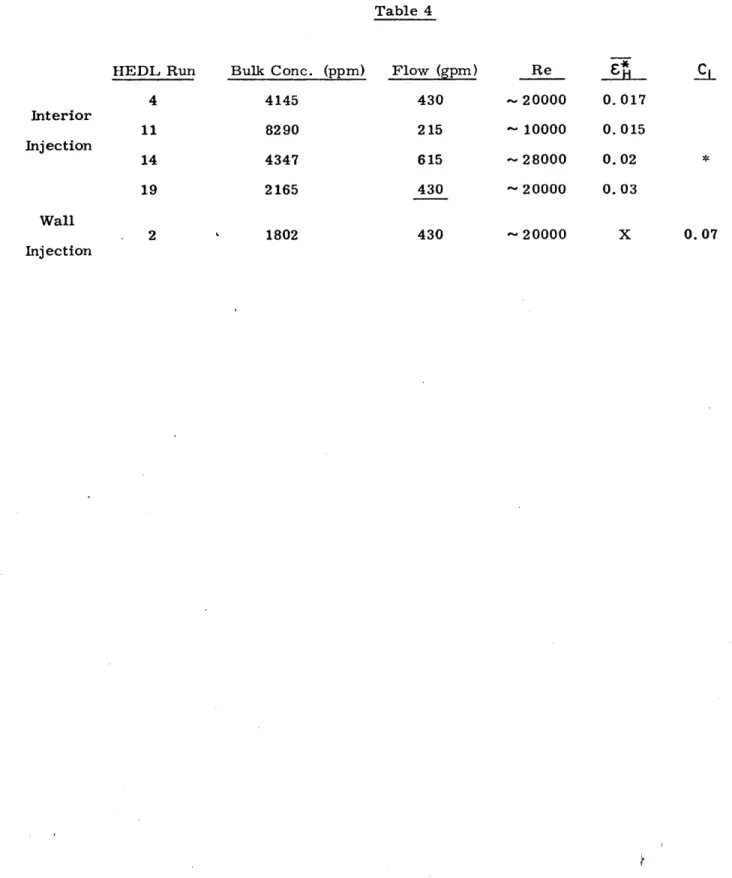
E* and C For example, for the FFTF geometry the HEDL tests

H

le

yield an s* from 0.015 to 0.03, whereas the O.R.N.L. tests

H

give an s* from 0.028 to 0.048. Considering the fact that

H

the HEDL data could only be used after the first twelve inches

from the inlet;that mass balances changed continuously from

inlet to exit; that there appeared to be an effect of injection

concentration; that two point measurements in the same channel

gave results up to 50% different; that the boundary condition

of salt injection is not a prototype boundary condition; one

heated data. However, the O.R.N.L. experiments were on a much

smaller bundle and rod bowing and bundle helixing at large

power input rates were observed. Since ENERGY could predict

many sets of data for various power skews with almost a single

value of e*

_H

19 pin experiments. Therefore the range of

E

H

(for p/d ,. 1.24,

h/d

to 0.048 with a weighted mean around 0.04. As will be seen

later (Section 4) such a large range in E only slightly

affects the exit temperature distribution and the maximum

exit temperature of a 217 pin FFTF bundle at full power.

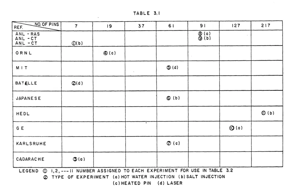
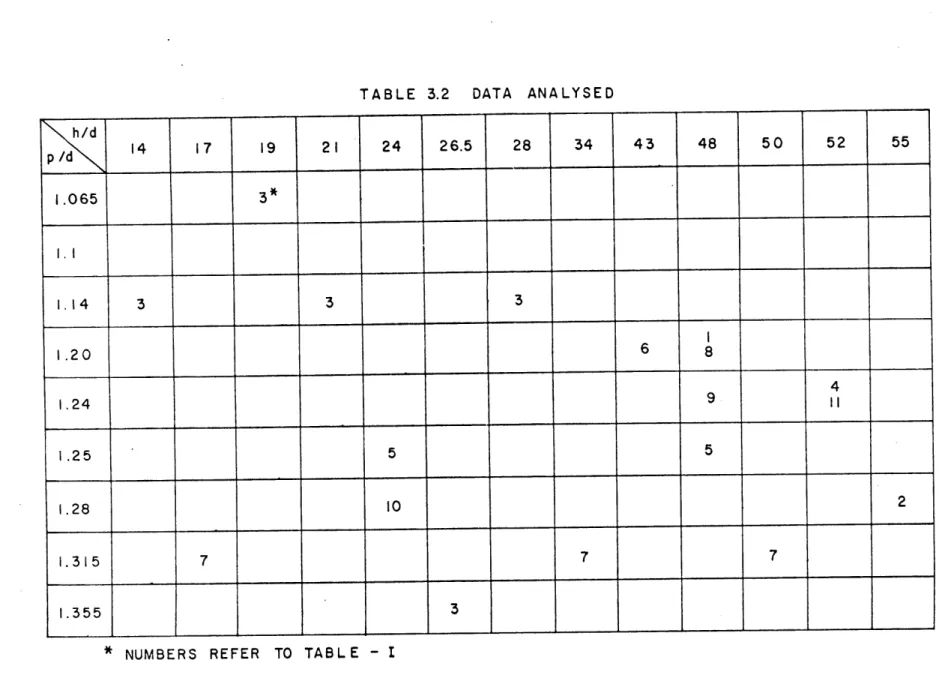
Tables 3.1 and 3.2 show the fuel-assembly data

ana-lyzed. Table 3.1 lists the data based on bundle size and

experimental techniques and Table 3.2 based on the significant geometrical characteristics. Only data relevant to fuel assembly

calculations was considered for analysis and only the data for

which all required details were available was analyzed. Although

the standard fuel assembly geometry is d \, 1/4", h/d \, 50, p/d -, 1.25, the data analyzed covers a reasonably wide range

about the standard fuel assembly design in order to permit

thermal-hydraulic optimization studies. No data on poison and

blanket assemblies was analyzed as this is not the present goal.

Fig. 3.2 shows that the variation of E* vs 1/(h/d)

H

is linear in the range of interest. As the wire wrap nitch is

increased

(d/h

wire-wrap. Only the natural turbulence effect would be

contributing to e* in that case. Fig. 3.3 is a cross-plot

H

of Fig. 3.2. It shows that the

E*

H

in between p/d of 1.2 and 1.3. Fig. 3.4 shows the variation

of C₁ (= Vi /7) vs d/h. There seems to be better agreement in

data at d/h n 0.02 (h/d ^ 50) than at larger values of d/h.

The only available data for large values of d/h (d/h > 0.02)

are the SKOK (Ref. 8) and M.I.T (3) data.

For practical use the recommended value of c is the

H

value read from Figs. 3.2 or 3.3 with approximately a 4-30% (of

s*)

in Fig. 3.2 is 0.025 to 0.048. Wherever the range is not

shown the above mentioned range in e* may be used. For C the

H

1

range shown in Fig. 3.4 must be used.

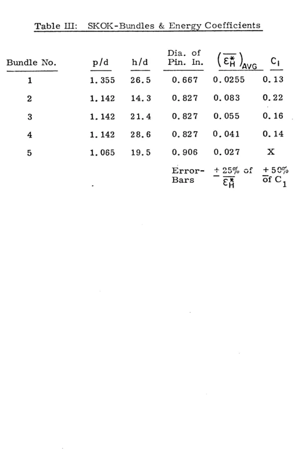
The analysis of data of Ref. 8 is described in Section

7 and Table III. Since only data over one axial wire wrap

pitch is given in Ref.8, our confidence level in analyzing it

is not good. The values of C1 obtained from the data of Ref. 8

required many assumptions. It appeared that C1 so obtained was

underestimated. Thus the SKOK data is shown as a lower limit

on C The M.I.T. results on the other hand appear to overpredict

C . This is because only one value of transverse velocity in the gap between rod and wall was measured. If the flow field is

turbulent, the average gap velocity could be as much as 20%

lower than the point velocity measured. Superimposed upon this

velocity profile effect is an independent error bar in the

range 12 to 14%. The value of C1 lies between the limits shown

The value of C for the FFTF geometry lies somewhere

between 0.07 from the HEDL data to 0.12 from O.R.N.L.9 and

M.I.T. data. Discussions of bundle size effect are delayed

until later. However the effect of this range of C1 on the

duct temperature gradient (Section 4) does not appear to be

very significant.

The calibration of ENERGY described above should hold

for the p/d and h/d ratios considered. In addition all of the

data (except SKOK data for which ENERGY calibration is not

expected to be good) used was for rod diameters close to 0.25

in. Rod diameters in a range close to this should present no

significant effect on e*. This limitation is imposed as a

precautionary measure (see Ref. 26; calibration of THI-3D

also imposes this limitation) since data with other rod diameters

have not been analyzed.

3.2 Comparison of Heated Pin, Hot Water Injection and Salt Injection Experiments

Our analysis of the various types of data showed that

the heated pin experiments are probably the most reliable,

provided care is taken in designing the temperature sensors

and the heated rods. The discussion to follow compares heated

pin experiments with non-heated pin experiments (salt and hot

water injection included). The Laser Doppler Velocimeter

ex-periments are not discussed since they can at present only be

used for wall channels where they can supplement the results

The major problem with the two non-heated experiments

(apart from a different boundary condition than the prototype)

is that an injector must be introduced into the main flow

stream. Local perturbations of the bulk flow can affect the

measurements many inches downstream of the injection point.

Three factors that are extremely important in obtaining reliable

reproducible results with any injection device are the injector

design, injector position and injection flow rate1 2'1 9

Considerable effort has been devoted by Lorenz19 and Pederson1 2

in testing various injector designs. Their results show a

centrally located injector with injection velocities close to

the local mainstream velocity should give reliable results for

wall channels. An extension of a similar detailed study 24 for

centrally located injector is required for central channels.

The HEDL inlet perturbation effects were found to last from

6 in to 9 in. The flow drift of two channels (see Section 7) has been interpreted by investigators as an internal swirl

flow. ENERGY analysis shows that this drift is an inlet

per-turbation effect. A similar inlet perper-turbation effect was found

by examining, level by level, the GE-127 pin2 2 hot water injec-tion data. The inlet perturbainjec-tion in this case is an extremely

small internal swirl flow which dies off after about 12-18 in.

Every size of bundle tested needs to have a detailed

injection study made similar to that in Refs. 12 and 19,

espe-cially for wall channels. The state of our understanding of

that an injection scheme tested for a small bundle cannot be

used for a large bundle with a great deal of confidence. Thus

until a complete knowledge of the local flow fields within

subchannels of a wire wrapped bundle is available each bundle

would require related injector development work.

The tracer detection by wall thermocouples (for hot

water injection) and wall conductivity probes is a localized

point measurement not suitable for lumped subchannel analysis

computer programs. The isokinetic sampling technique 6, however,

along with conductivity probes (or thermocouples) located near

or at the center of the subchannel9,13 can yield more useful

results. Although wall thermocouples can be designed22 carefully,

a steep temperature gradient between wall and the center of

the subchannels could aive misleading results. The M.I.T.

experiments27 use a variable injection position and fixed

detection probes at the outlet of the bundle. These probes

are located at the center of the subchannels. The tracer

detection in non-heated experiments can, therefore, be

care-fully designed to give reliable results. The mass balance (in

salt-injection experiments) and energy balance (in hot water

injection experiments) should be as good as the energy balance

in heated pin experiments 9. To date poor mass balances23 and

energy balance1 2 for central injection have been obtained. Heated pin experiments (Refs. 9, 15) have yielded energy

bal-ance within 3-5% as compared to 13-35%23 for non-heated pin

The isokinetic sampling technique does not appear to

suffer from the same major drawbacks as the others but a

possible source of error in this technique is discussed below.

Using the isokinetic sampling technique the differential

static pressure between a subchannel and another reference

subchannel at the exit plane to the test section is measured

under the undisturbed conditions. Then an extraction device

is placed at the measuring plane and flow withdrawn until

the previous APref. between the subchannel and the reference

subchannel is obtained. It is then assumed that the original

flow split is re-established and the "proper flow" flow split

is being sampled 6. The problem with the technique is that

re-establishing the previous APref. between the subchannel and

reference subchannel is necessary but not sufficient to ensure

that the original flow split is established. This is because

the pressure difference between the subchannel in question and

subchannels other than the reference may not be the same as

before even though APref. has been re-established. Fig. 3.5

shows a comparison of isokinetic sampling data on nearly similar

6

19

geometries in a 7-pin and in a 91-pin experiment. Although wire orientations are different for the two cases the difference

in results cannot be explained by wire-orientation effect alone

since wire orientation C lies in between A and B but the

corres-ponding curve for C/C does not.

It could possibly be a bundle size effect. If the latter

is ruled out (at present the latter cannot be ruled out) then

experiments are required to test fully the reliability of

the isokinetic sampling method.

The most useful portion of the data generated by

salt and hot water injection experiments is produced in the

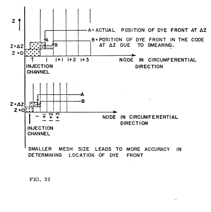
first twelve to fifteen inches axially. Codes like C$TEC1 1

and THI-3D10 use the first few inches for sweep flow

cali-bration. As discussed in subsection X of Section 7, as one

goes downstream very small errors in tracer concentration

yield a large range for c* (the calculated salt concentration

_H

vs c* curves become flatter with distance downstream. A small

H

error bar on data superimposed upon this could give a very

wide range of c*.). Moreover for ENERGY purposes the injection

channel data was found to give the least errors in calibration

(see Fig. 8 of Appendix) for the reasons mentioned in Section

7.1. If inlet perturbation effects continue for a few inches

downstream of the injection plane, the most useful portion of

the data is lost. It is more difficult to develop data free

of inlet perturbations for central injection than for wall

injection due to lack of maneuverability (bundle must be

disassembled every time) and accessibility. In heated pin

experiments any rod in the bundle can be easily heated by

external control. Whereas concentrations in the injection and

neighboring channels continuously decrease in the tracer

in-jection experiment, the temperatures of the channel near the

heated rod or rods in a heated pin experiment (line source)

more easily to give accurate reliable axial temperature

variations by changing the length of the pin heated and using

the same exit (see Section 5A) thermocouples. The data from

Refs. 9, 15 and 16 has generally shown a greater degree of

accuracy and reliability than for tracer injection experiments.

One of the most important features of tracer injection

experiments (that can again be achieved by heated pin

experi-ments in which heat is generated only over a small axial length)

was found in Ref. 12. Tracer injection into an inner (No. 12)

channel adjacent to the wall channel (see Fig. 33 of Ref. 12)

shows that most of the fluid is transferred to an adjacent

inner channel 11 by diversion cross-flow2 (due to the presence

of wire in channel 12 its hydraulic diameter decreases) and

very little to adjacent channel 3. One would have expected at

least an equal amount to be transferred to both channels due

to diversion cross-flow plus an additional amount to channel 3

by sweep flow as the wire crosses the gap between rods 2 and 3.

It is not correct to assume that interaction between wall and

inner region is small based on this evidence. There is some

15

However, a knowledge of these local hydraulic interactions

between subchannels can be very useful in trying to assess the

relative importance of sweep and diversion cross-flow in codes

that linearly add these two effects. It is believed bvr the

present authors that no code, as yet, can predict this type of

a local flow redistribution with any degree of confidence. This

these modes of energy transfer. However as more sophistication

is built into the hydraulic models of the more advanced codes

like THI-3D and COBRA, this type of data will be most useful.

Only two sets of heated pin experiments are available

for the fuel-assembly geometry. These are the ORNL9 19 pin

and the Germanl6 61 pin experiments. Although several sets of

useful data are available from these experiments a number of

important issues still remain unclear. The Germanl6 2 heated

pin experiments show (Fig. 1.8) that the effect of wall swirl

flow penetrates at least 3-4 channels radially inward, almost

to the center. This effect is not due to conduction because

conduction effects have been found to be an order of magnitude

smaller than the wire wrap mixing effects for Re > 10000. If

internal swirl exists (which we do not believe, based on our

analysis of the 217 pin bundle. However an additional set of

data could put the matter to rest) for the 61 pin bundle its

effect cannot be separated out due to penetration of wall effects.

However, if a 217-pin experiment were performed using water with

single or two heated pins strategically located it would be

possible to confirm our belief, based on analysis of HEDL

ex-periments, that no internal swirl exists. By locating heated

pins near the wall the swirl flow (C ₁ ) can be determined and

further confirmed by laser measurements. In addition the

exis-tence of bundle size effects can be checked. The need for such

an experiment (for a large range of h/d, p/d, d) exists and is

3.3 Reynolds Number Effect

Both

e*

H

1

Reynolds number for Re > 10000. This result is not unexpected

and needs no further discussion.

3.4 Bundle Size Effect

A question that must be resolved is whether the swirl flow and mixing coefficient (or sweep flow) remain

constant as the size of the bundle is increased (more pins)

for the same geometrical characteristics (p/d, h/d). There is

every reason to expect a smaller bundle (,\, 61-91 pins) to be able to model a larger (217 pin) bundle well if h/d and p/d

remain the same. If a bundle size effect actually exists it

should be more obvious in going from a 19 pin to a 91 pin

bundle than in going from a 91 to a 217 pin bundle, based on

ratio of interior to wall channels. However, our analysis has

shown that C1 remains almost constant in going from a 19 to

a 91 pin bundle. Yet the HEDL analysis shows that C₁ "' .07,

almost half of the swirl velocity in the small bundles (Fig.

3.6). The H obtained from the HEDL analysis is also consi-derably smaller than that obtained from the ORNL9 heated pin

experiments. At this stage, with the available data, one cannot

determine with any degree of certainty whether this is a bundle

size effect or if it is an instrumentation and injection effect.

The flow split (Fig. 3.1) shows a bundle size effect.

Our analysis of the available data shows that internal swirl

so small so as not to effect the results) but as the bundle

size increases the internal swirl decreases. The ORNL9 19-pin

experiments show an asymmetry in radial temperature

distribu-tion for the centrally heated pin. This could be due to rod

bowing or internal swirl. The Japanesel3 experiments (Fig. 14

of appendix) show an asymmetry in tracer concentration at the

exit of the bundle. This could be due to internal swirl. However,

analysis of the HEDL experiments shows that no internal swirl

exists.

In addition Fig. 3.5 shows that the difference in

concentration decay rates for wall injection into two bundles

of different sizes (7 and 91 pins) but similar geometry is

quite large. Is this a bundle size effect?

Does the basic hydraulics change within a bundle in

going to a large bundle? If so, data obtained on smaller bundles

should not be used for large bundle predictions. This open

question can only be resolved with more experimentation.

Given below is more evidence of the difficulty one

faces in trying to determine if the observed differences in

local flow field is due to a bundle size effect or due to

different experimental techniques. In Ref. 12 Pederson has

ex-perimentally observed that subchannels near the downstream

corner of a face (in the swirl flow direction) have a higher

swirl flow. Based on this observation an explanation for the

Fig. 3.7 shows the velocity ratio v /V (=C for these adja-cent rod gaps near the downstream corner of a face, as a

function of axial distance. These were measured by a Laser

Doppler Velocimeter and are expected to be quite accurate

(+ 15%) (Ref. 4). No significant change in swirl velocity is observed for any position of the wire wrap, unlike that observed by Pederson12 for a 91 pin bundle. It is difficult

to imagine a significant bundle size effect of this type can

4. Application of ENERGY calculations to a 217-pin FFF Bundle

The callibrations of the ENERGY code is described in section 7. The values of the two empirical constants e* and C, were determined from several sets of data

on gecmetry similar to the FFT dimensions. The value of F* obtained was

_H

uncertainty in flow split which must be taken into account. In order to

see the effect of this wide range in the coefficients, on our ability to

predict the coolant temperature distributions in a prototype FFIF 217-pin

bundle a parametric study was run using the following base parameters. 1). The mean temperature rise across the bundle of 300*F.

2). Axial power skew (peak/avg.) of 1.23 and

3). Radial power (linear) skew (max/min) of 1.50.

4). Inlet temperature of the coolant of 6000F.

The maximum duct wall temperature difference at the exit of the core was investigated for various size bundles. The base case conditions were

main-tained for bundles of all sizes. Fig. 4.1 shows that whereas mixing (finite e*H) reduces (ATmax) duct for small bundles it increases it for bundles containing more than 91 pins. Thus an increased value of E is conducive to reducing

the maximum (AThiax.) temperature within the bundle but increases the duct wall temperature difference. The swirl flow (finite C1) on the other hand has been found to reduce the (ATmax) duct without any appreciable effect on (ATMax) axial since (ATmax) axial occurs inside region I which is unaffected

by C .

[ _ ] bundle and the maximum dimensionless duct wall remperature AT

_~(ATmax)

dc

difference [ _ duct

I

By superimposing the :* range fram 0.025 to 0.048 on figure 4.2 one obtains the following range of predictions:

1.286 < (max) < 1.307

4.1

0.273 < < 0.301

\ TT uct

A range similar to equation 4.1 above can be obtained for the case

where uniform velocity is maintained within the bundle. The following range of predictions results:

1.250 <(AThax < 1.27

\AT Iaxial 4.2

0.291 < (Tmax < 0.318

A T /duct

Based on the limits specified by equations 4.1 and 4.2 the following limit on predictions of the maximum temperature within the bundle, Tmax, and (Afa) duct is formed.

9770F < Tmax < 9930F _4.3

820 < (ATMax) < 950F

duct . core exit

The limits on Thiax are clearly shown in Fig. 4.5 where temperatures

along a cross-section A-B of the bundle exit (exit of core) are shown. As ~H * is decreased, the maximum exit temperature increases and occurs

H

A large range of cH* and C1, do not significantly effect Tmax and

(AT ) nTax can be predicted to within ± 8*F and (ATnax) at

max duct. duct

the core exit to within ± 6.50 F. It is interesting to note that most

of the predictions by other codes lie very close to this range (Table

4.1 and Fig. 4.5) .

It is necessary to indicate that the range of ± 80 F on a AT . of

axial

2850 F (or 8850F for Tmax at exit) may be deceptively small especially since

hot channel factors have not been inluded in the calculations. With the inclusion of H. C. F' s the temperature range within which we can predict Tmax with great degree of confidence is expected to increase.

Fig. 4.6 shows the variation of (AThax)duct with axial distance for two values of C1. The axial distance is measured from the inlet of the core (active-fuel) and extends to the exit of the fuel-assembly. Fig.

4.7 shows a cross plot of Fig. 4.6 for the nominal E* = 0.04. It is

seen that the effect of lowering C1 fram 0.12 to 0.07 is to raise the

spatial average value of (ATmax)duct from 36 in. to 84 in. by approximately

10*F. _{Duct structural designers must specify if this difference in (ATmax) duct} is significant.

The peak temperature in the duct wall at the 84 in elevation occurs

at the midpoint of face C (see Fig. 4.4) for C₁ = 0.12. However if C1 = 0.070 the peak temperature occurs on face A very close to the corner between

faces A and C. The rotation of the peak temperature in the duct wall appears to be relatively insensitive to C₁. This should be useful for

5.1 Proposed Experiments

Based on the data analysis (Section 7), discussions

(Section 3) and application of the code ENERGY to a 217-pin

prototype bundle at full power (Section 4) we have come to

the conclusion that further experimentation is required if

reduction of the range of + 8*F on Tmax and + 6.5*F on

(ATMAX)DUCT is desired. The reduction in the space-averaged

(AT maxduct was about 10*F when C₁ was increased from 0.07

to 0.12. Since each degree F reduction in Tmax could mean

an increase in max. burnup by up to 500 Mwd/T (3) it is imperative

that a better understanding of the flow field and bundle

size effects be obtained from more carefully designed

experi-ments. Two different experiments will be briefly described.

The first experiment is similar to the heated pin experiments

described in Ref. 15. The second experiment has not been used

before for LMFBR mixing studies and is strongly recommended.

It may even be possible to combine the two types of experiment

in an optimum fashion into a single setup. Before describing

the experiment design let us again briefly examine the need for

these experiments.

(1) Each *F reduction in Tmax could mean up to 500

Mwd/T increase in burnup. Decrease in (ATmax duct also

means an increase in burnup.

(2) Tables 3.1 and 3.2 show that certain data gaps

exist before a thermal-hydraulic optimization study

reliable data exists for swirl flow and e* at low

H

values of h/d (h/d < 48). The only complete set of data available below h/d < 24 is SKOK8 hot water injection data on 7-pin bundles. More data is

re-quired on larger bundles for low h/d and p/d and different rod diameters.

(3) Although several sets of experiments have been performed on FFTF bundle geometry, yet there is a

great deal of speculation with regards to the flow

field in bundles of various sizes. For example, is

the bundle size effect observed real or is it due

to faulty instrumentation and errors in measurement?

Is the flow split a function of bundle size? A

know-ledge of the correct flow split could significantly

reduce errors in predicting temperature

distribu-tions. If internal swirl flow exists for smaller

bundles and reduces to zero as the bundle size

increased to a 217 pin bundle, then the internal

swirl flow must affect the flow field in these smaller

bundles. Therefore experimental data observed on

bun-dles smaller than the full size bundle could lead to

erroneous results. Ref. 12 has found that the mixing

coefficient between wall and the interior channel is

low. Conflicting evidence exists on this. It must be

None of the experiments on heated pin measure fluid temperatures

in the axial direction. Point measurements of temperatures by

the wire and wall thermocouples cannot be easily used by existing

subchannel analysis codes. The experiment proposed will permit

measurement of axial fluid temperature distribution with as much

accuracy as the exit fluid temperature distribution by varying

the heated length of the pin but keeping the same exit where

the exit rake thermocouples measure the fluid temperature.

5.2 Experiment I

A 217 pin experiment is proposed below with single or

two heated pins strategically located in the manner suggested

in Ref. 16. A wide range of d, h/d and p/d should be covered for two bundle sizes (91 and 217 pin). A 217 pin bundle is shown

in Fig. 5.1. Fig. 5.1 also shows the location of the

thermo-couples in the subchannels. These thermothermo-couples are placed in

an exit rake similar in design to the O.R.N.L. exit rake. Water

is used as the coolant. The use of water as coolant is justified

for fuel assemblies where buoyancy effects are unimportant

at high Reynolds number and also (since c >> a) thermal

con-duction is unimportant both for sodium and water. Initially

only rod 1 is heated. Fig. 5.2 shows the temperature rise as

a function of the radial distance for three different Reynolds

numbers. The rod power for the experiment in Fig. 5.2 is 10Kw/ft.

Since c* is not expected to be a function of Reynolds number,

H

and III. Fig. 5.3 shows the temperature distribution vs radial

distance when the rod power is changed to 5 and 15 kw/ft but

Reynolds number is maintained at 10000. One would ideally

like to use a rod with the maximum power rating. But rod bowing

at high linear power rating (i.e. 8 kw/ft) has been observed9 in a 19 pin experiment. Here the power to flow ratio is much

smaller than in Ref. 9 and it is expected that bowing and

related problems should diminish considerably in severity. In

order to cover a wide Reynolds number range (5 x 103 - 15 x 10 3 and yet produce accurate data with the lowest power rating of

the rod it is recommended that the 10 kw/ft rod be used for

the experiments. As the h/d is reduced the mixing rate c*

_H

increases and the maximum temperatures in Fig. 5.2 would reduce.

The thermocouples can be designed to measure temperatures to

within + 1/20F. Since only one thermocouple (located at the

subchannel centroid) is used in each subchannel in these

experi-ments it is expected that the temperature measured by it may

be slightly different from the subchannel average temperature.

However, the temperature gradients are small in the transverse

direction and the difference in the thermocouple reading and

the subchannel average temperature is expected to be small. In

order to take such errors into account for determining a

realistic estimate of the reduction in the range of e* and C

_H

₁

from the proposed experiment a large error bar of + 1*F is applied to the thermocouple precision. Fig. 5.4 shows the

calculated variation of the temperature rise recorded by

thermocouple L vs E . On superimposing a + 1*F error bar on these curves one finds that e can be determined accurately.

_H

As the power to flow ratio decreases (in going from curve I

to III in Fig. 5.4) the precision with which

E*

H

determined decreases. For this reason curve III in Fig. 5.4

shows a much larger s* range than curves I and II. Therefore

for the 10 kw/ft experiment only curves I and II (at Reynolds

number of 5000 and 10000) should be used to determine c*. A

_H

number of 7500. The range within which one can determine c*

(assuming a nominal value of

E*

H

Fig. 5.5 shows the radial temperature distribution

for two rods heated one at the center and one at the wall

(Fig. 5.1). Both rods have the same power. It is seen that the

swirl flow affects the temperature gradients significantly

only near the wall. The wall thermocouples F1 and F2 show a

large effect of variation of C1 . This is also seen in Figs 5.6

and 5.7 where the circumferential temperature profile is plotted.

As the swirl velocity ratio C1 is varied, calculations

show that the temperature profile in the circumferential

direction changes significantly. Fig. 5.8 shows the calculated

sensitivity of the temperature of thermocouple F2 to variations

in C1 . It is obvious that C1 can be determined to a high degree

of accuracy. An independent set of measurements using the

Laser Doppler Velocimeter (LDV) can be used to verify the

value of C1 so obtained. The experience at M.I.T. with the LDV

has shown that C1 can be obtained within an accuracy of 12 to

C1 lies in the range 0.12 - 0.14 . Much later it was verified

4

by Laser Measurements that for a 61 pin bundle of a similar

geometry C1 = 0.13 + .015. It is thus assumed that C1 can be

determined (if the nominal value is 0.12) within a range 0.11

to 0.13. The LDV should also be able to give valuable

infor-mation on the flow split. Assuming the flow split is known

and that s* is determined to be in the range 0.038 to 0.044

H

and C1 is within the range 0.11 to 0.13, one can show, using

Fig. 4.3 (or Fig. 4.2), that the maximum core exit temperature,

Tmax, can be predicted to within + 2*F and the (AT max)DUCT can be predicted at the core exit to within + 2.5*F. Even if these

limits were arbitrarily doubled, thJ precision with which the

temperature distribution can be determined from the proposed

experiments would be far better than the present day accuracy and confidence of these predictions.

The axial temperature distribution can also be

deter-mined from the proposed experiment by using different heated

rod lengths (linear power rating, Reynolds number etc. should

be left unchanged) and measuring the temperatures at the exit

of the bundle. Thus by varying the active heated length

(measured from the exit of the bundle) the axial temperature

distribution can be obtained.

5.3 Experiment II

This experiment is an integral part of experiment I

and provides information that can be input into the first

The motivations for this experiment are as follows.

There is a considerable concern and some experimental evidence

(Ref. 12) that the hydraulic interaction between the wall and

the first row of inner channels is smaller than the hydraulic

interaction between inner channels. In terms of ENERGY

nomenclature, there appears to be evidence that e is

smaller at the boundary of the central and wall regions than

its value in the inner region. This must be resolved.

Another motivation which is, perhaps, even more important

than the first is as follows. While calibrating computer

pro-grams like COTEC11and ENERGY1 a certain velocity profile is

assumed in the bundle. Codes like THI-3D10 calculate this

velocity profile. While some small amount of data is available

on flow splits there is not a single set of reliable data that

can give the cross-sectional distribution of subchannel average

velocities in the bundle. If the codes1'1 1 assume a 3-dimensional velocity profile or if THI-3D10 calculates a velocity profile

different from the 'correct'velocity profile there will be errors

made in calibration of mixing coefficients. Moreover the

velo-city profile may vary axially due to changes in coolant properties

with temperature. Thus substituting a known velocity field into

the energy equation and then determining a c* (or a coefficient

for sweep flow as was done for THI-3D when using ORNL data(Ref.26))

by matching temperature fields is not strictly correct.

The experiment described below does not use the fluid

within the bundle as a heat sink and so the velocity and

no internal heat generation the energy equation becomes

[r(pC

s

At high Re for water (also for sodium) as coolant in the

presence of wire wrap PC pH >> k, then

[rpC EH 6-] = 0 (5.2)

~rpC ~H 6r

If the total heat transferred in a length L is Q(Btu/hr) then

using this as a boundary condition

H(r) = - (PC

2irL(pC ))

whence

e*(r)

2r(PCpL)( _r=r

V = bundle average velocity

This type of experiment was originally designed by

Yagi and Kunii (Ref. 29) for studying heat transfer near wall

surface in packed beds. If Q is known then by measuring the

temperature gradient )rT at the radial position 'r' one

can calculate the radial distribution of e*(r). Thus, if the

mixing coefficient near the duct wall decreased, it should be

reflected by a change of slope of the T vs r curve. With such

a system, therefore, the velocity data need not enter the

calculation of s* and consequently the possible error in

H

determining c* is reduced.

Figs. 5.9 and 5.10 show the cross-section of the

experi-mental setup. The details, such as flow rates within the bundle

and the coolant flow rate outside the bundle, can be calculated

easily and are not given. The thermocouple locations are also

Since the fluid phase is not a heat sink a steady

temperature profile (a single heated rod is located at the

center of the bundle) distribution will be established after

a developing length which could be as long as 8-9 ft. It

would be possible to reduce considerably the axial distance

required to achieve steady temperature profiles provided

preheated fluid with a similar temperature distribution as

the steady state distribution could be supplied at the inlet

of the bundle. Obviously one does not know the steady

tempera-ture profile 'a priori'. So to start the experiment, preheat

the inlet coolant to give a radial inlet temperature

distri-bution (in practice several concentric zones) which is similar

to a calculated steady temperature profile. Then by a trial

and error procedure it should be fairly straightforward to

preheat the inlet fluid in a manner such that steady

tempera-ture profile is established within 12 to 18 in.

It is necessary to note that a one-dimensional energy

transport is assumed in the formulation of equation (5.3).

Consideration must be given to the fact that a swirl velocity

exists near the wall.

However, for the centrally heated rod it is difficult

to imagine the existence of a circumferential temperature

gradient. The German experiments1 5'1 6'1 7 do not report a

temperature gradient in the circumferential direction for the

case when the central pin was heated. These tests were carried

pin. The O.R.N.L. 19 pin experiments report a circumferential

temperature gradient for the centrally heated pin. It is

believed that this is due to rod bowing since the pin was

operated at 10 kw/ft. and bowing was observed at power ratings above 8 kw/ft. Even if a very small fraction of the total

energy is transported circumferentially (which we believe

will not occur after 12-24 in.) the results should not be

affected to any large extent.

The sequence in which the two experiments should be

conducted is as follows:

1) Perform the single centrally heated pin portion of

Experi-ment I and determine if circumferential temperature gradients

exist.

2) Perform the two heated pin portion of Experiment I - get

swirl flow data. (For this case uniform

E*

H

the bundle.)

3) For the pin-array of Experiment I - get swirl flow data from Laser Doppler Velocimeter.

4) If in step 1 it is found that for the centrally heated pin

circumferential gradients exist, Experiment II cannot yield

e*(r). If however circumferential gradients are found to be

very small or non-existent then conduct Experiment II to

determine "E(r). The bundle array of Experiment I could be

modified by adding a circumferential cooling jacket.

5) It is expected that e* is not a function of radius. However,

H

step 4, step 2 must be repeated and in calibration of C1

Titles For Illustrations Figure No. 3. 1 3. 2 3. 3 3. 4 3. 5 3. 3. 4. 6 7 1 4. 2 4. 3 4. 4 4. 5 4. 4. 5. 5. 5. 5.

Theoretical vs. Experimental Flow Split

5 vs. (d/h) for Various (p/d) Obtained by Using ENERGY H

Cross-Plot From Fig. 3.2

Variation of CI vs. d/h by ENERGY Analysis of Data

Experimentally Determined Maximum Salt Concentration Magni-tude for Wire Wrap Orientations A and B; Re = 9, 000. (Ref. 12 and 19) and orientation C (Ref. 6)

C vs. Bundle Size for Similar Geometry Variation of C I With Axial Distance

Maximum Temp. Variation Across the Duct of Wire Wrapped LMFBR Rod Bundles

Max._Coolant Temp. Rise and Max. Duct Temp. Difference Vs. E at Exit of Core

H

Max._Coolant Temp. Rise and Max. Duct Temp. Difference Vs. E " at Exit of Core

Energy Uncertainty In Predicting Maximum Core Exit Tempera-ture Including Effect of Flow Split

Temperature Difference Between Hottest and Coolest Wall-subchannel for a 1. 2 Power Skew Predicted by Five Codes as a Function of the Axial Distance from the Inlet to the Core. (Ref. 12)

Max. Duct Temp. Diff. vs. C for Three Axial Levels

Variation of (AT _max) Duct With Axial Distance 217 Pin-Experiment With 2 Heated Rods

Temp. Rise vs. Radial Distance From Center

Temp. Rise vs. Radial Distance From Center

Sensitivity of Temperature of Thermocouple L to E_ at Various

Figure No. 5. 5 5.6 5. 7 5. 8 5. 5. 9 10

AT vs. Radial Distance for 2 Rods Heated

Wall Temp. Gradients for Various Values of C I Wall Temp. Gradient for Various Values of C I

Sensitivity of Temperature of Thermocouple F2 to C at Various Reynolds Numbers in Experiment

Cross-section (Schematic) of Proposed Experiment Proposed-Experiment With Preheated Fluid at Inlet

TABLE 3.1 R S 7 19 37 61 91 127 217 ANL -RAS (G) ANL -CT @(b) ANL -CT (b) OR N L @(c) M I T ( (d) BATELLE ((d) JAPANE SE ) (b) HEDL @(b) G E Q(a) KARLSRUHE 0(c) CADARACHE ()

LEGEND C 1,2, --- 11 NUMBER ASSIGNED TO EACH EXPERIMENT FOR USE IN TABLE 3.2

( TYPE OF EXPERIMENT (a) HOT WATER INJECTION (b) SALT INJECTION

TABLE 3.2 DATA ANALYSED h/d p/d 14 17 19 21 24 26.5 28 34 43 48 50 52 55 1.065 3* I. I 1.14 3 3 3 1.20 6 8 4 1.24 9l 1.25 5 5 1.28 10 2 1.315 7 7 7 1.355 3 TO TABLE - I * NUMBERS REFER

Table 4. 1 (19)

Comparison of Predicted Maximum Subchannel

Temperatures at the Core Exit for a 217-pin

FFTF Assembly With a 1. 2 Power Skew and 300

Core AT.

SIMPLE 28

THI-3D 10

C4TEC 11

ENERGY

F4RCMX 20

Max. Coolant Temperatures

1000 *F 992 *F 988 *F

985 *F + 8 *F 972 *F

I

I

I

I

I

I

I

THEORETICAL FLOW SPLIT FOR WALL CHANNELS

BUNDLE SIZE USING METHOD OF REF 7

VS WIRE-WRAPPED GEOMETRY d =0.25 IN , h /d = 48, p/d =1.25 DATA REF. N, Q M.I.T. LASER 4 QA.N.L. - RAS 12 -@ A.l. X A.N.L. - CT (REDUCED) + A.N.L.-CT 20 6 19

V BUNDLE AVERAGE VELOCITY CALCULATIONS

)TAKING SPECIFIED TOLERANCE INTO ACCOUNT.

FOR DEFINITION OF FSEE 3.1

61 91 BUNDLE SIZE

VWALL

V