Publisher’s version / Version de l'éditeur:
Vous avez des questions? Nous pouvons vous aider. Pour communiquer directement avec un auteur, consultez la première page de la revue dans laquelle son article a été publié afin de trouver ses coordonnées. Si vous n’arrivez pas à les repérer, communiquez avec nous à PublicationsArchive-ArchivesPublications@nrc-cnrc.gc.ca.
Questions? Contact the NRC Publications Archive team at
PublicationsArchive-ArchivesPublications@nrc-cnrc.gc.ca. If you wish to email the authors directly, please see the first page of the publication for their contact information.
https://publications-cnrc.canada.ca/fra/droits
L’accès à ce site Web et l’utilisation de son contenu sont assujettis aux conditions présentées dans le site LISEZ CES CONDITIONS ATTENTIVEMENT AVANT D’UTILISER CE SITE WEB.
4th Nordic Symposium on Building Physics [Proceedings}, pp. 1-8, 2008-06-16
READ THESE TERMS AND CONDITIONS CAREFULLY BEFORE USING THIS WEBSITE. https://nrc-publications.canada.ca/eng/copyright
NRC Publications Archive Record / Notice des Archives des publications du CNRC :
https://nrc-publications.canada.ca/eng/view/object/?id=5a1ac500-e805-4465-82f2-a791d6b4aa35 https://publications-cnrc.canada.ca/fra/voir/objet/?id=5a1ac500-e805-4465-82f2-a791d6b4aa35
NRC Publications Archive
Archives des publications du CNRC
This publication could be one of several versions: author’s original, accepted manuscript or the publisher’s version. / La version de cette publication peut être l’une des suivantes : la version prépublication de l’auteur, la version acceptée du manuscrit ou la version de l’éditeur.
Access and use of this website and the material on it are subject to the Terms and Conditions set forth at
Laboratory testing protocols for exterior walls in Canadian Arctic
homes
http://irc.nrc-cnrc.gc.ca
L a b o r a t o r y t e s t i n g p r o t o c o l s f o r e x t e r i o r
w a l l s i n C a n a d i a n A r c t i c h o m e s
N R C C - 5 0 5 3 4
C o r n i c k , S . ; R o u s s e a u , M . ; M a n n i n g , M .
A version of this document is published in / Une version de ce document se trouve dans: 4th Nordic Symposium on Building Physics, Copenhagen, Denmark, June 16-18, 2008, pp. 1-8
The material in this document is covered by the provisions of the Copyright Act, by Canadian laws, policies, regulations and international agreements. Such provisions serve to identify the information source and, in specific instances, to prohibit reproduction of materials without written permission. For more information visit http://laws.justice.gc.ca/en/showtdm/cs/C-42
Les renseignements dans ce document sont protégés par la Loi sur le droit d'auteur, par les lois, les politiques et les règlements du Canada et des accords internationaux. Ces dispositions permettent d'identifier la source de l'information et, dans certains cas, d'interdire la copie de documents sans permission écrite. Pour obtenir de plus amples renseignements : http://lois.justice.gc.ca/fr/showtdm/cs/C-42
Laboratory Testing Protocols for Exterior Walls in Canadian
Arctic Homes
Steve Cornick, Research Officer,
Institute for Research in Construction National Research Council Canada; Steve.Cornick@nrc-cnrc.gc.ca
Madeleine Rousseau, Research Council Officer, Madeleine.Rousseau@nrc-cnrc.gc.ca
Marianne Manning, Technical Officer, Marianne.Manning@nrc-cnrc.gc.ca
KEYWORDS: Arctic, wood-frame housing, wall testing, protocols, climate, moisture, hygrothermal simulation SUMMARY:
Two wall-testing protocols used for evaluating wall assemblies in the Canadian arctic were developed. The protocols were developed as part of a project to develop building envelope assemblies that are energy efficient and durable under extreme cold outdoor climates and indoor conditions typically found in these climes. The objective of the testing phase was to evaluate the hygrothermal performance of wall assemblies as well as providing input for hygrothermal simulations. The exterior test protocol was based on a representative arctic location selected on the basis of a climate characterization study carried out using Canadian locations. The exterior protocol comprises four parameters: temperature, wind, atmospheric moisture, and solar irradiance. An accelerated test lasting six weeks was defined. Three seasons are represented; winter, spring, and summer. The interior protocol was based on data obtained from a survey of interior conditions of Canadian houses located in cold regions as part of the project. The interior protocol comprises two parameters: temperature and interior moisture, and is intended to be used in conjunction with the exterior protocol.
1. Introduction
Most Canadian Arctic communities are accessible only by air, sea, or ice road and consequently the cost of utilities in these northern communities is significantly higher as compared with communities having road or rail access. The cost of infrastructure and transportation is also quite high. Extreme northern climates greatly affect the durability of building envelopes, which in turn affects the quality of the built environment and its energy budget as well as the global environment. These factors emphasize the need for the development of energy efficient, durable, healthy, and sustainable housing. Although there is readily available information on the design of building envelopes and technologies for northern Canadian communities little attention has been given to the performance of innovative building envelopes exposed to such extreme conditions (Saïd 2006). Many demonstration projects have been built in the North stretching back to the 1980’s however in general there has been little review of the performance and service life of these projects or indeed typical houses (Cornick and Rousseau 2007). Data on acceptable typical indoor conditions in these communities are scant and limited (Kovesi et al. 2006a and b, Rousseau et al. 2007). To address some of these issues, a four-year project was undertaken to assess the performance of innovative wall systems for the Canadian North, (Saïd 2005).
The scope of this project includes a review of published literature on high energy efficiency building envelopes, outdoor climate characterization, a field survey of indoor temperature and relative humidity in selected homes and a community consultation on typical current practices for construction methods of the building envelope. Data collected in these field surveys has supported the development of experimental and modelling studies to predict the hygrothermal performance and the energy and environmental impact of several wall assemblies for the Canadian Arctic. The experimental study will be conducted in an environmental chamber, which can simulate climate on one side and indoor conditions on the other (Maref et al. 2007). Six wall systems, five considered innovative and a reference wall will be tested. The overall energy and hygrothermal performance of the walls will be assessed and will ultimately lead to recommended Arctic wall types based on wall performance and cost. In preparation for this work it was necessary to define the limiting conditions to which these walls would be exposed on the exterior and interior sides. Computational studies were coordinated with the laboratory testing studies in order to obtain data to benchmark computation as well as provide data for the design of the laboratory testing. Since it is not practical to test all combinations the test results will also form the basis of a parametric study to assess the hygrothermal performance of the selected building envelope assemblies. Two
studies supported this effort, a survey of interior conditions, and a climate study. The protocols for testing of wall assemblies described in this paper were developed for this project as no standardized existing test protocols were deemed adequate for reproducing the extreme environmental loads that the building envelope of housing can be subjected to in the Arctic. The development of the protocols is described by Cornick (2008a and b).
2. Accelerated test protocol
Accelerated tests are designed to induce, in a short period of time, changes in properties representative of those caused by natural aging so that long-term performance can be predicted from the test results (Masters and Wolfe 1974). There is an enormous amount of published work on accelerated test-protocols focusing on the corrosion or deterioration of individual components or materials. Mehlhorn and Herlyn (1998) describe a double climate chamber system facility at the Fraunhofer-Institut für Holzforschung where full-scale specimens can be tested. The facility is designed to be used for accelerated aging or short–term testing and has been used to test interior insulation materials used in wood-frame construction.
For the exterior protocol expected in-service conditions were intensified so as to provoke high rates of moisture transfer in a short period time by subjecting the specimens to typical and extreme conditions. Moisture management is assessed through the application sustained high temperature and pressure gradients combined with high indoor moisture conditions and with rapid changes in the exterior conditions. The main reason for proposing accelerated tests was time. Rather than testing for an entire year the accelerated exterior climate test protocol was designed to represent three seasons: winter season, spring, and summer, as the sequencing of these were deemed to present the critical conditions for moisture accumulation and moisture drying potential. The advantage of an accelerated test is the collection of data in a shorter time frame than full year cycle studies. The difficulty lies in the ability to predict performance to actual constructions in the field. This stresses the importance of complementary studies involving field monitoring, as well as review of documentation maintenance, repairs, energy consumption of buildings built with the walls characterized in the laboratory. Since the main objective of the laboratory testing is to examine the cold weather performance, a long period of cold weather testing was selected. Specimens are first acclimatized, then subjected to mean conditions, followed by mean minimum conditions, followed by a brief period of extreme cold conditions, and returned to mean conditions, approximately 4 weeks providing enough time to fully characterize the performance of the wall during cold weather. The spring season and summer seasons are included to assess ability of the wall specimens during a rapid transition season. The summer and spring phase each last approximately one week. The interior protocol is linked to the exterior protocol in that the temperatures and relative humidity (RH) values are linked to the exterior parameters. There was sufficient data to develop an interior daily profile for the winter phase (Rousseau et al. 2007). The spring and summer interior profiles were developed by using interior temperature and RH models (ASHRAE 2006). The total test duration is 6 weeks. Although a six-week protocol can hardly be called accelerated, the protocols will be evaluated after the testing of the first set specimens is complete.
3. Exterior extreme cold climate test protocol
The proposed exterior test protocol for the extreme cold regions is described in this section. The protocol comprises four climate parameters: ambient temperature, wind speed, atmospheric moisture and solar irradiance. Not all the parameters need to be used in the testing program; they can be used singly or in combination as required.
3.1 Representative Cold Location
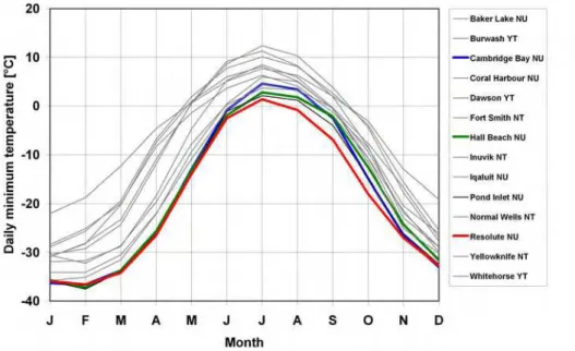
The cold climate protocol was developed using weather data extracted from one cold location. The selection of this representative location was made from a pool of locations for which long-term data sets of hourly weather conditions were available. Many of the locations had up to 48 years of data, starting as early as 1953, and ending in 2001. To winnow the list of potential locations, only locations that met the cold climate criteria outlined by Cornick (2005) were considered. The criteria were: 1) 100 or more days where daily min. is less than –20oC, and/or 2) 8000 or more heating degree-days below 18oC. Fig. 1 shows the mean min. daily temperatures for locations with long-term data meeting the criteria. The three coldest populated locations considered were Cambridge Bay (Iqaluktuuttiaq), Hall Beach (Sanirajak), and Resolute (Qausuittuq), all in Nunavut. Of the three possible locations with long-term data, Cambridge Bay was selected as the representative location. Cambridge Bay shows the greatest seasonal temperature range.
3.2 Temperature
Winter. Temperature was the most important testing parameter for the extreme protocol. Three seasons were considered; winter (Dec. to Feb.), spring (Mar. to May), and summer (Jun. to Aug.). In determining the thresholds for the winter season, min. daily temperatures were considered. The average min. temperature for the three winter months is –35oC, the suggested baseline for the winter temperature cycle. There are significant periods where the temperatures are –40ºC and below. A threshold temperature of –42ºC is proposed to mimic typical cold spells lasting about a week. There are significant periods when the temperatures drop below the winter design temperature, –46ºC (NBCC 2005). During these periods, the heating systems in buildings may not be able to maintain the design temperature. To simulate extreme cold spells, a threshold temperature of –50ºC held for 36-hours is proposed. The rates of temperature change in winter fall between 0 and 2ºC/h (Cornick 2008b). It was clear from the data that there is no regular pattern of diurnal temperature cycling during the winter season therefore no diurnal temperature cycling for the winter portion of the test protocol is provided. The suggested winter temperature profile for the cold regions protocol is given in Table 1.
Spring. There is a rapid warming during the spring season. Large diurnal cycles may result in melting and refreezing of moisture accumulated in the wall stud cavity. Daily max. temperatures are proposed as the basis of the spring season profile to increase the possibility of freeze/thaws in the cavity. Temperatures for the typical spring months vary significantly around the mean value. A steady warming trend was observed. Suggested steps are at –25ºC for March, –15ºC for April, and –5ºC for May. The rates of temperature change in spring fall between 0 and 4ºC/h, however most of the values fall between 0 and 2ºC/h. Data obtained for the spring months show a clear pattern of diurnal cycling due to insolation. To maximize the effect of springtime variation it is recommended that a 10ºC 24-hour diurnal swing around the base line temperatures be incorporated into spring season profile. The solar model assumes a simple symmetric cosine variation around the daily mean temperature shifted to accommodate the peak, at 16:00 hours (Cornick 2008b). The spring solar profile is given in Table 1.
FIG. 1: Mean daily minimum temperatures for various Northern locations.
Summer. The summer months show a progressive warming due to increased amounts of insolation. Regular diurnal cycles can raise the temperature of exterior envelope elements much above ambient temperature leading to possible heat damage or premature aging. To maximize the potential for such effects to occur in the test the daily max. temperatures were selected as the basis of the summer season profile. The mean max. temperatures for the typical summer months are 5oC, 15oC, and 10oC in steps. To simplify the protocol a single condition of temperature, 15C was selected. There was less variation in heating and cooling rates than in the spring. This is expected due to the prolonged daylight periods. Most of the rates of temperature change in summer fall between 0 and 2ºC/h although there were excursions of up to 8ºC/h. The summer months also show a strong pattern of diurnal cycling due to solar irradiance. The spring diurnal temperature profile is recommended (see Table 1).
3.3 Wind
Wind is an important climate parameter in the performance of exterior envelopes in extreme cold climates. The Canadian arctic can be divided roughly into two regions, the east and west, the Eastern Arctic being the windier of the two. Comparing various Northern communities, Cambridge Bay can again be used as a representative location for windy locations. The mean monthly mean wind speeds tend not to vary by season while the direction is consistent from the North. For the protocol a constant wind condition, 22 Km/h or 6.1 m/s, close to the annual mean, was suggested. To simulate wind in a test chamber a fan can be used or a pressure difference maintained across the sample to simulate the effect of wind. When using a pressure difference a heat transfer coefficient must be maintained on the exterior surface to simulate the effect of heat removal. In determining the appropriate pressure difference, ΔP, across the sample, the following assumptions were made: 1) the building height was 6m, 2) the location of the neutral pressure plane was at grade, 3) the station pressure was 101.3 kPa, 4) the indoor temperature was 25ºC, 5) the wind pressure coefficient on the leeward side was 1.0, and 6) the stack and wind pressures were added.
Wind velocity pressures at the wind speed recommended for the protocol vary from 23 to 30Pa, depending on temperature. The absolute stack pressure was calculated for various temperature differences. For the spring and summer time conditions the stack pressure is much reduced, approximately 5Pa. The wind velocity pressure and stack pressures were added to give the worst case. For the winter profile, assuming an ambient temperature of – 35ºC, the long-term mean, and the wind velocity pressure is approximately 27Pa. The stack pressure at this temperature is approximately 17Pa. The combined pressure is 44Pa. Rounding up the recommended pressure difference across the envelope was 50Pa. The recommended spring and summer period pressure differences across the envelope were 35Pa and 25Pa respectively. The variation of Heat Transfer Coefficient (HTC) using the ASHRAE Handbook of Fundamentals, Chapter 3 formula (ASHRAE 2005, McAdams 1954) shows that the heat transfer coefficient should be in the range of 30 W/m2·K for the wind speed recommended. The suggested pressure difference and heat transfer coefficient profile is given in Table 1.
TABLE 1: Parameters that comprise the exterior protocol, the complete protocol is given by Cornick (2008b).
Stage No. Season Description Ext. T [°C] Time [h] ΔP Pa/HTC [W/m2·K] RH [%]
1 Winter Initial conditioning –35ºC 168 50/30 70
2 Winter Average conditions –35ºC 168 50/30 70
3 Winter Typical conditions –42ºC 168 50/30 70
4 Winter Extreme conditions –50ºC 36 50/30 70
5 Winter Average conditions –35ºC 168 50/30 70
6 Spring Spring (Mar.) –25ºC 72 35/30 80
7 Spring Spring (Apr.) –15ºC 72 35/30 80
8 Spring Spring (May) –5ºC 72 35/30 80
9 Summer Summer season 15ºC 120 25/30 85
3.4 Atmospheric Moisture
Atmospheric moisture in the extreme cold regions does not directly play a large role in the performance of the envelope. Temperatures are too cold throughout most of the year for the atmosphere to hold significant amounts of moisture. The importance of this parameter depends largely on the interior environment. During the winter months the average humidity ratio is about 0.6 g water g/kg dry air. For the temperatures specified for the winter portion of the protocol the saturation humidity ratios are less than 0.14 g/kg. Compare these values with typical values for indoor moisture content, which vary between 2 and 4 g/kg during the winter. Control of humidity on the cold side of the test chamber is not crucial during the winter portion of the test protocol. If humidity control is desired and possible, a suggested target RH is 70% for the winter portion of the test. In spring, like the winter months, the amount of water vapour in the atmosphere is still low. The average humidity ratio is about 1.0 g/kg. If humidity control is desired and possible, it is suggested that the target RH be held at 80% for the spring part of the test. In the summer months the average humidity ratio is 5.0 g/kg. This is more significant than the other periods. The suggested target RH is 85% for the summer part of the test. The RH profile is given in Table 1.
3.5 Insolation
The decision to include solar radiation in the cold regions test protocol was based on anecdotal evidence provided by building specialists in Northwest Territories during community consultation, to the effect that solar driven moisture was a major consideration with respect to performance and premature aging of materials on
certain building facades (Cornick and Rousseau 2007). Global horizontal radiation in Cambridge Bay NU shows a sharp rise in the spring months and a sharp fall off in the autumn with a slight double peak. The direct irradiance pattern follows a similar pattern but shows a more pronounced double peak. Diffuse radiation reaches a peak on the longest day of the year. The pattern on a vertical surface is different. In Cambridge Bay the south orientation receives the most radiation. The peaks occur at the end of March or beginning of April. The peak solar radiation received on a southern exposure occurs during the spring swing season around Day 93 (April 3rd). The peak mean total irradiance corresponds with the peak mean hourly irradiance as well. Day 93 is suggested for the solar profile for the spring portion of the exterior test protocol. Direct solar irradiance on a vertical surface is less in the summer months than in spring. Diffuse radiation is high due to the longer daylight hours. The peak values occur towards the beginning of June. Since there is almost constant daylight for the summer months, the direct and diffuse profiles are all similar. The suggested daily profile occurs on the summer solstice (June 21st or Day 172). The hourly irradiance values, direct normal plus diffuse, rounded to the nearest 20 W/m2 for practical purposes are given in Table 2. The values given are direct normal radiation on a south facing vertical surface plus the diffuse radiation. The recommended irradiance for the winter is 0 W/m2.
Table 2: Mean total irradiance W/m2 for selected days on a south face vertical surface in Cambridge Bay NU.
Season/Hour Day 1 2 3 4 5 6 7 8 9 10 11 12 Spring 3 April 0 0 0 0 0 20 40 180 380 580 720 820 Summer 21 June 20 20 40 40 80 100 120 180 280 360 440 500 Season/Hour Day 13 14 15 16 17 18 19 20 21 22 23 24 Spring 3 April 860 820 700 540 360 160 20 0 0 0 0 0 Summer 21 June 520 520 460 360 260 160 100 80 60 40 20 20
4. Interior extreme cold climate test protocol
The interior test protocol for the cold regions was based on measurements undertaken in 16 homes in Inuvik Northwest Territories and Carmarks Yukon Territory (Rousseau et al. 2007, Cornick and Kumaran 2008).
4.1 Temperature
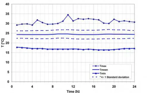
From the measurement data, the following observations were made, 1) temperatures were kept high, 2) the ranges are different; 5°C to over 35°C for Carmacks, 16°C to 35°C for Inuvik, 3) the mean temperatures in the Carmacks and Inuvik data sets were similar, and 4) there was considerably more variability in the Carmacks data. There were two distinct patterns in the data. The difference in the data sets was that the majority of the Yukon houses surveyed were heated using wood burning stoves without heat distribution systems. Since the majority of houses in the Arctic are not heated by wood, a heating profile was developed using the Inuvik data, i.e. houses with forced-air or baseboard heating systems. In houses with working heat distribution systems temperatures were kept high, temperature control was good, and the range was narrow (see Fig. 2). Setbacks were not used. Several Nordic residents where occupants tend to use high set points and open windows for temperature control confirmed this anecdotally. The recommended profile is 21ºC, the 10% temperature. In houses that use wood stoves, temperature control was more variable and setbacks were observed when the occupants were away or sleeping. Seven of the eight houses surveyed in the Yukon used wood burning stoves as the primary heat source. There were no central heat distribution systems or thermostats. A separate temperature profile was developed for houses with wood burning stoves, details of which are given by Cornick (2008a). Spring and summer temperatures for the cold locations were not measured as part of the project. Predictions of the interior temperatures were based on the procedure outlined in ASHRAE 160P (2006). Springtime temperatures for Cambridge Bay NU are still cold. Interior temperatures in the spring were set to 21°C. The month chosen for summer was July 1983 a typical warm summer month. The 24-hour running average temperature never rises above 18.3°C consequently the summer profile is set at a constant 21°C.
4.2 Relative humidity
Three strategies for setting the boundary relative humidity conditions on the room side were examined: 1) constant conditions, 2) an offset from the exterior conditions, and 3) an interior daily moisture profile.
FIG. 2: Hourly temperatures for the houses surveyed, Inuvik NT. Minimum, maximum and mean temperatures of the houses surveyed for each hour of the day, plus or minus one standard deviation are shown.
4.2.1 Constant conditions
The sample period for the surveys was in winter. The 90th percentile value of the combined dataset was chosen for the RH level threshold. The RH at this level was 41%, rounded down to 40%. This threshold is in line with the recommended value in ASHRAE 160P (2006). Spring and summer data for Inuvik and Carmacks were not measured as part of the project. Predictions of the interior RH were based on the procedure outlined in ASHRAE 160P. For the representative location the month chosen was May 1991. The mean daily temperature for May was –5.3°C, which using the procedure yielded a relative humidity of 44.7% rounded up to 50%. Similarly for summer RH conditions the month chosen was July 1983. The mean daily temperature for July was 12.3°C, which using the procedure yielded a relative humidity of 62.3%, rounded up to 65%.
4.2.2 Dynamic/Offset
Another method proposed was to use an offset from the exterior conditions, applied to the interior chamber of the test facility. The offset expressed in terms of difference between indoor and ambient humidity ratio was determined from the survey data in a manner similar to that used in determining the constant RH conditions. A lognormal distribution was assumed. In selecting the moisture load threshold for the test protocol the 90% value of the combined dataset was chosen. The moisture load at this level is 5.0 g/kg. It was suggested that this moisture loading, be used for all seasons, since there was no data to suggest that the loading was seasonal.
4.2.3 Interior moisture profile
A daily moisture profile based on the survey results was produced. The profile accounts for moisture added to the interior during the day. The advantages of this method are that a typical 24-hour profile can simulate typical occupant behaviour and other profiles exist for comparison. The disadvantage of the approach is that it may be difficult to achieve in the lab. Examples of daily moisture profiles already exist (Ellinger 2004). Tariku (2008) developed a moisture profile by estimating the daily moisture generation based on occupancy (Christian 1994), determining a schedule for the occupants, then distributing the moisture according to the schedule. In the case of the survey data it was difficult to generate a moisture generation schedule lacking information on occupancy, house characteristics, and the use of ventilation equipment. A moisture profile based on the measured data that imposes humidity conditions rather than imposing a load added to ambient conditions was developed. The humidity ratio was derived from the recommended RH and temperature profiles.
Different rooms type were monitored, bathrooms, kitchens, bedrooms, common areas, and storage spaces. Certain rooms have a specific use and distinct moisture profiles. A generalized profile is shown in Fig. 3. There was much data on bathrooms and kitchens. Three profiles were generated: 1) a bathroom profile, 2) a kitchen profile, and 3) a whole house profile. The normalized mean RH for each hour in each room was plotted in order
to identify patterns. The thresholds were based on statistical analysis. The hourly profiles are given in Table 3. Profiles for the other time steps were also developed (Cornick 2008a).
5. Discussion
Testing protocols developed for the assessment of the hygrothermal performance of building envelope for extremely cold regions, such as the Arctic are scarce. The protocols here may be furthered refined as actual testing experience is acquired. The key to developing the exterior protocol was the selection of a representative location. Other locations may be selected, however, the methodology for determining the thresholds values remains valid (Cornick 2008b). No account was made for increasing temperatures in the Arctic. Recently the Canadian meteorological service has made the modelling data on the Intergovernmental Panel on Climate Change 4th Assessment Report (IPCC 2007) scenarios available. A reassessment of the exterior protocol is perhaps in order to reflect future trends. With respect to the interior protocol more survey data is required, particularly for spring and summer seasons. Although there was sufficient data for developing the winter portion of the interior protocol, the survey pointed to areas where more information would be useful. Specifically, more information on specific rooms, a better assessment of air-change rates, air pressure difference and occupant behaviour are required. As well, a longer monitoring program needs to be established to provide hourly data on the interior conditions throughout all seasons.
Fig. 3: A generalized moisture profile. TABLE 3: Hourly whole house profile
Time [h] RH [%] T [°C] W [g/kg] Notes Time [h] RH [%] T [°C]W [g/kg] Notes
Whole house average
0 10 21 1.5 10thpercentile 16 40 21 6 90th percentile 7 40 21 6 90thpercentile 20 20 21 3 Mean 8 20 21 3 Mean 23 10 21 1.5 Mean Bathroom Profile 0 10 21 1.5 10th percentile 18 50 21 8 99th percentile 7 50 21 8 99th percentile 20 20 21 3 Mean 8 20 21 3 Mean 23 10 21 1.5 Mean Kitchen Profile 0 10 21 1.5 10th percentile 16 40 21 6 90th percentile 7 40 21 6 90th percentile 20 20 21 3 Mean 8 20 21 3 Mean 23 20 21 3 Mean
6. Summary
This paper gives an overview of the development of two test protocols for testing building envelopes exposed to extreme cold conditions as found in the Canadian Arctic. The exterior protocol comprises four parameters:
temperature, wind, atmospheric moisture and solar irradiance. An accelerated test was defined; the length of the test is 6 weeks or 42 days. Three seasons comprise the test, a winter season, a spring or swing season and a summer season. Not all the parameters need to be used in the test. The most important parameter is temperature. Other parameters can be added as required. A corresponding interior test protocol was also developed. The protocol comprises two parameters: temperature and moisture. The protocol was based on the results of monitoring the indoor environment of 16 residential units for one winter month.
7. References
ASHRAE. (2005). Fundamentals, Atlanta, Ga.: Am Soc of Heating, Refrigerating and Air-Conditioning Eng. ASHRAE. (2006). SPC 160P, Public Review Draft Sept 2006. Atlanta, Ga.
Christian J. E. (1994) Moisture Sources, “Moisture control in buildings” Heinz R. Trechsel, ed. ASTM, Philadelphia, Pa. Chapter 8.
Cornick, S. M., M. Manning, M. Z. Rousseau, M. C. and Swinton. (2008a). Task 5 Proposed Test Protocol for Walls of Houses in Extreme Cold Regions Part 2: Defining Interior Conditions, NRC-IRC Client Report B1239.6 2008.
Cornick S. M. (2008b). Task 5 Proposed Test Protocol for Walls of Houses in Extreme Cold Regions Part 1: Defining Exterior Conditions, NRC-IRC Client Report B1239.5 March 2008.
http://irc.nrc-cnrc.gc.ca/pubs/fulltext/b-1239.5/
Cornick S. M. and Kumaran M. K. (2008). A Comparison of Empirical Indoor Relative Humidity Models with Measured Data, Journal of Building Physics Vol. 32. No. 1. pp. 243-268.
Cornick, S.M.; Rousseau, M.Z. (2007). Community Consultation on Wall Construction Methods, Institute for Research in Construction, National Research Council Canada, IRC-RR-233 pp. 25 June 2007. http://irc.nrc-cnrc.gc.ca/pubs/rr/rr233/
Cornick, S.M. (2005). Task 3: Report on Task 3: Extreme Canadian Climates - Northern and Coastal, pp. 60, July, 2005 http://irc.nrc-cnrc.gc.ca/pubs/fulltext/b-1239.3
Ellinger, M. (2004). Feuchtepufferwirkung von Holzinnenraumverkleidungen. University of applied science Rosenheim. Thesis.
IPCC (2007). Climate Change 2007: Fourth Assessment Report, http://www.ipcc-data.org/ddc_ar4pubs.html Kovesi T, Creery D, Gilbert N.L., et al. (2006a). Indoor air quality risk factors for severe lower respiratory tract
infections in Inuit infants in Baffin Region, Nunavut: a pilot study. Indoor Air 2006; 16:266-75.
Kovesi T, Stocco C, Dales R,E,, et al. (2006b). A multi-community survey of indoor air quality risk factors for severe lower respiratory tract infections (LRTI) in Inuit infants in Baffin region, Nunavut, Canada [abstract]. Proc Am Thorac Soc 2006;3:A397.
Maref, W, Manning, M.M., Lacasse, M.A. et al. (2007) "Laboratory demonstration of solar driven inward vapour diffusion in a wall assembly," 11th Canadian Building Science and Technology Conference Banff, Alberta, March 22, 2007, pp. 1-8, (NRCC-49203) http://irc.nrc-cnrc.gc.ca/pubs/fulltext/nrcc49203/
Masters, L. W. and W. C. Wolfe. (1974). The Use of Weather and Climatological Data in Evaluating the Durability of Building Components and Materials, NBS Technical Note 838, Institute for Applied Technology, National Bureau of Standards, Washington D.C. 20234.
McAdams, W. H. (1954). Heat Transmission, 3rd edition, McGraw Hill, New York
Mehlhorn L. and J. W. Herlyn. (1998). Bauteilentwicklung durch simulierte Bauteilprüfung in der
Doppeklimakammer, Bauen mit Holz und Holzwerkstoffen: Stand der Technik und Entwicklungstendenzen Braunschweig (Deutschland, Bundesrepublik):Selbstverlag 1998, S.1-14, Abb.,Lit. Serie: WKI-Bericht; 33, (Development of Building Components through simulated testing of Building Components in a ‘Double Climate Chamber’ TT).
NBCC (2005). National Building Code of Canada, Canadian Commission on Building and Fire Codes, National Research Council of Canada, Ottawa, Volume 1: Division B, Appendix C, Table 9.25.1.2, p. 9-141
Rousseau, M., M. Manning, M.N. Said, et al. (2007). “Characterization of Indoor Hygrothermal Conditions in Houses in Different Northern Climates”, Thermal Performance of the Exterior Envelopes of Whole Buildings X International Conference, Clearwater Beach, FL, pp. 14, Dec. 2-7.
Saïd, M. N. (2005). Building envelope researchers to develop wall assemblies suited to construction north of 60°. Construction Innovation. Institute for Research in Construction National Research Council Canada. 10: 9. Saïd, M. N. (2006). Task 2: Literature Review: Building Envelope, Heating, and Ventilating Practices and
Technologies for Extreme Climates, pp. 120. http://irc.nrc-cnrc.gc.ca/pubs/fulltext/b-1239.2/
Tariku F. (2008). Whole Building Heat, Air, and Moisture Analysis, PhD Thesis, Concordia University, April 2008.