Analysis and design of developable surfaces for shipbuilding

(1)

Analysis and Design of Developable Surfaces for Shipbuilding

by

Julie Steele Chalfant

B.S., Mechanical Engineering

United States Naval Academy, 1988

Submitted to the Department of Ocean Engineering

and the Department of Mechanical Engineering

in partial fulfillment of the requirements for the degrees of

Master of Science in Naval Architecture and Marine Engineering

and

Master of Science in Mechanical Engineering

at the

MASSACHUSETTS INSTITUTE OF TECHNOLOGY

June 1997

@

Massachusetts Institute of Technology 1997. All rights reserved.

A uthor.

.. .

...

..

• ... ...

Department of Ocean Engineering

May 9, 1997

Certified by

...

Nicholas M. Patrikalakis

Professor of Ocean Engineering

Thesis Co-Supervisor

Certified by

. ...

...

Takashi Maekawa

L,ort~rer and Research Scientist

/

Thesis Co-Supervisor

C ertified by

...

.

...

... - ...

David C. Gossard

Professpr of Mechanical Engineering

rhesis Reader

Accepted by.

...

J. Kim

Vandiver

Chairman. DTa-atmental Committee on Graduate Students

DeDartment of Ocean Engineering

A

ccepted by ...

.. ...

Ain

Sonin

Chairman, Departmental Committee on Graduate Students

Department of Mechanical Engineering

JUL 1

5 1997

a"n

(2)

(3)

Analysis and Design of Developable Surfaces for Shipbuilding

by

Julie Steele Chalfant

Submitted to the Department of Ocean Engineering and the Department of Mechanical Engineering

on May 9, 1997, in partial fulfillment of the requirements for the degrees of

Master of Science in Naval Architecture and Marine Engineering and

Master of Science in Mechanical Engineering

Abstract

A developable surface can be formed by bending or rolling a planar surface without

stretch-ing or tearstretch-ing; in other words, it can be developed or unrolled isometrically onto a plane. Developable surfaces are widely used in manufacturing with materials that are not amenable to stretching. A ship hull design entirely composed of developable surfaces would greatly reduce production costs of that hull.

This thesis describes a new, user-friendly method of designing developable surfaces with a B-spline representation. First, it expands the work of Aumann in designing developable B-spline strip surfaces whose directrices lie on parallel planes. The computer program developed can assist in designing surfaces from curves of any degree with any number of segments, and includes a test for regularity. Second, a new method is developed which permits the design of developable surfaces with general three-dimensional space curves as directrices. The computer program permits design of degree (3-1) B-spline developable surfaces with two patches using a minimization process. The basis is provided to extend this to surfaces with more patches and higher degrees. A test is provided to ensure that the minimization process results in a developable or nearly developable surface. This method is extended to include special interesting cases such as triangular degenerate patches and surfaces with a planar resulting directrix.

This thesis also treats common differential geometry properties such as lines of curvature and geodesics that are useful in the design and manufacturing process. Lines of curvature are vital in the forming process, since the planar shape must be placed so the rollers are parallel to the lines of zero curvature. As an inflection line greatly affects the forming process, a method is described to determine the inflection line in advance; several properties of developable surfaces related to inflection lines are also described.

Straight lines on a plane map to geodesics on a developable surface. This fact is of assistance in many aspects of the use of developable surfaces, including layout and quality control. A method is described to calculate geodesics on a developable surface as an initial value problem instead of the more complicated boundary value problem.

Engineering examples are provided for each topic, and a small boat hull is designed using the methods described. In addition, recommendations for further research are made. Thesis Co-Supervisor: Nicholas M. Patrikalakis, Professor of Ocean Engineering

Thesis Co-Supervisor: Takashi Maekawa, Lecturer and Research Scientist Thesis Reader: David C. Gossard, Professor of Mechanical Engineering

(4)

Acknowledgements

I would like to express my sincere appreciation for the guidance provided by Dr. Takashi Maekawa and Prof. N. M. Patrikalakis. I would additionally like to thank Prof. D. C. Gos-sard for his assistance, Mr. Stephen Abrams and Mr. Fred Baker for their assistance with computer work, Dr. Xiuzi Ye for his feedback, and the members of the Design Laboratory including Dr. Wonjoon Cho, Mr. Todd Jackson, Mr. Guoling Shen and Mr. Guoxin Yu for their support.

Special thanks to LT Allan Andrew, LT Kurt Crake, LT Tom Laverghetta, LT Chris Levesque, LT Casey Moton, and LT Tom Trapp for their camaraderie and support, and to LCDR Mark Welsh and CAPT Alan Brown.

(5)

List of Figures

2-1 Tangent Vector ... ... 14

2-2 Osculating Plane ... 15

2-3 Space Curve ... 17

2-4 Curvature Vectors ... 20

3-1 A Cubic Bezier Curve with Control Polygon . ... 26

3-2 The deCasteljau Algorithm ... 27

3-3 A Bezier Surface with Control Net ... 28

3-4 Continuity Conditions ... 29

3-5 A Cubic B-spline Curve Segment with Control Polygon . ... 30

3-6 Convex Hull Property for a Cubic B-Spline Curve . ... 31

3-7 The deBoor Algorithm ... . . . ... ... . . . . . 32

3-8 Knot Removal . ... . .. . . . . ... . . ... . . 34

4-1 A Ruled Surface ... 38

4-2 A Developable Surface with Tangent Plane along a Ruling . ... 38

4-3 An Envelope of a Family of Curves ... 40

4-4 Edge of Regression ... 41

4-5 A Surface with Folds and a Developable Surface . ... 44

5-1 A Developable Surface ... 48

5-2 Design of Developable B-Spline Strip Surface . ... 50

5-3 Effect of Simple Bounds on Developable Surfaces . ... 57

5-4 Design of Developable B-Spline Surfaces . ... . 61

5-5 Planar Constraint on Developable B-Spline Surface Design ... 64

5-6 Triangular Degenerate Cubic B6zier Patch . ... 66

5-7 Development of B-Spline Developable Surface . ... 69

5-8 Automobile Windshield, a Developable Degree (4-1) B-spline Strip Surface 70 5-9 Ship Stack, A Developable Degree (3,1) B-Spline Surface with

IKI

< 2.19 x 10- 7 . . . . .. . . .. .. 71

6-1 Geodesics on a Closed Surface ... 74

6-2 Geodesic on a Degree (3,1) Developable Surface . ... 75

6-3 Geodesic on a Degree (4,1) Developable Surface . ... 78

6-4 Geodesic on a Degree (4,1) Handkerchief-like Developable Surface ... 79

7-1 Developable surface and its control polyhedron with inflection line. ... 86

7-2 (a) Lines of curvature of developable surface with inflection. (b) Magnifica-tion near inflecMagnifica-tion line. ... 86

(8)

7-3 (a) Lines of curvature on perturbed surface ( = 0.02. (b) Magnification near

u=0.57 ... . . .. ... 87

7-4 (a) Lines of curvature on perturbed surface ( = 0.08 (b) Magnification near u=0.57. ... 87

8-1 Planing Boat Terminology ... 89

8-2 Boat Composed of Developable Degree (3-1) B-Spline Surfaces ... . 91

8-3 Boat Bottom View ... 91

8-4 Boat Surfaces Developed onto a Plane ... .. 92

8-5 Geodesics on the Forward Side Section ... .. 93

8-6 Lines of Curvature on Boat Surfaces (Solid Lines are Maximum Curvature Lines, Dashed Lines are Minimum Curvature Lines) ... 94

(9)

List of Tables

6.1 Control Points for a Degree (3,1) Developable Surface . ... 77

6.3 Control Points for a Degree (4,1) Handkerchief-like Developable Surface . . 79

8.1 Target Curve Data ... 90

(10)

(11)

Chapter 1 Introduction

1.1 Background and Motivation

A ruled surface is a curved surface which can be generated by the continuous motion of a straight line in space along a space curve called a directrix. This straight line is called a generator, or ruling, of the surface. Developable surfaces are a subset of ruled surfaces which have the same tangent plane at all points along the generator. A developable surface can be formed by bending or rolling a planar surface without stretching or tearing; in other words, it can be developed or unrolled isometrically onto a plane. Developable surfaces are also known as singly curved surfaces, since one of their principal curvatures is zero.

Developable surfaces are widely used in manufacturing with materials that are not amenable to stretching. Applications include the formation of ship hulls, ducts, shoes, clothing and automobile parts such as upholstery and body panels [14].

In shipbuilding, developable surfaces are shaped using only rollers or presses. Heat treatment is then used only to remove distortion induced by welding or other means. Dou-bly curved surfaces, on the other hand, must be heat treated after rolling to induce the additional curvature. The heat treatment is normally done by hand, by a skilled artisan with years of training to achieve the correct amount of bending. This is an extremely time consuming, labor intensive and thus expensive process.

According to Avondale/IHI Shipbuilding Technology Transfer data for a tanker, only 15.1% of the curved plates in a ship hull are singly curved, while 65.8% of the plates are doubly curved, requiring roller and heat treatment processes [28]. An intensive effort to increase the amount of developable surfaces in the hulls of merchant ships at Burmeister & Wain Shipyard [34] has resulted in a reported 20% reduction in manhours required to produce a hull. Designing a ship entirely of singly curved, or developable, surfaces would reduce construction costs even more.

Recently researchers in Computer Aided Geometric Design have been quite active in investigating the representation of developable surfaces in terms of Non-Uniform Rational B-Spline (NURBS) surfaces or a special case of NURBS called B6zier surfaces [1, 3, 14, 29]. NURBS curves and surface patches are the most popular representation method in CAD/CAM due to their generality, excellent properties and incorporation in international standards such as IGES (Initial Graphics Exchange Specification) and STEP (Standard for the Exchange of Product Model Data). Thus, it would be beneficial to design developable surfaces using a B-spline representation.

(12)

1.2 Research Objective

Recently, efforts have been underway to revitalize commercial shipbuilding in the United States. Several professors at MIT are involved with developing cost saving methods in ship fabrication to ensure that shipbuilding in the US will be competitive in the world market. This research is in support of one of those efforts.

The main goal of this research is to develop a user-friendly method of designing devel-opable surfaces with a B-spline representation. The effort is then extended to address some common differential geometry properties that will be useful in the design and manufacturing process.

The ultimate goal is to provide a method to design a complete ship hull from developable surfaces and to generate cutting and bending information in a format that is user friendly for both the engineer and the worker. Although this thesis does not go that far, it takes a major step toward this goal.

1.3 Thesis Organization

In this thesis, Chapters 2 through 4 review basic differential geometry properties and intro-duce the concepts of developable surfaces. They also briefly review the Bezier and B-spline representations of curves and surfaces. The information introduced in these chapters will be used throughout the thesis.

Chapter 5 describes a new user friendly method for design of developable surfaces in B-spline representation. Section 5.1 reviews the current literature on developable surfaces. Section 5.2 describes the design of strip surfaces that are constrained between two parallel planes. Section 5.3 describes the design of surfaces with directrices that are space curves and treats special cases such as triangular degenerate patches and surfaces with a planar resultant curve. Section 5.4 describes the unrolling, or development, of the surfaces into a plane. Section 5.5 gives some engineering examples.

In Chapter 6, a geodesic on a developable surface is found as the solution to an initial value problem rather than a two point boundary value problem. The geodesics can be used in ship design for laying out butts and strakes, among other uses. In Chapter 7, the lines of curvature on a developable surface are analyzed and the line of inflection is defined. These concepts are required for the bending of steel plates into developable surfaces; the steel must enter the rolls in a direction parallel to the lines of zero curvature, and cannot be rolled past a line of inflection [33].

A small boat was designed using the methods described in this thesis. The boat is presented in Chapter 8 as a practical engineering example.

The thesis concludes with Chapter 9 which includes recommendations for further re-search.

(13)

Chapter 2 Review of Curves and Surfaces

2.1 Introduction

This chapter reviews the basic theory of curves and surfaces including such topics as the Serret-Frenet formulae, the first and second fundamental forms, curvatures and geodesic curves which will be used in derivations of many formulae in the later chapters. The information in this section follows the derivations in classical texts on differential geometry and geometric modeling such as those by Kreyszig [26], Struik [41] and Faux and Pratt [11].

2.2 Basic Theory of Curves

Throughout this thesis, curves are represented in a parametric manner, r(u), as a function

of one parameter, u, that lies within a closed interval ul < u < u2. The curve is a mapping

from a one parameter interval to three-dimensional space

r(u) =

[x(u)

y(u) z(u)]T.

The points on a curve are regular as long as at least one of the first derivatives is not equal

to zero. In other words, a point is singular if dx/du = dy/du = dz/du = 0. The curve can

be reparameterized if u can be expressed as u = f(ul) as long as du/dul

#

0.

Arc length is defined as the distance along a curve between parameter values u0 and u,

and can be represented as

s (u)= .2+ 2 j2 du =j 7 du. (2.1)

In this thesis, derivatives with respect to the arec length s will be represented by a prime and derivatives with respect to u will be represented by a dot. Derivatives of arc length s with respect to parameter u and vice versa are

= ds -du =. d Vi7 r-4 du = du 1

ds

i-l

(14)

duf du'

ds ( . .)2'

The unit tangent vector t to a curve is defined by the unit vector that passes through two points in the curve, r(s) and r(s + h) (see Figure 2-1), as h approaches zero; i.e.

r(s + h) - r(s) dr

t = lim = r'(s)

h-O0 h ds

dr(u) du _ (u)

du ds

i-(u) I

This final representation clearly shows that t is a unit point r(un) in the direction of t(un) is the tangent to

vector. The line passing through the the curve at un.

Figure 2-1: Tangent Vector

All vectors normal to t(un) at Un lie in a plane called the normal plane. Much as the tangent is defined by two points that approach one another on a curve, the osculating

plane is defined by three points that approach one another. In other words, the osculating

plane is the plane in which the curve lies at a point on the curve. If the curve is planar, the entire curve lies in a single osculating plane, and the osculating plane is constant for the entire curve. To mathematically define the osculating plane following the derivation in

Kreyszig [26, p.31], take three points at parameter values u, u + hi and u + h2. The plane

can be defined by the two linearly independent vectors ai = r(u + hi) - r(u), i = 1, 2 or

linear combinations thereof. Let

(i) r(u + hi) - r(u)

hi

and

2(v(2) - V(1))

w h=

(15)

The Taylor series expansion of r(u + hi) is

r(u + hi) = r(u) + hir(u) + r ix(u) + o(h?)

where o(hn) is a vector of Landau symbols o(hn_{) with the property that [41, p.3]}

lim = 0.

h-O hn

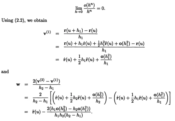
Using (2.2), we obtain

r(u + hi) - r(u) hi

r(u) + hlir(u) + ½h 2i(u) + o(h 2) _{- r(u)}

1 .

o(hl)

=

i(u)

+ -hl(u) +hi

2 hi and

2(v(

2

)

(1))

h2 - hi

2 - hi(u) + h2 (u) + h2 2(hio(h2) - h2

o(h2))

hih

2(h2 - hi) - ((u) + hli(u) +

As hi -+ 0, v( 1) -+ i(u) and w --+ i(u). Therefore, the osculating plane is defined by i-(u)

and i(u). Note that r(u) must be at least twice continuously differentiable.

plane

Figure 2-2: Osculating Plane

The principal normal is defined as the intersection of the osculating and normal planes.

Using an arc length parameterization, we find that differentiating t - t = 1 with respect to

(16)

s yields

t - t' = 0,

so t' is perpendicular to t and lies in the normal plane. Since t = r' = iu',

t' = ruI" + i(u')2

Thus t' lies in the plane of r and i, and therefore in the osculating plane. Since t' lies in

both the osculating and normal planes, a unit vector in the direction of t' is the unit normal

vector

t'

The magnitude of t' is called the curvature and is represented as n. The curvature vector k is represented as

k = t' = nn. (2.3)

A physical sense of the curvature can be found from the simple example of a line, which

has a constant tangent vector, so t' is zero. Therefore, ic = It'l = 0, and a line has zero

curvature. Parameterized by u, k and n can be represented as [41, p.16] k = t' = iu" +i(u') 2 = ( - (' 2 (j. j)2

•2

=

) (Kn

)

=[

i

[

(i' x

i)

(

x r)

I (j- . j-)2 1 (j. j)(2 (.j.)3

where the Lagrange identity (a x b) - (a x b) = (a - a)(b - b) - (a - b)2 is used.

The normal to the osculating plane is the binormal, which is defined as

b = tx n.

Since these three vectors are unit vectors that are mutually orthogonal, they satisfy the relations

b-b=1 n-n=1 t.t=1

b n=0 n-t=O t-b=0.

Differentiating b b = 1 and b - t = 0 yields

b'b = 0 and

b' - t = -b - t' = -b- K-n = -n(b. n) = 0.

Therefore, b' is orthogonal to both b and t and must then be parallel to n. Let

(17)

where r is the torsion of the curve. A physical sense of torsion can be found from the fact that a curve with zero torsion and nonzero curvature is a planar curve.

Finally, an equation for the derivative of the normal vector corresponding to the rate of

change of the tangent plane [26, p.41] can be determined. Differentiating n - n = 1 yields

n - n' = 0. Therefore, n' is orthogonal to n and must satisfy the relationship

n' = at + pb. (2.4)

Multiplying equation (2.4) by t and b respectively yields a=n' . t and /3=n'-b.

Differentiating n - t = 0 yields

a = n' - t = -n -t' = -n - nn = -r.

Similarly, differentiating n - b = 0 yields

p8

= n'. b = -n b' = -n - (-Tn) = 7. Thus,

n' = -rt + rb.

The representations of the derivatives of the three defining vectors for a curve are termed the Serret-Frenet formulae [41, p.18]

t' = n

b' = -rn

nw = -at + ,b,

which describe all aspects of a space curve, as shown in Figure 2-3.

I

Osculating Plane Norma

- -Tangent Plane

(18)

2.3 Basic Theory of Surfaces

A general parametric surface can be defined as a vector-valued mapping from a

two-dimensional parametric uv-space to three-two-dimensional space

R(u,v)

=

[z(u,v) y(u,v) z(u,v)]T,

where the two parameters u and v lie in the closed intervals ul < u < u2 and vi

<

v < v2.

The surface is regular at all points where the matrix

M = Ou Ou OU (2.5)

Ov Ov Ov

has rank 2, or equivalently Ru x Rv 0 [41, p.56]. Partial derivatives of a surface will be

represented as

OR OR

Ru = and Rv = .

du

Ov

A curve on the surface is represented as r(u, v) with u = u(t) and v = v(t) or equivalently R(u(t),v(t)) = r(t). This occurs when the rank of the matrix (2.5) is 1 at every point.

When we keep u constant in R(u, v) by setting u = un, we have an equation for a curve

that depends only on v, and is thus called an isoparameter curve. Similarly, v = v, is also

an isoparameter curve. The vector

dR du dv

R +R, -(2.6)

dt dt dt

is tangent to the curve when u and v are functions of t. This is of course also a tangent to the surface. The tangent plane to the surface at any point is determined by the two vectors

Ru and R,. The normal to the surface is orthogonal to this plane. A unit vector in the

direction of the surface normal is given by

N = x (2.7)

IRu

x

Rv

Note that this definition of the normal vector is undefined when R, x R, = 0, supporting

the assertion that a point on the surface is singular if RU x R, = 0. This may be due to

the shape of the surface or the choice of parameterization. In Section 5.3.5, an alternative definition of N is explored for degenerate points.

Using the definition of arc length (2.1), the distance between two points on a curve on the surface is found by integrating

ds = -vdxdx + dydy + dzdz =

VNdR

• _dR. _(2.8)

Combining (2.6) and (2.8) yields the first fundamental form of the surface

(19)

where Note that E = Ru Ru, F=R- R I, G=R,·,. EG-F 2 2

= (R,

x

R,)

-(R

x

R)

)

2

=

(RU

x

R)

2

.

(2.9)

Thus, EG - F2 is always positive if the surface is regular.

The first fundamental form enables us to determine arc lengths, angles and areas on the surface. In order to determine curvatures, the second fundamental form is required. First, the curvature vector of the curve on the surface, found from equation (2.3), is split into its normal and tangential components

dt

k = d- kn + kg = KnN + kg

where kn is the normal curvature vector and an is the normal curvature of the curve on

the surface at that point. The tangential portion of the curvature vector, kg, is called the

geodesic curvature vector. It will be discussed in more detail later.

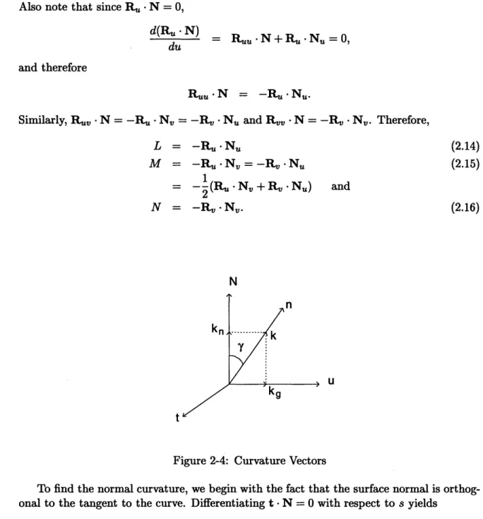
If the angle between the surface normal and the normal to the curve is designated 7 as

shown in Figure 2-4, then [26, p.118]

n

_-N

_{= cos((7)lnllNI =}

_cos(7)

from the definition of a dot product. Since t' = R" = n - n,

ncos()

=

-n -N

= R" N

= (Rudu + Rldv)'. N

= (Ru~dudu + 2Ruvdudv + RIvdvdv + Rud2u + Rvd2v) - N.

(2.10)

Since Ru N = R,

represented by

-

N = _{0, equation (2.10) reduces to the second fundamental form,}

II = (Ruududu + 2Ruvdudv + Rvdvdv) - N = Ldudu + 2Mdudv + Ndvdv where L = IR, N M = Ruv N N = RIv -N. and

(2.11)

(2.12) (2.13)

(20)

Also note that since R. - N = 0, d(R -

.N)

=R N

R, -N + R,. N, = 0,

du

and therefore

RI,

-N = -R. Nu.

Similarly,

R.,

- N = -R, - N, = -R, - Nu and R•,, N = -R, - N,. Therefore,

L = -R, -N M = -Ru-N, = -R.N 1 - (R, - N, + R, - N,) 2 N = -R N,. (2.14) (2.15) (2.16) and

Figure 2-4: Curvature Vectors

To find the normal curvature, we begin with the fact that the surface normal is

orthog-onal to the tangent to the curve. Differentiating t - N = 0 with respect to s yields

dt

dN

- N + t - = 0.

ds

Thus we have

dt

kN= s ds dN dR dN

dN

= -td

d

ds ds ds " Therefore,

dR dN =

(Rldu-Ln = -k MN= d" ds ds Ldudu + 2Mdudv + Ndvdv

- Rdv) - (Nudu + Ndv)

ds

2

Edudu + 2Fdudv + Gdvdv

II

(21)

--L + 2MX + NX2

S-L+2MA+NA 2 _(2.17)

E + 2FA

+ GA

2

where A = dv/du. The negative sign in equation (2.17) ensures that if rn is positive, the

center of curvature lies opposite to the direction of the surface normal.

Any point on the surface has many curves passing through it, each of which has an associated ~n. The maximum and minimum values of rn at a point are called the principal

curvatures of the surface at that point and are designated ,'i and K2. The maximum and

minimum values of Kn occur when dn = 0, [11, p. 112]

= (E + 2FA + GA2)(2M + 2NA) - (L + 2MA + NA2)(2F + 2GA) = 0. (2.18)

dX Using (2.18) in (2.17) yields L + MA M + NA E E+FA F + GA given

(E + 2FA + GA2₎ _{= (E}_{+ FA) +}_A(F_{+ GA) and}

(L + 2MA + NA2) = (L + MA) + A(M + NA).

Therefore the extreme values of an satisfy the two simultaneous equations

(L + anE)du + (M + anF)dv = 0 and (2.19)

(M + KnF)du + (N + KnG)dv = 0. (2.20)

These equations can be simultaneously satisfied if and only if

L+anE M+aKnF M+anF N+anG

The discriminant of this quadratic equation in Ian is greater than or equal to zero. Therefore

the equation has either two distinct roots cmax and smin, the maximum and minimum principal curvatures, or double roots rn, the normal curvature at an umbilical point. The corresponding directions A define directions in the uv-plane. The corresponding directions in the tangent plane are called principal directions of curvature and are always orthogonal except at umbilical points, where rImax and rmin are identical. In the special case where the identical principal curvatures vanish, the surface becomes locally flat. The two roots are given by

Kmax = H + V/H 2

- K and (2.21)

Kmin = H -

/H

2 _{-- K} _(2.22)

where K is the Gaussian curvature and H is the mean curvature defined by

LN - M 2

K = EG-F 2 (2.23)

EG - F2

2FM - EN - GL 2(EG - F2)

(22)

Using (2.21) and (2.22) in (2.23) and (2.24), it can easily be shown that

K = imax min H = (,max + min).

Note that at an umbilical point, H2 = K and at a flat point, K = H = 0.

The normal curvature can be represented in terms of the principal curvatures ni and K2

as

n = "K1 cOS2

(a)

+ 2 sin2 (a) (2.25)

where a is the angle between the direction dv/du and the direction dv = 0. This is known

as Euler's theorem [26].

Recall that the curvature vector of a curve on the surface can be split into its normal and tangential components

k = kn + kg,

where the tangential component, kg, is known as the geodesic curvature vector. Let u be a unit vector in the tangent plane perpendicular to t such that t, u and N form a

right-handed coordinate system in that order as shown in Figure 2-4. The geodesic curvature ag

can then be found from

kg = gU.

Additionally, since the magnitude of an can be represented as

Incos- l,

the magnitude of

ag can be represented as | sin 7y.

Geodesic curvature can be represented using only the first fundamental form. Since u. N = 0 and u u = 1,

dt

Kg = u k = u - d = u -t' = (Nx t) -t' = (tt'N). (2.26)

The unit tangent vector of the curve on the surface is given by

t = Ruu' + R v';

thus

t' = Ruu(U')2 + 2Ruvu'v' + Rv,(v')2 + Ruu" + Rvv". Therefore equation (2.26) can be rewritten as

Ki = (txt').N

= [(Ruu' + Rvv') x (Ruu(U')2 + 2Ruvu'v' + Rv,(v')2 + Ruu" + R,v")] " N

[(Ru x Ruu)(U')3 + (2Ru x Ruv + Rv x Ruu)(U')2v'

+(Ru x Rvv + 2Rv x Ruv)u'(v')2

(23)

Each of the coefficients of the combinations of u and v derivatives in (2.27) can be written in terms of the coefficients of the first fundamental form and their derivatives. For example,

(Ru x Ruu) - N

(R x Ruu)

-

(R, x R,)

VEG-

F2

(R, -R) (Ruu -Rv)

-

(R, -Ru) (R. -R,)

vEG- F2

2(E(Ruu Rv) - (Ru Ruu)F) EG - F2 2(EG- F2₎

(2EFu - EE, - FEu,)EG- F2

2(EG - F2₎

= F21 /EG-F 2

where 211 is one of the

form E, F and G and

Christoffel symbols defined by their derivatives, E,, F,, G,,

the coefficients of the first

E,, F, and G, fundamental GE, - 2FF, + FEv 2(EG - F2) GE, - FGu 2(EG - F2)' 2GF, - GG, + FGv 2(EG - F2)

2 _{_} _2EFU_- _{EE, + FE,}

11 - _{2(EG - F}2 )

r2 EG, - FE,

12 -

2(EG

_{- F}2₎

2 _{_} _EG,_- _{2FF, + FG,}

22 _2(EG_- _F2₎

Similarly reducing all the other coefficients in (2.27) yields

Kg

= [r2

(u')

3

+

(2rr

2

-

rl)(u')

2

v'

+

(r

2

-

2r

2

)U'(v')

2

-

rl(')

3

+u'v" - u" v'] /EG - F2.

(2.28)

A geodesic is defined as a curve with zero geodesic curvature [41]. Straight lines on a

surface are geodesics since the curvature vector k vanishes. For geodesics that are curved, the curvature vector coincides with the surface normal vector and, since the curvature vector lies in the osculating plane, the osculating and tangent planes are normal. The equation for

the geodesic can be obtained by setting ia9 equal to zero in equation (2.28), which yields

"v'-u'v"

=

Fl (u')

3

+ (212

Pl)(U')

1- 2

v'

+ (Fr

2

-

2F

2

)u'(v')

2 -_

12(U')

3

assuming that the geodesic is everywhere regular so EG - F2 is always positive. An

al-ternative representation for a geodesic is given by the set of coupled second order ordinary differential equations [41] duI 2

+

1 (d)2

F21 (ds

' _ds

S2r1

du dv

(dv)

2

+

22-2

_{ds ds}

22 _ds

= 0

2 du dv 2 dv2

+

2F2

_{ds ds}

± + 22 -&

_ds

= 0

where the two equations are related by the condition ds2 = Edu2+ 2Fdudv + Gdv2.

r11 d2u ds2 d2v ds2

(2.29)

(2.30)

(24)

(25)

Chapter 3 Curve and Surface Representation

3.1 Introduction

This chapter reviews the representation of curves and surfaces in Bezier and B-spline forms and treats the special properties associated with each. In addition, algorithms for knot insertion and removal, curve evaluation and splitting are summarized. The descriptions are based on texts by Hoschek and Lasser [22], Piegl and Tiller [36] and Yamaguchi [44].

3.2 Bezier Curves and Surfaces

Bernstein Polynomials

The Bernstein polynomials are defined as

Bi,n (u) = i!( ) (1 - u)n-uz, i = 0,... , n, (3.1)

and have several properties of interest. The property of positivity states that each polynomial factor is non-negative such that

Bi,n(u) > 0, 0 _< U < 1

for all i and n. The partition of unity property states that the Bernstein polynomials sum to 1 for all 0 < u < 1, or

n

Bi,n(u)

=

1.

i=O

The derivative of a Bernstein polynomial is

dBi, (u) = _{n[Bi-1,n-1(u) - Bi,n-1(u)]}

du

where B-1,n-1 = Bn,n-1 = 0. The linear precision property of a Bernstein polynomial

ni

u =

Bi,(u)

(26)

allows the monomial u to be expressed as the weighted sum of Bernstein polynomials with coefficients evenly spaced in the interval [0,1].

Bdzier Curves

A Bezier curve is a spline curve that uses the Bernstein polynomials as a basis. A Bezier curve of degree n (order n + 1) is represented by

n

r(u) =

Zbi

Bi,n (u), 0 < u < 1.

i=O

The coefficients, bi, are the control points that determine the shape of the curve. Lines drawn between consecutive control points of the curve form the control polygon. A cubic Bezier curve is shown in Figure 3-1. B6zier curves have the following properties:

* The first and last control points are the endpoints of the curve. In other words,

bo = r(O) and bn = r(1).

* The curve is tangent to the control polygon at the endpoints.

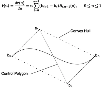
* The convex hull property states that the entire curve is contained within the convex hull of the control points.

* The first derivative of a Bezier curve is represented by

dr(u) n-1

i(u) du n

n

(bi+l - bi)Bi,n-1(), O < u < 1.

i=0

b,.

Convex Hull

bo b

Control Polygon

,/

"b2

Figure 3-1: A Cubic Bezier Curve with Control Polygon

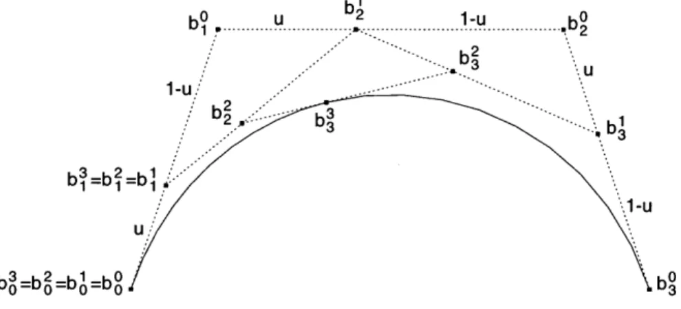
A B6zier curve can be evaluated at a specific parameter value uo and the curve can be split at that value using the deCasteljau algorithm, where [22, p.125]

(27)

is applied recursively to obtain the new control points. The algorithm is illustrated in Figure 3-2, and has the following properties:

* The values b9 are the original control points of the curve.

* The value of the curve at parameter value u₀ is bn.

* The curve can be represented as two curves, with control points (bn, bn,..., bn) and

(bn , bn - 1 bo )

* Since this is merely a change in the basis representation, the curve itself remains parametrically and geometrically unchanged.

b 32 b1=bI

bob=bo=bo

Figure 3-2: The deCasteljau Algorithm

B6zier Surfaces

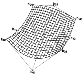
A tensor product surface is formed by moving a curve through space while allowing defor-mations in that curve. This can be thought of as allowing each control point bi to sweep a curve in space. If this surface is represented using Bernstein polynomials, a Bdzier surface is formed, with the following formula:

m n

R(u,v) = E EbijBi,m(u)Bj,n(v), i=0 j=

0< u, v <1.

Here, the set of lines drawn between consecutive control points bij is referred to as the

control net. An example of a bi-quadratic Bezier surface with its control net can be seen in

Figure 3-3. The following conditions apply:

*

The boundary isoparametric curves (u = 0, u = 1, v = 0 and v = 1) have the same

control points as the corresponding boundary points on the net.

* The corners of the surface coincide with the corner points of the net, and the deriva-tives in the u and v directions at the corners are tangent to the net.

* Bdzier surfaces exhibit the convex hull property.

(28)

Figure 3-3: A Bezier Surface with Control Net

Continuity Conditions

Bezier curves can represent complex curves by increasing the degree and thus the number of control points. Alternatively, complex curves can be represented using composite curves, which can be formed by joining several Bezier curves end to end. If this method is adopted,

the continuity between consecutive curves must be addressed.

One set of continuity conditions are the geometric continuity conditions, designated by

the letter G with an integer exponent. Position continuity, or Go continuity, requires the

endpoints of the two curves to coincide,

r(')(1) = r(2)(0).

The superscripts denote the first and second curves. Tangent continuity, or G1 continuity,

requires the tangents of the curves to be in the same direction, i(1)(1) = alt

i.(2) (0) = a2t

where t is the common unit tangent vector. G1 continuity is important in minimizing stress

concentrations and preventing flow separation.

Curvature continuity, or G2 continuity, requires the center of curvature to move contin-uously past the connection point,

i(2)-(0) = r2 l(1) + pi-f (1).

G2 continuity is important for aesthetic reasons and for preventing fluid flow separation.

More stringent continuity conditions are the parametric continuity conditions, where

Ck continuity requires the kth derivative of each curve to be equal at the joining point. In

other words,

dkr(l) (1) dkr(2_{) (0)}

(29)

The C1 and C2 continuity conditions for consecutive segments of a composite degree n Bezier curve can be stated as [44, p. 215]

hi;+ (bni - bni-1) = hi (bni+l - bni), and

bni-1 + h•+

hi

(bi-1

- bni-2) where, for the ith Bezier curve segment inclusively, hi = ti+1 - ti. See Figure 3-4.

(3.2) (3.3)

=

bi+i + (bni+l - bni+2) hi+1

with u values between knot values ti and ti+l

.hi+₁

b

'bn i+1

'bn i-1

Figure 3-4: Continuity Conditions

3.3 B-Spline Curves and Surfaces

The Bezier representation has two main disadvantages. First, the number of control points is directly related to the degree. Therefore, to increase the complexity of the shape of the curve by adding control points requires increasing the degree of the curve or satisfying the continuity conditions between consecutive segments of a composite curve. Second, changing any one control point affects the entire curve or surface, making design of specific sections very difficult. These disadvantages are remedied with the introduction of the B-spline representation.

A B-spline (basis-spline) curve is a piecewise polynomial curve meaning it is made up of polynomial curve segments. It is a spline curve with a different basis than the Bezier curves, although a Bezier curve is a special case of a B-spline curve. The B-spline representation has the advantage that the control points affect the curve only locally, and a B-spline of order k may have as many control points as required to describe the curve.

A B-spline curve is a series of polynomial segments of degree k - 1 joined together at

knots tk. A B-spline of order k (degree k - 1) with n + 1 control points has the equation

n

r(u) =

ZpiNi,k(u),

i=O

(30)

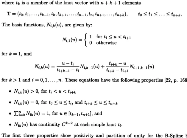
where tk is a member of the knot vector with n + k + 1 elements

T = (to, tl,. ., tk-1, tk, tk+1, ... , tn-1, tn, tn+l, ... 7 tn+k),

The basis functions, Ni,k(u), are given by:

1 NViI(u) = 0 to < tl • ... <- tn+k. for ti < u < ti+l otherwise for k = 1, and Ni,() = - ti ti+k - U

Nik)

i,k-l(u) + Ni+l,k-1(u)

ti+k-1 - i ti+k - ti+1l

for k > 1 and i = 0, 1,..., n. These equations have the following properties [22, p. 168]:

* Ni,k(U) > 0, for ti < U < ti+k

* Ni,k(u) = 0, for to < u

<

ti, and ti+k •< U < tn+k

*

;=oNik(u)

= 1, for u E [tk-l,tn+1], and

* Nik(U) has continuity Ck - 2 at each simple knot ti. The first three properties show positivity

functions.

Pr-3 .

and partition of unity for the B-Spline basis

...

Pr P r+1

Pr-1

Figure 3-5: A Cubic B-spline Curve Segment with Control Polygon

Local control means that a single segment of the B-spline curve is controlled only by the nearest n points, and that any control point affects the nearest n spans. In other words,

changing pi affects the curve in the parameter range ti < < ti+k and the curve at a point

u where tr < u < t,+l is determined completely by the control points Pr-(k-1), ... 1 Pr.

The convex hull property for B-splines applies locally, so that a span lies within the convex hull of the control points that affect it. This provides a tighter convex hull property than that of a Bezier curve, as can be seen in Figure 3-6.

(31)

Figure 3-6: Convex Hull Property for a Cubic B-Spline Curve

Increasing the multiplicity of a knot reduces the continuity of the curve at that knot. Specifically, the curve is (k-p- 1) times continuously differentiable at a knot with multiplic-ity p (< k), and thus has C(k- p - l) continuity. Therefore, the control polygon will coincide

with the curve at a knot of multiplicity k - 1, and a knot with multiplicity k indicates C- 1

continuity, or a discontinuous curve.

As you can see in Figure 3-5, the endpoints of the curve may not coincide with the control polygon. However, repeating the knots at the end k times will force the endpoints to coincide with the control polygon. Thus a knot vector described by

T

=

(to, tl,..., tk-1, tk, tk+1, ... ,tn-tn, tn+l ... ,tn+k) k equal knots n - k + 1 internal knots k equal knots

will have to = tl = ... = tk-1 and tn+1 = tn+2 = ... = tn+k and hence the first and last control points of the curve coincide with the endpoints of the curve.

From this discussion, it can be seen that a B6zier curve of order k (degree k - 1) is a

B-spline curve with no internal knots and the end knots repeated k times. The knot vector is thus

T = (to, tl,..., tk-1, tn+l, ..., tn+k)

k equal knots k equal knots

where n + k + 1 = 2k or n = k - 1.

A B-spline surface is a tensor product surface using a B-spline basis. This is represented mathematically as

m n

R(u, v) = Z Pij Ni,k(u)Nj,l(v). i=o j=o

(32)

Knot Insertion

A knot can be inserted into a B-spline curve without changing the geometry of the curve. The new curve is identical to the old one, with a new basis where

n

SpiNi,k

(u)

i=O

over T = [to, tl,... t, tl₁+l,...]

when a new knot t is inserted between insert the knot, and is represented as

n+1

becomes E NiM ,k(U)

i=0

over T = [to, t1,... ,tl,t, tl+l,...]

knots t1 and t1+l. The deBoor algorithm is used to

p = (1 -

i)p-

1

+

alp. 1 i > 1 -k+2 (3.4) where 1 ai 0 uo--ti tl+k--1 -ti i<l-k+1 l+1<i l-k+2<i<l

I - k + 2 < i < 1

To evaluate a B-spline curve at a specific parametric value or to split the curve at that value, the deBoor algorithm is used to repeatedly insert the same knot until the control polygon coincides with the curve at the parametric value uo, or in other words, until the

multiplicity of the knot at uo = k - 1. Then,

Pi = Pi

Pk-1 = r(uo).

A B-spline curve is C' continuous in the interior of a span. Inserting a knot does not change the curve, so it does not change the continuity. However, if any of the control points

are moved after knot insertion, the continuity at the knot will become Ck- p -1, where p is

the multiplicity of the knot. Figure 3-7 illustrates a single insertion of a knot at parameter value u0o, resulting in a knot with multiplicity of one.

1 0

Po=Po _{p =p}₄

(33)

The B-spline curve can be subdivided into Bezier segments by knot insertion at each internal knot until the multiplicity of each internal knot is the degree k. The above algorithm

is also known as Boehm's algorithm [4, 5].

Knot Removal

Knot removal is the reverse process of knot insertion. This thesis uses the knot removal algorithm developed by Tiller [42], in which a knot is removed if and only if it leaves the curve or surface geometrically and parametrically unchanged.

To demonstrate the process, this example uses a cubic B-spline curve r(u) given by control points (p0,... , p) and knot vector (to,... t10) where to = ... = t3 = 0, t4 = t5 =

t6 = 1 and t7 = ... =

tio

= 2 as shown in Figure 3-8. As the basis functions only guarantee

Co continuity at u = 1, the first derivative may or may not be continuous there. Using the

C1 continuity condition (3.2), the first derivative will be continuous if and only if

(t7 - t4)(P3 - p0) =

(t

6 - W3)).3

(P

-Since t₄= t6 = u, 0 U-t 3 o t7 - U 0 p3 = 4 P2-t7 -t3 t7 - t3 Since pO = pi and pO = p, P3 = aP₃ T (1 - a3)pl a3 = U - t

_{t7 - t3}

(3.5)

Note that (3.5) is the same as the deBoor algorithm equation (3.4) for inserting a new knot

at u = 1, although the points and knots are numbered differently in this example.

A similar reasoning yields that fact that a knot u = 1 can be removed a second time if

and only if the second derivative is continuous, yielding

P2 = a2P2

+ (1

- a) 2

p = a3P

+

(1 - a3 )p2

u - ti

ai = i i = 2, 3 (3.6)

ti+p+2 - ti

and a knot u = 1 can be removed a third time if and only if the third derivative is continuous such that 2 3 pi = al + (1 - al)P

p

2= a2P

(1

2

p2 = a3P + (1 - as)p 3 u - ti ai = i = 1,2,3. (3.7) ti+p+3 - ti

Note that there are no unknowns in equation (3.5), one unknown, p2, in equation (3.6) and

two unknowns, p3 and p3, in equation (3.7).

For the knot removal process, first the right hand side of equation (3.5) is computed and compared to p0. If they are equal within a given tolerance, the knot and pg are removed.

(34)

If the first knot removal is successful, equations (3.6) are solved for p2 and compared: 2 P P-(1-a2)p2 P2 S2 2 P1 - a3P2

P2

₁ - a3

If the two values for p2 are the same, then the knot and control points pi and pi are removed and control point p2 is inserted.

If the second knot removal is successful, the third step is to solve the first and third equations of (3.7) for 3 p -

(1

- az)po Pi

-2

3

3 P -a3P3 1 -_a3

The two values are then substituted into the second equation of (3.7). If the result is within tolerance of p , then the knot is removed and control points p2, p2 and p2 are replaced by

pi and p .

1

2

2 P3

P2

P3

p

1=p2

p1=p1- 1p 0O1 2 P5=P4=P3 O i=2 3 0 1 2=3 p =p =p₀=Po p6=p5=p4=p3 tO=t =t₂=t3 t4 =t5 =t6 t7=t8 =t9=tlo

Figure 3-8: Knot Removal

This can be generalized to apply to any number of removals of any particular knot. For

the nth removal, there will be a system of n equations with n - 1 unknowns. If n is even,

two values of the final unknown control point will be calculated and compared. If they are within tolerance, the knot removal is successful. If n is odd, all new control points are computed and the final two are substituted into the middle equation. If the result is within the tolerance, the knot removal is successful. If the nth removal is successful, n control

points will be replaced by n - 1 control points.

Knot removal from a surface is performed on the m + 1 rows or n + 1 columns of control points. However, the knot removal is successful only if the knot can be successfully removed from each row or column. Therefore, the result must be checked for each row or column before any control points are removed.

(35)

NURBS

The non-uniform rational B-spline (NURBS) curve is represented in a rational form

r(u)=

o

wibiNi,k(U)

E•=,o

WiNi,k(U)

where wi > 0 is a weighting factor and Ni,k(u) are defined over a non-uniform knot vector.

A NURBS surface patch can be represented as

R(u, v) -

%= 3=

(uv)

=

Ej=o

ij

Ni,k

(u)Nj,l

(v)

where wij > 0 is a weighting factor. A uniform knot vector is one where the knots are

evenly spaced. If the knots are not evenly spaced, the knot vector is non-uniform. Thus, any knot vector with repeated knots is non-uniform. The NURBS representation of curves and surfaces allows the exact representation of figures such as circles, conics, quadratics,

and surfaces of revolution with rational profiles such as torii. If wi = 1 for all i or wij = 1

for all i, j, this representation is the same as the integral non-uniform B-spline described

previously. In this thesis, all the B-splines used are integral, but the development could be extended to include NURBS.

(36)

(37)

Chapter 4 Review of Differential Geometry

Properties of Developable Surfaces

4.1 Introduction

This chapter discusses the properties of ruled and developable surfaces. The representations and properties discussed herein are taken from classic texts by Struik [41], Kreyszig [26], Faux and Pratt [11] and Spivak [40].

4.2 Ruled and Developable Surfaces

Ruled Surfaces

A ruled surface is a surface generated by the motion of a straight line (a generator or ruling) through space [41]. A curve that passes through all the rulings of the surface is called a

directrix. Any point on the surface can be expressed as

R(u, v) = a(u) + v,(u) (4.1)

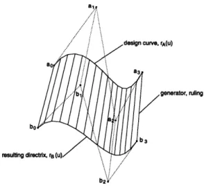
where a (u) is a directrix or base curve of the ruled surface and 3(u) is a unit vector which gives the direction of the ruling at each point on the directrix. Alternatively, the surface can be represented as a ruling joining corresponding points on two space curves. This is represented by

R(u, v) = (1 - v)rA(u) +vrB(U) 0 < U, v < 1 (4.2)

where rA(u) and rB(u) are directrices, as shown in Figure 4-1. The two representations are identical if

a(u) = rA(u) and

/3(u)

= rB(u) - rA(u). (4.3)

Throughout the thesis it is assumed that the constant u isoparametric lines correspond to the generators of the developable surface or, in other words, the straight line rulings are in the v direction.

(38)

ruling

direc

Figure 4-1: A Ruled Surface

Developable Surfaces - A Subset of Ruled Surfaces

Developable surfaces are a subset of ruled surfaces that have a constant tangent plane along

each generator. Since surface normals are orthogonal to the tangent plane and the tangent plane along a generator is constant, all normal vectors along a generator are parallel. This is shown in Figure 4-2.

normals

Figure 4-2: A Developable Surface with Tangent Plane along a Ruling

Given two points on a single generator that are selected at parameter values (uo, vl) and (uO, V2), the surface is developable if the tangent planes at these points coincide. The tangent planes are defined by the vectors R, and R,,. Using the representation of a ruled surface shown in (4.2), we obtain

drA (0) drB (u0)

Ru (no, j1)

= (1

-

vj)

_du

+ v,

_du drA(uo0) drB(uo0) Ru(U0O V2) = (1 - v2)

du

u +v2 du

du

(4.4)

(4.5)

(39)

Rv(uo, vi) = Rv(uo, v₂) = rB(u0) - rA(U0).

If the tangent planes at the two points coincide, the vectors R,(uo,vl), R,(uo,v2) and

rB(UO) - rA(UO) must be coplanar. Therefore, the triple product must equal zero:

IR,(uo,v

1 )

Ru(

0o,2)

(rB(U)

- rA(UO))I = 0.

(4.7)

Let Ru,(uo, vi) = Rau1 and Ru(uo,v2) = Ru2. Then

R1

x

R

2 1 2

-

RRu2] -

[R

R

₁ ₂-[R -

RYRX2lk

(4.8)

Expanding the first term of (4.ul8) by employing (4.4) and (4.5) yields

Expanding the first term of (4.8) by employing (4.4) and (4.5) yields

[(1 - V1)i

A

+ V liy1[(l - V2)W + V2i'B]

-[(1 - vl)i• + viir ][(1 - v 2)ZA + v 2iYB] -[(1 -Vl)i z4 + Vi V1][(1 -- V2)V'2( + v2r+B]

=

(1

-.vi)(1 - v2

)iAT

± 1(1 - v2)r rB + v2(1 - V1)iiz

+

±Vlv2YB

-[(1 - v)(1 - v2)Iy A

ij

Z + V1(1 - v2)i'Yi'~ + v2(1 - Vl)iAYB + Vlv2

rYBrZB

S(v₁- vlv₂- v2 + V1V2)i'iB + (v2 - V1V2 - v1 + VlV2)iAri

-

(v2

-

l)(i

-

iB)

Similarly,

RulRu2 - R1Ru2 = (v2 - vl)(iArB -

iiArB)

and

R - aRlt1 2 = (v2 - Vl) (ixR - ir B).

Therefore,

Rul x Ru2 = (V2 - Vl)(iA X rB)

and thus (4.7) can be reduced to

(rB(U) - rA(u)) X

i~A()

" iBB(u) = 0 (4.9)

for any u as long as vi 5 v2. Conversely, any surface that satisfies (4.9) must satisfy (4.7)

and, therefore, the tangent planes must be the same and the surface must be developable. Thus, a surface is developable if and only if (4.9) is satisfied. Substituting (4.3) into (4.9)

and using the fact that iA X rA = 0 yields the equivalent condition

Ax

x 3 =o.

(4.10)

Developable Surfaces - Envelopes of Families of Planes

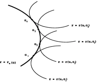
An alternative representation of a developable surface is as an envelope of a family of planes. The concept of an envelope will be described here for a family of curves, then extended to planes. First, we represent a curve as r(u, a) where u is the curve parameter and a is the family parameter. In other words, each curve in the family is r(u, an). There may be a curve re (a) that is tangent to each curve in the family, as shown in Figure 4-3. This curve (4.6)

(40)

would be the envelope of that family of curves [11].

= r(uax

r - r(u, )

K - X-UU'11

Figure 4-3: An Envelope of a Family of Curves

Similarly, a surface can be the envelope of a family of surfaces. Let a one-parameter family of surfaces be represented by G(x, a), where a is the family parameter, and assume that the surfaces are twice continuously differentiable. Also assume that consecutive surfaces intersect one another. The intersection is

G(x, a) = 0

G(x,a + h) = 0

where IhI is sufficiently small. This may also be represented by

G(x, a + h) - G(x, a)

=0.

(4.11)

The limit of (4.11) as h tends to zero is OG(x, a)/Oa = 0. The set of points represented by

G(x, a) = 0

OG(x, a) 0

Oa

is the characteristic of the surface. If the characteristics of all the possible surfaces in the family form a surface, that surface is called the envelope. If the envelope exists, then at every point of the characteristic of a surface in the family, the tangent planes of the surface and of the envelope coincide.

A characteristic point is determined by the intersection of the characteristic with another surface in the family. These points of intersection are determined by

0G(x, a)

G(x, a) = 0

G(xa)

0

-0 G(x, a + k) = 0.

where Jkl is sufficiently small. Using the Taylor series expansion

aG(x, a)

G(x, a + k)= G(x,a)+k

Oa k2 02G(x, a + Ok) +

2

, 0<0< 1, 2 802 r M 2

Analysis and design of developable surfaces for shipbuilding

Analysis and Design of Developable Surfaces for Shipbuilding

by

Julie Steele Chalfant

B.S., Mechanical Engineering

United States Naval Academy, 1988

Submitted to the Department of Ocean Engineering

and the Department of Mechanical Engineering

in partial fulfillment of the requirements for the degrees of

Master of Science in Naval Architecture and Marine Engineering

and

Master of Science in Mechanical Engineering

at the

MASSACHUSETTS INSTITUTE OF TECHNOLOGY

June 1997

@

Massachusetts Institute of Technology 1997. All rights reserved.

A uthor.

.. .

...

..

• ... ...

Department of Ocean Engineering

May 9, 1997

Certified by

...

...

Nicholas M. Patrikalakis

Professor of Ocean Engineering

Thesis Co-Supervisor

Certified by

. ...

...

...

Takashi Maekawa

L,ort~rer and Research Scientist

/

Thesis Co-Supervisor

C ertified by

...

.

...

... - ...

David C. Gossard

Professpr of Mechanical Engineering

rhesis Reader

Accepted by.

...

J. Kim

Vandiver

Chairman. DTa-atmental Committee on Graduate Students

DeDartment of Ocean Engineering

A

ccepted by ...

.. ...

Ain

Sonin

Chairman, Departmental Committee on Graduate Students

Department of Mechanical Engineering

JUL 1

5

1997

a"n

Analysis and Design of Developable Surfaces for Shipbuilding

by

Abstract

Acknowledgements

Contents

List of Figures

IKI

List of Tables

Chapter 1

Introduction

1.1

Background and Motivation

1.2

Research Objective

1.3

Thesis Organization

Chapter 2

_-N

_{= cos((7)lnllNI =}

_cos(7)